Force controlled haptic experiment with two different robots

(1)

Degree Course Systems

Engineering

Major: Infotronics

Diploma 2013

Franco Summermatter

Force Controlled Haptic

Experiment With Two Different

Robots

Professor

J o s e p h M o e r s c h e l l Expert

C h r is M a c n a b

Submission date of the report 2 7 . 0 9 . 2 0 1 3

(2)

(3)

(4)

Objectives

Realisation of a force controlled haptic experiment setup, which covers the system identification process for the used robots and the implementation of two different master slave operating scenarios with MATLAB/Simulink.

Methods | Experiences | Results

Two robots with different abilities are involved within this experiment, they build a haptic master-slave control system. Two operation scenarios were possible within this system were always one robot controls the other. Simulink acts as interface between the robots. Each scenario consists of a diagram for the simulation and a diagram for the real plant experiment.

To obtain the models used within the simulation diagrams, software tools were implemented which cover the different steps of the system identification procedure. Grey box modelling is used which permits to define precise linear or nonlinear model structures. The parameter for these models can be valued trough an estimation algorithm which is able to treat nonlinear plants.

The simulation and the real plant experiment can be actuated by the same artificial command signal, their output was compared and the models validated. The main purpose of the developed Simulink framework is to provide a tool to design more advanced controller setups within the experiment environment.

Force Controlled Haptic Experiment With

Two Different Robots

Graduate

Summermatter Franco

Bachelor’s Thesis

| 2 0 1 3 |

Degree course Systems Engineering Field of application Infotronics Supervising professor Dr Chris J.B. Macnab cmacnab@ucalgary.ca Partner

Schulich School of Engineering, University of Calgary

Alberta, Canada

First Robot: SensAble Phantom Omni Haptic Device. This root offers 3DOF force feedback and 6DOF position encoding.

Second Robot: Quanser 2DOF serial flexible joint robot. Each joint has one position encoder, one for the motor and one for the arm.

(5)

FORCE CONTROLLED HAPTIC EXPERIMENT

WITH TWO DIFFERENT ROBOTS

1 INTRODUCTION

The presented work is about a haptic experiment setup which includes two different types of robots. The first robot is a SensAble Phantom Omni, the second is a Quanser 2DOF1 robot with flexible joints (2DSFJ). Both robots are connected to the same PC and Simulink is used in external mode to control the robots. Two control scenarios are possible, as the master and the slave robot may switch their roles. The scenarios are defined as follow:

 Scenario 1: The Phantom Omni is the master, the 2DSFJ robot the slave.

 Scenario 2: The 2DSFJ robot is the master, the Phantom Omni the slave.

Each scenario has its own Simulink versions, one for the real plant experiment and one for simulation purposes.

The presented work covers beside the system description three major chapters: System identification, Scenario 1 and Scenario 2. The System identification chapter encloses all steps from data acquisition to model verification. Its goal is to find models, which repre-sent the robots in the simulation diagrams. The implemented software tools are explained alongside an example. The Scenario 1 and 2 chapter covers the designed Simulink dia-grams and their use for both scenarios. Simulation and real plant experiments use exactly the same controller, this makes is easy to simulate a controller design before implement-ing and testimplement-ing it on the real plant.

Within this work, only a basic controller is implemented which fulfills the task. It is intended as performance reference for more advanced controller designs. These controllers can be simulated and tested within the presented Simulink framework.

1.1 2 Channel Haptic Operation Principle

A haptic system for teleported robots consists of a master and a slave robot. In both sce-narios mentioned above, the operator applies a force on the master in order to achieve a proportional, desired force on the slave. The environmental force of the slave is feed back to the master. The operator feels the resistance of the slave against the movement on the master device dependant on obstacles or the environmental viscosity. This feedback force is proportional to the environmental force.

1

(8)

1.2 The Control Problem

The control problem involves the tracking of the master commands within two extreme sit-uations: Moving in free space and maintaining contact with a hard surface. The transition from one condition to the other should happen smoothly and without excessive force. The control scheme follows the force control principles presented in [1], were the command tracking is based on an augmented error which includes force and velocity signals.

No explicit torque or force sensors are installed on this system. This means that only the position measurements and the different robot abilities are used to obtain the force con-trol.

1.3 Tasks

The following tasks have been performed:

 Setting up the hardware.

 Implementation of Simulink diagrams which represent the hardware.

 Implementation of software tools to build models of the robots. These models are used to simulate the system.

 Implementation of Simulink diagrams for two operation scenarios. Each scenario has a simulation and a real plant representation.

 Controller design for both scenarios.

(9)

2 SYSTEM DESCRIPTION

This chapter contains a summary over the hardware used within the system. The robots are described here more in detail and their Simulink representations are presented. For the detailed hardware installation procedures, please refer to the corresponding operation manuals [2] and [3].

2.1 Overview

The system comprises the following main components:

 SensAble PHANTOM Omni

 PC with installed Software:

 MATLAB R2011a, Version 7.12.0.635

 Simulink with Quanser QUARC Toolbox, Version 2.2.1

 Q8 HIL2 PCI Board

 Q8 Terminal Board

 AMPAQ, Two Channel current amplifier

 Quanser 2DSFJ Robot

The following figure shows how these components are connected together. These con-nections don’t depend on the operation scenario and are always the same.

Figure 1: Deployment diagram of the system.

2 HIL Hardware-In-the-Loop AMPAQ Quanser 2DSFJ Phantom Omni Q8 Terminal Board Q8 HIL

(10)

2.2 Notations

To avoid confusion, the following definitions have been made in order to distinguish be-tween the Phantom Omni and the 2DSFJ robot:

 Phantom Omni: the two controlled arms are named Y-Axis for the first and Z-Axis for the second arm. The angular position uses the Greek letter .

 2DSFJ robot: the two controlled arms are named Stage1 and Stage2. The angular positions use the Greek letter .

The relation between master and salve robot arms is in every scenario:

 Stage1 ↔ Y-Axis.

 Stage2 ↔Z-Axis.

All MATLAB / Simulink files are named using the following prefixes for better structuration:

 A_... Refers to files, associated with the real plants (hardware operation).

 B_... Refers to files, associated with simulations (no hardware used).

 AB_... Refers to files, associated with the real plants OR simulations.

 C_... Refers to files, associated with system identification.

 D_... Refers to files, associated with verification.

To distinguish between the robots, the following midsection is used in filenames:

 …_2DSFJ_... Refers to the Quanser 2DSFJ robot.

 …_Omni_... Refers to the Phantom Omni haptic device. And to distinguish between the scenarios:

 …_Scen1_... Refers to the Scenario 1.

(11)

2.3 SensAble PHANTOM Omni Haptic Device

This haptic device (Figure 2) has 6-DOF position encoding which means 3-DOF for the three main axis (Cartesian or angles) and 3-DOF for the gimbal (angles). No force meas-urement sensors are installed on this device. The following subsections described the in-tegration of the hardware into usable Simulink blocks.

IMPORTANT NOTE: Before performing any powered operations, be sure the Phan-tom Omni has been calibrated!3

Figure 2: SensAble PHANTOM Omni [2], the force feedback abilities are 3-DOF for the mentioned main axis only.

2.3.1 Axis and sign convention

The Phantom block (Figure 3) from the QUARC library builds the core of the Omni Sim-ulink representation. This block can be parameterized for several types of haptic devices. It has the following sign definitions:

 X-axis: Left/Right movements, where Left is the positive direction.

 Y-axis: Up/Down movements, where Up is the positive direction.

 Z-axis: In/Out movements, where Out is the positive direction.

NOTE: The torque vector input has the same sign as the angles. That means i.e. a posi-tive torque input on the y-axis will move the arm upwards.

Figure 3: PHANTOM block, from the library QUARC/Targets

3

(12)

2.3.2 Horizontal operation mode

In order to have a more intuitive control experience and to avoid the gravity effect in the second scenario, the Omni has been put horizontally (Figure 4).

The sign definitions remain the same for the Y- and Z-Axis: CCW movements are read as positive.

Figure 4: Phantom Omni put horizontally. The neutral positions are indicated by black marks on the device casing.

Due to the internal construction of the Omni, a compensator block is necessary to com-pensate for the following effects while the device is put horizontally:

 Y-Axis: internal mechanical spring pulls the arm in positive direction.

 Z-Axis: arm movement drifts in one direction.

 X-Axis: must be blocked to keep the arm in a level position.

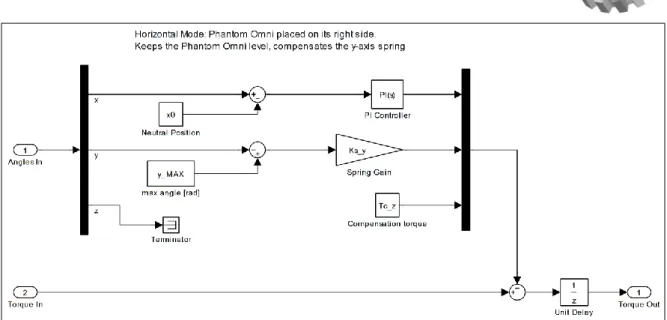
Figure 5 shows the internal layout of this compensator block. A PI-Controller on the X-Axis keeps the arms level, the mechanical spring is compensated by a fictitious spring on the Y-Axis and a constant torque is applied on the Z-Axis to overcome its drift.

Y-Axis Arm

Z-Axis Arm

w u

(13)

Figure 5: Compensator block layout, reduces the undesired effects when the Omni is put horizontally to a minimum.

2.3.3 Neutral position correction

Per default, the joint position angles which refer to the planes defined in Figure 4 have a range of:

 Y-Axis arm: 2 – 102 degree absolute referred to uw-plane.

 Z-Axis arm: 105 degree, referred to uv-plane. The limits of the Z-Axis are not abso-lute as they depend on the position of the Y-Axis arm.

NOTE: Due to the internal construction of the Omni, by moving the first arm around the Y-Axis, the measured position of the second arm is not affected. Actually, the device moves the Z-Axis as well in order to keep the position on the second arm.

The angle offset correction block (Figure 6) is used to convert the measured, pure positive range to a positive or negative range around a neutral position.

(14)

2.3.4 Velocity filter

To get the velocity measurement, the position signal coming from the Omni is derivated and low pass filtered. This happens inside the velocity filter block for both axes (Figure 7).

Figure 7: Velocity filter block, get the velocity out of position measurements.

2.3.5 Phantom Omni top level

All subsystem blocks mentioned in the previous subsections compose together the top level layout of the Phantom Omni block (Figure 8). This block is the base for all hardware depended Simulink diagrams. All parameters used are defined in the script phantomOmni_setup (code in Appendix 29). This script has to be executed to load these parameters into the workspace.

Figure 8: Phantom Omni block layout, takes a torque vector as input and gives a position and velocity measurement vector as output.

(15)

2.4 Quanser 2 DOF Serial Flexible Joint Robot (2DSFJ)

This robot (Figure 9) consists of two identical flexible joints. Each joint is equipped with a drive motor, a drive encoder and a joint encoder. The mechanical coupling between the driven part and the arm is realised with two compression springs. Each stage has its own harmonic drive and motor specifications. In the actual setup, the lightest springs are in-stalled on both stages.

Figure 9: Quanser 2DSFJ Robot [3]

2.4.1 Stages and sign convention:

The stages are defined in Figure 9, the shoulder joint is named Stage1 and the elbow joint Stage2.

 For both stages, CCW is the positive direction viewed from the Top.

NOTE: When the robot moves in positive direction (CCW) and hits an obstacle, then the applied force to this obstacle is positive. This means a CW deflection of the flexible joints is read as positive force.

NOTE: otherwise than stated in [3], the actual gear ratio of the harmonic drive #2 is 80:1 instead of 50:1.

2.4.2 Verification of the position sensors

The gear ratio of the flexible joint encoder Kgenc was set to 6.23 in order to achieve an

an-gular accuracy of less than 0.2º between the drive and the joint encoder on both joints. This accuracy was measured on ±80º absolute angle which means a max. relative angle error of ±0.25% within ±90% of the joint’s range.

2.4.3 Verification of the joint torsional stiffness K

s

The joint torsional stiffness Ks was verified to check which springs are installed and to

have a physically coherent reference for the system identification process. This could be done due the following relationship between the torque applied from the environment Tenv

and the angle deflection ∆θ:

Stage 1

Stage 2

(16)

( 1 )

Where Ks and ∆θ are defined as:

( 2 )

( 3 )

The index i references the corresponding joint. Kr stands for the installed spring rate, r is

the radius from the joint rotational axis to the hole where the spring is installed and d is the distance from the joint centerline to the hole. The angle deflection ( 3 ) is the difference be-tween the joint encoder 2 and the drive encoder 1 which complies with the signs defined in 2.4.1.

In order to verify the theoretical value for Ks found with ( 1 ), a known torque Tenv was

ap-plied to each joint and the angle deflection was measured with Simulink. An average value for Ks could be calculated. The method used was to hang on different weights at a given

distance to the flexible joint rotational axis.

The theoretical torsional joint stiffness for both joint with the lightest spring installed in the other hole is 3.926 [Nm/rad]. The measured average was 3.971 [Nm/rad] for the joint #1 and 3.891 [Nm/rad] for joint #2. The measurements are listed in Appendix 1.

Ks1 respective Ks2 are now verified and could be seen as fix parameters for the system

identification process.

2.4.4 Simulink interpretation

The robot is connected to Simulink over the PCI board Quanser Q8 HIL. The QUARC toolbox contains specific blocks to communicate with the Q8 board. Basically, this com-munication contains: reading the position encoders, reading the actual current and writing the commanded current to the current amplifier.

(17)

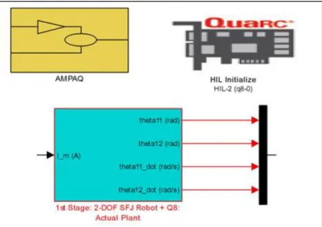
The general layout of one robot stage (Figure 10, lower block) is shown in Appendix 13. The basic layout was provided by an application example from Quanser it was adapted to fulfil the task. Additionally to the reading/writing operation, it consists of:

 a current limitation,

 a current correction to overcome the drift in one direction,

 a sign converter for the positive rotation direction,

 two second order low pass filters to obtain the angular velocities.

NOTE: In order to use the Simulink block described above, the block QUARC HIL initialize and AMPAQ must be present as well (Figure 10). These blocks contain the initialisation settings for the communication and the position limitation safety feature.

NOTE: The maximal continuous current after [3] is 0.94A for Stage1 and 1.2A for Stage2. However, these are max. values and it is recommended not to exceed 0.3 - 0.5A. As the robot movement will already be very quick.

All parameters necessary by the real plant related Simulink blocks are defined in the script robot_2DSFJ_setup (code in Appendix 28). Run this script to load these parameters in-to the workspace.

2.4.5 Safety feature

The 2DSFJ robot consists of two HAL sensors per stage. These sensors are located at the maximum and minimum physical position of the robot arm. If this safety is enabled (LIMIT_SWITCHES_ENABLE = 1) and one of the sensors is triggered, the execution of the running experiment will be stopped and an error message will be displayed.

The monitoring over these switches is included in the AMPAQ block provided from Quanser, see Appendix 14 for more details.

(18)

2.5 Signal Generator GUI

The signal generator GUI (Figure 11) is a key tool used for the experiment and simulation execution. It permits to simulate the master commands, dependant on the context this may be a position or a current.

All actuation signal parameter can be altered inside the GUI and a visual preview of these signals is offered. The user knows exactly which stage is enabled and how it will be actu-ated before the experiment/simulation execution. Additionally, the execution duration of the currently linked Simulink diagram can be altered directly in the GUI. The field Signal

Delay offers the option to delay the actuation signal. This is useful when actuating real

plant experiments in order to power up the robots first and start the actuation some time later. The simulation duration in the Simulink diagrams is set to a value: Simulation

Dura-tion + Signal Delay.

NOTE: The duration of the preview is the same as the simulation duration, the signal de-lay is not taken into account. If the simulation duration is set to 'inf' a maximum timespan of 100s is displayed.

Figure 11: The signal generator GUI provides a preview of the actuation signal before running the experiment. This saves time and inhibits surprised actuation signal patterns within the experiment.

The following actuation signals or their combination can be generated, the signals may be subject to user defined saturation:

 Step, with selectable amplitude.

 Amplitude sweep. (e.g. Figure 11, Stage 1 preview with saturation)

 Frequency sweep (chirp function). (e.g. Figure 11, Stage 2 preview with amplitude sweep)

(19)

The signal generator GUI is always connected to a main script which comprises the de-fault parameters and the name of the linked Simulink diagram. By executing the main script, the default parameters are loaded into the MATLAB workspace, the linked Simulink diagram and the signal generator GUI open.

Altering parameters within the signal generator GUI changes only their values inside the workspace. The Simulink diagram takes the current values from the workspace while exe-cuting.

NOTE: By running the main script again, all altered parameters are overwritten with their default values assigned in the main script.

The following figure shows the Simulink representation of the signal generator block:

Figure 12: Signal Generator block. The signal generator offers a wide variety of actuation signal patterns, from a simple step to amplitude modulated frequency sweeps.

The MATLAB code for the signal generator GUI was mainly auto-generated by MATLAB’s GUIDE4 tool. Therefore only the code for the opening function and the two main functions is attached in Appendix 30. The GUI concept is based on two functions, dependant on the field altered, one of these functions is called:

 updateFields: This function allows access to the different fields by enabling or disa-bling them if the corresponding checkbox is ticked. E.g. the amplitude sweep fre-quency setting may only be accessed if the checkbox Amplitude Sweep is ticked.

 updatePreview: This Function reads in all current values of the GUI and updates the values of the corresponding parameters in the workspace. It shows the calculated preview of the actuation signal. Every field related to signal settings calls this function if changed.

4

(20)

3 SYSTEM IDENTIFICATION

The purpose of the system identification is to find a model which can be used to simulate the systems behaviour for the controller design without the need of any hardware. As more accurate the model matches the real system, as more complex it will become. The model is always a trade-off between complexity and accuracy. Therefore simplifications are welcome but only if they affect the accuracy in an acceptable manner. This chapter explains the use of the implemented software tools to build models from data collection to model validation for each plant alongside an example.

The system identification process consists of the following steps:

 Experiment data acquisition.

 Model Structure definition.

 Parameter estimation.

 Model validation.

The system contains two independent plants, the Quanser 2DSFJ robot and the SensAble Phantom Omni haptic device. Each of them has its own characteristic and is treated inde-pendently with their own diagrams and parameter setups to obtain the models. However, the actuation signals are in both cases provided by the signal generator block.

There are several different procedures possible within the MATLAB System Identification Toolbox. Even though the model structure may be linear, the nonlinear grey box modelling was chosen because of the following advantages:

 Estimation according to parameters, (not location in state-space matrices).

 Individual parameters can be set to be fixed without touching the model structure.

 Flexible to adapt to additional parameters or another structure.

 Ready to treat nonlinearities.

However, the initial set up needs more effort because the model structure must be imple-mented in a function.

(21)

3.1 Quanser 2DSFJ Robot

This section covers the system identification steps for the 2DSFJ robot. The two stages are treated individually. However, all scripts and diagrams are common for both stages. One stage can always be disabled while the other is treated.

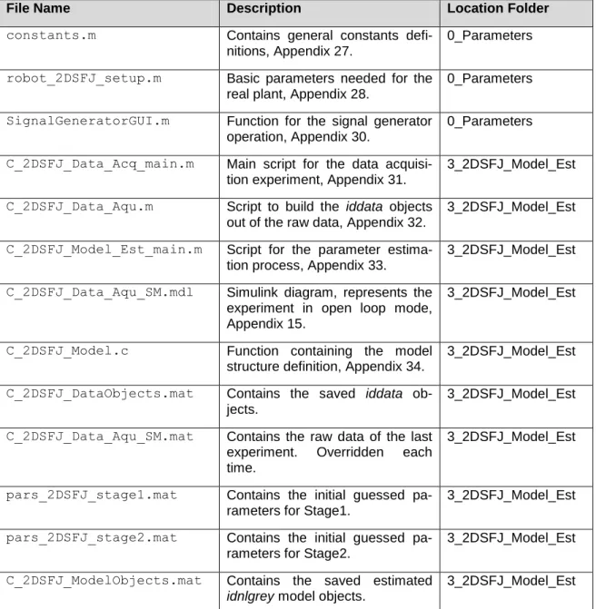
As the steps don’t differ from one stage to the other, only the procedure for Stage1 is mentioned here more in detail. The following table shows all MATLAB files associated with this section:

File Name Description Location Folder

constants.m Contains general constants defi-nitions, Appendix 27.

0_Parameters robot_2DSFJ_setup.m Basic parameters needed for the

real plant, Appendix 28.

0_Parameters SignalGeneratorGUI.m Function for the signal generator

operation, Appendix 30.

0_Parameters C_2DSFJ_Data_Acq_main.m Main script for the data

acquisi-tion experiment, Appendix 31.

3_2DSFJ_Model_Est C_2DSFJ_Data_Aqu.m Script to build the iddata objects

out of the raw data, Appendix 32.

3_2DSFJ_Model_Est C_2DSFJ_Model_Est_main.m Script for the parameter

estima-tion process, Appendix 33.

3_2DSFJ_Model_Est C_2DSFJ_Data_Aqu_SM.mdl Simulink diagram, represents the

experiment in open loop mode, Appendix 15.

3_2DSFJ_Model_Est

C_2DSFJ_Model.c Function containing the model structure definition, Appendix 34.

3_2DSFJ_Model_Est C_2DSFJ_DataObjects.mat Contains the saved iddata

ob-jects.

3_2DSFJ_Model_Est C_2DSFJ_Data_Aqu_SM.mat Contains the raw data of the last

experiment. Overridden each time.

3_2DSFJ_Model_Est

pars_2DSFJ_stage1.mat Contains the initial guessed pa-rameters for Stage1.

3_2DSFJ_Model_Est pars_2DSFJ_stage2.mat Contains the initial guessed

pa-rameters for Stage2.

3_2DSFJ_Model_Est C_2DSFJ_ModelObjects.mat Contains the saved estimated

idnlgrey model objects.

3_2DSFJ_Model_Est

(22)

3.1.1 Experiment Data Acquisition

1. Selection of the actuation signal

The quality of a model is highly dependent on the data used for the estimation process. Therefore a good experiment data set or sets are needed to perform successful parame-ter estimation. The selection of the actuation signal which guarantees as much useful in-formation as possible but without exceeding the plants physical limits is crucial. Several tests revealed, that high amplitude high frequency signals are best for the first estimation. This is especially important for plants with high dry friction.

To start a data acquisition experiment, open the MATLAB script C_2DSFJ_Data_Acq_main. On top of the script, the default parameter for the experi-ment can be altered.

NOTE: The parameter SIM_DELAY acts as transport delay for the actuation signal. The purpose of this delay is to avoid peak currents at the start of the experiment which may occur when the robot is powered and the actuation signal starts at the same time. Another reason is to start the experiment with initial states close to zero. This delay is removed au-tomatically form the captured data in the next step.

By running the script, the Simulink diagram C_2DSFJ_Data_Aqu_SM and the signal gen-erator GUI open. The Simulink diagram operates the 2DSFJ robot in open loop mode, the input signals amplitude unit is Ampere. Special care should be taken with amplitudes

above 0.1A for the first stage and 0.2A for the second stage, as the response may be very quick!

NOTE: By changing the simulation duration, a rebuild of the Simulink diagram is neces-sary. This can be done by selecting the open diagram and pressing Ctrl + B or selecting within Simulink the menu bar QUARC > Build.

2. Run the Experiment

With the actuation signal set, the experiment can be executed as usual within Simulink. The experiment data for both stages is logged into the file C_2DSFJ_Data_Aqu_SM.mat. Two demo data sets were collected for each stage. The actuation signal settings for these data sets can be found in Appendix 3.

NOTE: The experiment output file is saved in the current open folder in the file browser. In order to avoid error messages in the next step, the experiment should be run with the folder 3_2DSFJ_Model_Est open, where the execution file is located.

NOTE: Do not alter the values in the signal generator GUI between the experiment execu-tion and the data set build in the next step. The script C_2DSFJ_Data_Aqu uses the cur-rent values from the workspace. By changing these values in the meantime, the infor-mation stored in the iddata objects will be false.

(23)

3. Analyse the Experiment Data

After the experiment, the script C_2DSFJ_Data_Aqu provides treatment and analysis of the captured raw data. On top of the script, the dataset name which will be stored within the iddata object cell can be defined.

By running this script, the iddata objects are created according to the experiment settings, this includes the following steps:

 Remove the simulation delay.

 Extract the raw data input and output values for the enabled stages

 Build the data sets: Assign names, units, etc.

 Add information about the experiment according to the actuation signal settings. This information is displayed on the MATLAB console.

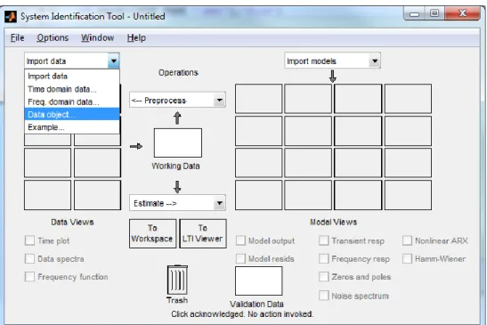
Next, the System Identification GUI opens (Figure 13). With this tool, the build iddata ob-jects can be imported and analysed easily.

Figure 13: System Identification GUI, to import a new data set, just select on the Import

(24)

Figure 14: Import Data Pop up Window, clicking on More shows information about the da-ta set.

Enter on the Import Data pop up window (Figure 14) the workspace variable name of a data set to be imported and by clicking on Import, the dataset appears on the left hand side of the System Identification GUI.

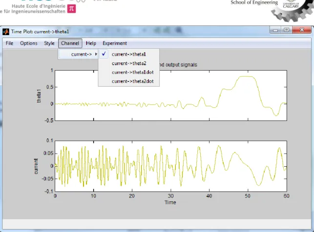
To analyze the imported data, check the box Time plot which opens a new window (Figure 15), displaying each input / output channel in the time domain.

(25)

Figure 15: Time plot, select under Channel every input/output combination. Experiment allows switching between the stages.

4. Store the Data Object

If the captured data seams correct and useful, the datasets must be stored manually in order to proceed with the model estimation process. The file data_2DSFJ.mat is meant to contain the saved iddata objects. To save a data set, rename it in the workspace and simply drag and drop it into the file.

NOTE: Data sets can also be exported to the workspace form the System Identification Tool GUI. This is useful if additional treatments like de-trending, resampling or another range etc. was applied within the GUI.

3.1.2 Definition of the Model Structure

With the experiment data ready for parameter estimation, it is now the time to define the model structure. As simpler the model structure as faster the parameter estimation pro-cess but on the cost of accuracy. On the other hand, if the structure becomes too complex with many parameters, it is more difficult to achieve good results. This is especially the case if many or all initial parameters are unknown.

The chosen linear model structure for the 2DSFJ robot results from its physical descrip-tion. The complete, simplified physical description is shown in Figure 16. The simplifica-tion consists of the hypothesis, that the drive #2 is installed on the center of gravity of the first stage. As each stage has its own independent position measurement, the system can be seen as decoupled and this hypothesis is reasonable. Please refer to Appendix 2 for the coefficient explanation and their corresponding initial values were applicable.

(26)

Figure 16: Complete physical schematic of the 2DSFJ robot [3].

Single Stage Model

After decoupling, the system can be reduced to two stages with identical differential equa-tions. Therefore, only the first stage is mentioned here more in detail. However, the pa-rameter values of each stage are different to comply with the real system.

Figure 17: Physical schematic of Stage1.

The schematic above gives the following system of motional differential equations for the two moving bodies:

̈ ̇

( 4 )

With the applied motor torque defined as:

(27)

State-Space representation

These two differential equations are second order with two independent variables, the two angular positions and . This SIMO5 model can be represented in state space form using the general state-space equations ( 6 ).

⃗̇ ⃗ ⃗⃗

⃗ ⃗ ⃗⃗ ( 6 ) The two second order differential equations ( 4 ) and can be transformed into 4 first order differential equations by defining the state variables as the two angular positions and an-gular velocities of the two bodies. The state, input and output vector is defined as follow:

⃗⃗⃗⃗⃗⃗ ̇ ̇ ( 7 )

⃗⃗⃗⃗⃗ ( 8 )

⃗⃗⃗⃗⃗ ⃗⃗⃗⃗⃗⃗ ( 9 )

On the actual plant of the 2DSFJ robot, the two positions of each joint are measured with incremental sensors; the corresponding velocity is derivated from the position. Therefore all four state variables can be measured on the actual plant. By defining the output vector equal to the state vector, the measured and simulated values can be compared easily. The system, input, output and feedforward matrices of the resulting state-space model for the first stage are:

[ ] ( 10 ) [ ] ( 11 ) [ ] ( 12 ) ( 13 )

The state-space matrices for the second stage are analog to them of the first stage.

5

(28)

Nonlinear Grey Box Model Structure

Grey box modelling in MATLAB necessities the implementation of a function containing the model structure related to the state-space representation. This means for a given time and given states as input, the calculation of the derivative states and the system output as result. These equations can be extracted from the state space representation above and are implemented as a state equation function and an output equation function in the file C_2DSFJ_model.c (Function code in Appendix 34).

The model structure function can be implemented with the MATLAB programing language or i.e. in C. The implementation in C was chosen here because of the faster program exe-cution as there are many function calls within the estimation process.

But these C functions need a Gateway function (same as main in normal C, see Appendix 34 line 55ff) which acts as interface between MATLAB and C type definitions. This Gate-way function was taken form a MATLAB tutorial and is not further explained in this docu-ment. The reader may find more information in the MATLAB documentation.

NOTE: MATLAB cannot use the C functions directly, these have to be compiled into C-MEX files. The MATLAB command mex ‘filename.c’ must be used for this purpose.

3.1.3 Parameter estimation

The model structure is defined, the grey-box model function implemented and compiled. Now, the estimation for the defined parameters can take place. According to the 2DSFJ model structure, there are six parameters to be estimated for each stage: Ktg, Ks, J1, B1, J2, and B2.

The prediction error estimation method pem is used to estimate the free parameters. There are several options available within this method (refer to the MATLAB documenta-tion). One of the most significant is the setting of the initial states which can be Zero or Estimate. Dependant on the data set used and even if the initial states were zero, the selection of Estimate can give much better results.

Open the script C_2DSFJ_Model_Est_main. Several settings can be made for the esti-mation process:

1. Basic settings:

- Select the stage to be estimated: i.e. EST_AXIS = 1 for stage 1. - Assign the dataset for the estimation and the verification process, here:

o estData = demo_st1 o verDat = demo2_st1

2. Advanced settings:

- Select the max. No. of iterations per data points (MAX_ITER). As higher the number as longer the process will take.

- Select the minimal and maximal value for each parameter (PARS_MIN, PARS_MAX). The estimation function will respect these constraints.

- Select the increment step in data points per iteration (ITER_POINTS) for the estimation loop. This value can be chosen e.g. dependent on the amplitude sweep period time.

(29)

Example: Amplitude sweep frequency 0.1Hz means zero crossing every 5s, with a sampling time of 0.05s, this results in 100 data points between zero crossings.

For one single estimation step for the entire data set, choose:

ITER_POINTS = NO_DATA_POINTS.

- Specify model structure function name, No. of parameters in the model struc-ture and model order (FUNC_NAME, PARS_NBR, ORDER).

Every parameter in the model structure can be set to be estimated or not. To specify a pa-rameter not to be estimated set the field Fixed to true.

Example: grey2DSFJ.Parameters(2).Fixed = true; Means, the second parameter will not be estimated and remain on its initial value.

By running the script, the estimation process is displayed in the console and the actual es-timation result is shown in a new figure window dependant on the settings for ITER_POINTS.

3.1.4 Model Verification

If the defined model structure and the corresponding estimated parameters represent well the real plant, can be verified using the method compare from the System Identification Toolbox. This method takes an iddata object as reference and compares the output of one ore more models with this reference data. It is important when ever possible to use different data sets for the estimation and the verification process to guarante the model corresponds to the dynamic of the plant and not to the trends of a single data set.

Figure 18 shows the plot from such a comparison for stage 1, three models were compared:

- modSt1Init, using initial parameters without estimation.

- modSt1DampOnly, only the two damping coeffitients B1 and B2 were estimated, all others remained on their initial value.

- modSt1All, all parameters were estimated.

For all models (were applicable) the iddata object st1DemoData was used for the estimation process.

(30)

Figure 18: Stage 1 model verification demo, verData object was st1DemoData2 In every of the 4 measured outputs (Figure 18), modSt1All has the best match. It can be observed that modSt1Init, were all parameters remained on their initial values does not reproduce the real plants behaviour very well. Even though, this model uses parameter values very close to the physical properties (provided by Quanser). The estimated param-eters of all models are listed in Appendix 4.

NOTE: As a linear model structure is used to match a real plant which always has certain nonlinearities, the estimated parameters are not to be meant as absolute physical proper-ties. The estimated values must be interpreted as best combination to simulate the dy-namic behavior of the plant. However, if a more accurate model in terms of physical prop-erties is desired, more parameters must be fixed. But this will certainly affect the model performance.

The model modSt2All shows a good representation of the actual plant, the linear model structure is therefore acceptable.

One demo model (st1DemoModel and st2DemoModel) for each stage was estimated and saved in the file C_2DSFJ_ModelObjects.mat. Their parameter values and verification plots can be found in Appendix 5 and Appendix 6.

The models were estimated with the iddata objects st1DemoData respective

st2DemoData. They were verified with the iddata objects st1DemoData2 and st2DemoData2. The fit compared to the velocity signals of the verification data is:

 Stage1: 65.21% for the motor position and 72.71% for the robot arm position.

(31)

3.2 SensAble Phantom Omni

In this section, the system identification steps for the SensAble Phantom Omni haptic de-vice are described. The basic procedure is the same as in section 0, therefore only the dif-ferences are mentioned here. The following table shows all MATLAB files associated with this section:

0_Parameters phantomOmni_setup.m Basic parameters needed for the

0_Parameters C_ Omni_Data_Acq_main.m Main script for data acquisition

experiment.

4_Omni_Model_Est C_ Omni_Data_Aqu.m Script to build the iddata objects

out of the raw data.

4_Omni_Model_Est C_ Omni_Model_Est_main.m Script for the parameter

estima-tion process, Appendix 35.

4_Omni_Model_Est C_ Omni_Data_Aqu_SM.mdl Simulink diagram, represents the

experiment in closed loop mode, Appendix 16.

4_Omni_Model_Est

C_Omni_model_2DOF_c.c Function containing the linear model structure, Appendix 36

4_Omni_Model_Est C_Omni_nl_model_2DOF_c.c Function containing the nonlinear

model structure, Appendix 37.

4_Omni_Model_Est C_ Omni_DataObjects.mat Contains the iddata objects 4_Omni_Model_Est C_ Omni_Data_Aqu_SM.mat Contains the raw data of the last

experiment. Overridden each time.

4_Omni_Model_Est

pars_ Omni_yAxis.mat Contains the initial guessed pa-rameters for the Y-Axis.

4_Omni_Model_Est pars_ Omni_zAxis.mat Contains the initial guessed

pa-rameter for the Z-Axis.

4_Omni_Model_Est C_2DSFJ_ModelObjects.mat Contains the estimated idnlgrey

model objects

4_Omni_Model_Est

(32)

3.2.1 Experiment Data Acquisition

Other than the 2DSFJ robot, the Omni experiment is in closed loop configuration. This means the actuation signal form the signal generator will be a reference position. A P-Controller with gain 1 is used to control the position. This configuration is necessary due to the high influence of the dry friction.

As the data acquisition scripts are basically the same as used in 3.1.1, their MATLAB code is not attached to this document.

To start a data acquisition experiment, open the MATLAB script C_Omni_Data_Acq_main. The procedure and settings are the same as in 3.1.1, except of the following:

 Closed loop configuration: Actuation signal from the signal generator is a position ref-erence in radian.

 P-Controller is present, gain values can be adjusted.

 Data acquisition script C_Omni_Data_Aqu contains an additional offset correction feature. The position measurement of the Omni is absolute. This means that the posi-tion at power up is not set to 0 as it was the case with the 2DSFJ robot. The posiposi-tion tracking starts at the position where the arms are hold manually. This is usually not exactly at the neutral position. This offset can be calculated from the raw data as the mean value from the position output within the transport delay phase. The first 5 data points are ignored to reject possible peak values:

36. % position offset correction, mean value from first data points: 37. offset1 = mean(output.signals.values(5:startPoint, 1)); 38. % input: motor torque

39. in1 = input.signals.values(startPoint:end,1) +offset1; 40. % output: Omni states; phi, phiDot

41. out1(:, 1) = output.signals.values(startPoint:end, 1) -offset1; 42. out1(:, 2) = output.signals.values(startPoint:end, 3);

Figure 19: C_Omni_Data_Aqu code segment to remove a possible offset.

However, if the data is de-trended, which may give better results, the removal of this offset has no effect.

The top level of the used Simulink experiment diagram can be found in Appendix 16. It uses the phantom Omni block described in 2.3.5.

NOTE: When running the experiment for the Z-Axis, a strong movement of the Y-axis can be observed. This is due to the internal design of the Omni. However, this movement has negligible influence on the captured position data of the Z-Axis. For the demo data sets collected, the Y-axis arm was hold at its initial position manually.

(33)

3.2.2 Definition of the Model Structure

The Phantom Omni underlies a strong dry friction influence. This leads to the conclusion, that a linear model will not be able to represent the dynamical behavior of the device very accurate.

As in 3.1.2, the idea is to treat the axes independently for the same reasons. Without a clear knowledge of the internal design of the Omni device, the following general model of a robot arm was used for each axis to describe the physical constrains:

Figure 20: Basic robot arm, physical model. Were:

Symbol Description Unit

Jm Motor moment of inertia Kg.m2

Ja Robot arm moment of inertia Kg.m2

Ba Gear-box damping coefficient Nm.s/rad

Ka Gear-box stiffness coefficient Nm/rad

Bm Motor friction damping coefficient Nm.s/rad

Tm Applied motor torque Nm

phi1 Motor position rad

phi2 Robot arm position rad

Table 3: Linear robot arm model, physical parameters.

Linear approach

This physical description yields to the following motional differential equations for the two Bodies:

̈ ̇ ̇

̇ ̈ ̇ ( 14 ) In order to obtain the state-space representation, the state, input and output vector is de-fined as follows:

(34)

⃗ ̇ ̇ ( 15 )

⃗⃗ ( 16 )

⃗ ̇ ( 17 )

And the resulting state-space representation for one axis is:

[ ] ( 18 ) ( 19 ) [ ] ( 20 ) ( 21 )

The structure mentioned above was implemented in the function C_Omni_model_2DOF.c for the grey box modelling process. This function represents the model in linear form with the first 5 first parameters listed in Table 3.

(35)

Nonlinear approach

To improve the model performance, a more advanced description for the friction must be used. As described in [4], the nonlinear friction torque on the motor shaft can be modelled as:

̇ ̇ ̇ ̇ ( 22 )

With

Symbol Description

Fv Viscous friction coefﬁcient.

Fc Coulomb friction coefﬁcient.

Fcs

Used to model the Strieback effect. α

β Used to get a smooth model without discontinuity at zero velocity, which is more suitable for simulation

Table 4: Nonlinear friction model, coefficients.

By introducing this friction torque Tf, the linear friction coefficient Bm can be replaced and

the motional differential equations turn into:

̈ ̇ ̇

̇ ̈ ̇ ( 23 )

The nonlinear derivative state equations are now:

⃗̇

[ ]

⃗ [ ] ⃗⃗ [ ] ( 24 )

The output equation ( 17 ) remains untouched.

This structure with 9 parameters was implemented in the function C_Omni_nl_model_2DOF_c.c. The estimation procedure for the nonlinear model struc-ture remains the same as for the linear model, only the parameter needs to be updated.

3.2.3 Parameter estimation

With the more complex, nonlinear model structure and the fact that the initial values are unknown, a more advanced estimation algorithm must be used to obtain usable results. Even if the model structure gives a good description of the real plant, without the correct parameter values the performance will be bad. Furthermore, wrong initial guessed param-eters lead the estimation process in the wrong direction, it will take a lot more time and no useful results can be expected. To overcome this problems, the used algorithm is to start with the linear model with only 5 parameters and a iddata object with captured values, were the nonlinear behavior is not so important. The estimated values from this linear

(36)

model can then be used as initial guess for the nonlinear estimation process were 9 pa-rameters can be estimated.

To perform the estimation process, open the script C_Omni_Model_Est_main.

Figure 21: Estimation process algorithm.

The figure above shows an example of a possible data set going from high lo low fre-quency over time. Assuming a sampling time of 0.05s, the dataset will contain 1200 data points. The estimation process takes now the following steps:

1. Linear model estimation using the first 200 data points only. These are within the high frequency area of the data set (red arrow).

2. Nonlinear model estimation, executed in a loop which takes with each iteration more data points into account (e.g. first iteration data points 1 – 100, second 1-200 etc.). Each iteration takes more data points into account (blue arrows) and takes the esti-mated parameters from the previous iteration as start parameters.

The data set should start with high amplitude high frequency movements as the dry fric-tion is not significant here. Within the data set, the frequency can then be lowered which yields to slower movements were the nonlinear friction must be taken into account.

NOTE: Decreasing the max. iteration steps (MAX_ITER) does not always mean the estima-tion process will be faster, the opposite may be true. This is the case if one data set part needs more iterations inside the pem function to achieve good results. If these results are inaccurate, the next iteration starts with wrong initial parameters which leads to a long es-timation process with no useful results.

As rule of thumb can be said, if one iteration within pem takes more than 5-10 sec, try to restart with different settings. To stop the execution press Ctrl +c in the command window.

(37)

3.2.4 Model Verification

The following figure shows the performance of the nonlinear model compared to the linear model if both were estimated with all data points of an iddata object. The estimated pa-rameter for these models can be found in Appendix 8. As the position depends on the ve-locity, it is treated as secondary information about the model quality. More important is the velocity behaviour of the model compare to the measured data.

Figure 22: Y-Axis model verification, velocity comparison with estimation data (upper plot) and verification data (lower plot).

It can be observed that the linear model greyOMNI gives not a bad representation (44.5-46.8% fit), even at the lower frequencies. However, at the lower frequencies the amplitude is too high and at the higher frequencies too low. The model dynamic is too limited to give a better representation. The nonlinear model greyOMNInl performs far better over the whole frequency range (69.8-71% fit).

One demo model (yAxisDemoModel and zAxisDemoModel) for each axis was estimated and saved in the file C_Omni_ModelObjects.mat. Their parameter values and verifica-tion plots can be found in Appendix 9 and Appendix 10.

The models were estimated with the iddata objects yAxisDemoData respective

zAxisDe-moData. They were verified with the iddata objects yAxisDemoData2 and zAxisDemoDa-ta2. The fit compared to the velocity signal of the verification data is:

 68.47% for the Y-Axis

(38)

4 SCENARIO 1: MASTER PHANTOM OMNI, SLAVE 2DSFJ

ROBOT

In the previous chapter, model structures of the real plant were defined, their parameters estimated and their performance verified. In this and the next chapter, these models are now used to implement simulation diagrams which represent the plants in the two scenar-ios. Each scenario contains one Simulink representation for the simulation and one for the real plant experiment.

4.1 Operation Description

In this first scenario, the Phantom Omni haptic device controls the 2DSFJ robot. The Y-Axis controls Stage1 and the Z-Y-Axis Stage2. Two major situations can be distinguished, the movement in free space and the contact with a hard surface.

As the Omni does not enclose a force measurement sensor, a fictitious spring is used to get a force measurement according to the position.

Movement in free space:

The operator moves the Omni in a desired direction, as farer away from the neutral posi-tion as more force must be applied due to a fictitious spring. The slave reacts to this commanded torque with a movement in the same direction at a speed proportional to the applied force. (Theoretically) no torque is applied from the environment to the slave, the operator feels no additional resistance to his commands.

Control mode: Torque → velocity, closed loop

In contact with a hard surface

When the slave touches a hard surface, its arm movement will be stopped. The torque applied from the robot to the environment can be measured by the joint deflection. This torque is feed back to the master with a proportional factor. The operator feels an addi-tional resistance on the master device.

(39)

The following table shows all MATLAB files associated with this section:

0_Parameters robot_2DSFJ_setup.m Basic parameters needed for the

0_Parameters phantomOmni_setup.m Basic parameters needed for the

0_Parameters A_Scen1_main.m Real plant setup, main script. 1_Scenario1 AB_Scen1_main.m Simulation OR real plant setup,

main script, Appendix 38.

1_Scenario1 B_Scen1_main.m Simulation setup, main script. 1_Scenario1 A_Scen1_RealPlant.mdl Simulink diagram, real plant 1_Scenario1 B_Scen1_Sim.mdl Simulink diagram, simulation. 1_Scenario1 D_Scen1_Exp_Analysis.m Script to analyse the captured

data, Appendix 39.

1_Scenario1 Scen1_createfigure.m Function containing figure

format-ting commands, used to plot simulation data.

1_Scenario1

C_2DSFJ_ModelObjects.mat Contains the models objects. 3_2DSFJ_Model_Est

Table 5: MATLAB files used within the first scenario.

4.2 Simulation

Figure 23 shows the basic layout used for both scenarios. The simulation and the real plant diagrams have exactly the same structure. A controller designed with the simulation setup can be included into the real plants setup simply by copy-paste. All input/output sig-nals to and from the controller block are the same.

Figure 23: Scenario 1 Simulation top level, the Simulink diagram structure for both scenar-ios consists of 3 main blocks: Master, Controller and Slave.

(40)

4.2.1 Master

The position movements on the master are simulated by the signal generator. The use of a model for the Omni has no influence to the simulation results and is therefore not nec-essary. However, the feedback loop is in place to comply with the real plant.

Figure 24: Scenario 1 Simulation Master block, two instances of the signal generator block are used to simulate the position movements of both axis. A gain block converts the posi-tion to a desired torque signals.

4.2.2 Slave

The slave blocks top level contains blocks for both robot stages (Appendix 17). Each stage (Figure 25) contains a nonlinear Grey-Box model block. The model used must be set in one of the scripts containing the simulation settings. The structure of the slave offers the possibility to simulate a hard surface with a saturation block, this block limits the movements of the model within a user defined range (ST1_WALL). A derivative filter must be used to get the velocity signal after the saturation.

NOTE: The wall contact saturation block should be used only on an informative base. The position within the model will not be affected by this block and the model output after re-turning from the wall contact may be inaccurate. So it may only be representative for the first wall contact.

Figure 25: Scenario 1 Simulation Slave, a saturation block permits the simulation of a con-tact with a hard surface.

(41)

4.2.3 Controller

The controller design follows the force control principle presented in [1] in a simpler PID-design. The basic idea is to have a 2 channel force control setup, which means to have a torque command from the master and a torque feedback from the slave. The controller should be able to control the slave in free space and while in contact with a hard surface without the need of changing the controller design or parameter values.

The torque error ( 25 ) is defined as the difference between the environmental torque Te

and the applied, desired human torque Td on the master:

( 25 )

The environment torque Te is defined as the torque applied from the robot to the

environ-ment:

( 26 )

Where Ks is the joint torsional stiffness. Ideally, in free space is equal to and the

en-vironmental torque becomes 0.

NOTE: To comply with the definitions in 2.4.1, a positive Te results if the robot arm moves

in CCW direction and hits a stiff surface. In this case will be greater than .

Control in free space

To control the robot in free space, a velocity penalty is added to the torque error which leads to the augmented error defined as:

̇ ( 27 )

With as a scale factor and ̇ as the motor speed of the 2DSFJ robot. If the controller can achieve s = 0 in free space were Te is 0, ( 27 ) will become to:

̇ ( 28 )

The slave velocity will be proportional to the desired torque.

Control in contact with hard surface

If Te is not 0, the commanded torque Tc is equal to Te plus the PI-controlled augmented

er-ror:

∫ ( 29 )

Which means Te will be equal to Tc if the controller can achieve s = 0. The commanded

torque depends on the difference between the actual position of the arm and the desired position of the motor multiplied with the joint torsional stiffness:

( 30 )

Which leads to the desired motor position:

(42)

By using the desired position, the actual position and the actual velocity of the motor, the commanded motor current will be:

̇ ( 32 )

The top level of the Simulink controller block is attached in Appendix 18. The equations above lead to the representation for one stage as shown in Appendix 19. This controller layout has 5 adjustable parameters for each stage. After trial and error, the values listed in the tables of Appendix 11 were found for the two stages.

4.2.4 Run the simulation

To run the simulation, open first the script B_Scen1_main (or AB_Scen1_main. and un-comment the simulation diagram)

After the loading section, the simulation setup section allows altering the basic settings like simulation duration, human torque gains as well as the model used within the simula-tion. The following sections contain the controller parameters, the default signal generator and feedback settings.

By executing the script, the Simulink diagram and the signal generator GUI open. The simulation diagram itself can then be executed as usual inside Simulink.

4.3 Real Plant

The real plant experiment (Figure 26) for the first scenario uses both robots. The experi-ment can be run in manual mode which means the master robot is actuated by a human operator or in simulated mode meaning the position of the master depends on a generat-ed position pattern. The fegenerat-edback loop permits the haptic control experience with scalable gain.

Figure 26: Scenario 1 Real Plant top level.

4.3.1 Master

The master block (Simulink diagram in Appendix 20) contains the Phantom Omni block described in 2.3.5 with some minor changes:

 The velocity signal isn’t used.

 The neutral position is maintained by fictitious springs (Figure 27). As farer away from the neutral position, as more force must be applied by the operator. The fictitious spring gain and the desired torque gain factor can be adjusted independently.

(43)

 In order to compare the behaviour of the controller to the simulation, the real plant of-fers on option to disable the manual actuation of the master device and use the signal generator instead (Figure 28).

NOTE: The master is meant to be held by the operator, especially with enabled feed-back. When using the real plant experiment in simulation mode, it is strongly recom-mended to disable the feedback loop.

 Feedback block (Figure 29), the gain of the feedback is adjustable and the feedback signal may be filtered. By filtering the feedback signal, the systems stability is im-proved when using higher feedback gains.

Figure 27: Position to torque converter block, calculates the spring torque and the desired torque out of the actual position of the device.

(44)

Figure 29: Feedback block, allows the feedback torque to be filtered.

4.3.2 Slave

The slave top level design is the same as in shown in Appendix 17, but each stage (Figure 30) contains now a 2DSFJ block described in 2.4.4.

Figure 30: Scenario 1 salve, implementation of Stage1. The environmental torque defined in 4.2.3 is measured inside this block, it is used for the controller and as feedback for the master.

4.3.3 Controller

The controller block used in the real plant experiment is identical with the one used in the simulation (see 4.2.3).

4.3.4 Run the Experiment

To run the experiment, open the script A_Scen1_main (or AB_Scen1_main. and un-comment the real plant diagram). A rebuild of the Simulink diagram may be necessary be-fore connecting to the target.

Executing this script opens the real plant Simulink diagram and if the manual mode is dis-abled, the signal generator GUI.

IMPORTANT NOTE: Before clicking on RUN in Simulink, be sure to put the Omni horizontally and hold the arms near to their neutral positions. This is also neces-sary when the manual mode is disabled, the Omni will be powered anyway!

(45)

4.4 Verification

To verify the performance of the designed controller as well as the behaviour of the model compared to the real plant, both, the simulation and the real plant Simulink diagrams can be actuated with the same generated input signal. To compare the output of this experi-ment, the script D_Scen1_Exp_Analysis can be used, this script plots the results in formatted form. The signal delay may be removed or not.

NOTE: The data collected from a real plant experiment were not saved directly into the workspace, they were stored in a realPlantExperimentName.mat file in the current open folder. This is due to the external running mode within Simulink. Each time the real plant experiment is run, this file is overwritten. The values from the simulation were direct-ly saved into the workspace.

To prevent overwriting the variables in the workspace before plotting, the analysis script should be run after each experiment or simulation. The simulation and experiment plots are displayed always in a new window. If the collected data needs to be available later, it must be saved manually.

4.4.1 Results: Simulation mode

Actuation signal:

The performance of the stages was verified using the following values for the generated position pattern:

Stage 1

Step response, amplitude 0.06 rad, torque gain 10Nm/rad, lambda 0.5, wall contact at 1 rad.

Stage 2

Step response, amplitude 0.08 rad, torque gain 10Nm/rad, lambda 0.5, wall contact at 1 rad.

The following plots show the simulation and the real plant experiment output for both stages:

(46)

Figure 31: Scenario 1 verification, Stage 1 simulation plot. Used model: st1DemoModel.

(47)

Figure 33: Scenario 1 verification, Stage 2 simulation plot. Used model: st2DemoModel

Force controlled haptic experiment with two different robots

Degree Course Systems

Engineering

Major: Infotronics

Diploma 2013

Franco Summermatter

Force Controlled Haptic

Experiment With Two Different

Robots

Objectives

Methods | Experiences | Results

Force Controlled Haptic Experiment With

Two Different Robots

Graduate

Bachelor’s Thesis

| 2 0 1 3 |

TABLE OF CONTENTS

FORCE CONTROLLED HAPTIC EXPERIMENT

WITH TWO DIFFERENT ROBOTS

1

INTRODUCTION

1.1

2 Channel Haptic Operation Principle

1.2

The Control Problem

1.3

Tasks

2

SYSTEM DESCRIPTION

2.1

Overview

2.2

Notations

2.3

SensAble PHANTOM Omni Haptic Device

2.3.1

Axis and sign convention

2.3.2

Horizontal operation mode

2.3.3

Neutral position correction

2.3.4

Velocity filter

2.3.5

Phantom Omni top level

2.4

Quanser 2 DOF Serial Flexible Joint Robot (2DSFJ)

2.4.1

Stages and sign convention:

2.4.2

Verification of the position sensors

2.4.3

Verification of the joint torsional stiffness K

Stage 1

Stage 2

2.4.4

Simulink interpretation

2.4.5

Safety feature

2.5

Signal Generator GUI

3

SYSTEM IDENTIFICATION

3.1

Quanser 2DSFJ Robot

3.1.1

Experiment Data Acquisition

3.1.2

Definition of the Model Structure

3.1.3

Parameter estimation

3.1.4

Model Verification

3.2

SensAble Phantom Omni

3.2.1

Experiment Data Acquisition

3.2.2

Definition of the Model Structure

3.2.3