HAL Id: hal-02985673
https://hal.archives-ouvertes.fr/hal-02985673
Submitted on 18 Nov 2020
HAL is a multi-disciplinary open access
archive for the deposit and dissemination of
sci-entific research documents, whether they are
pub-lished or not. The documents may come from
teaching and research institutions in France or
abroad, or from public or private research centers.
L’archive ouverte pluridisciplinaire HAL, est
destinée au dépôt et à la diffusion de documents
scientifiques de niveau recherche, publiés ou non,
émanant des établissements d’enseignement et de
recherche français ou étrangers, des laboratoires
publics ou privés.
The carbon balance of South America: a review of the
status, decadal trends and main determinants
M. Gloor, L. Gatti, R. Brienen, T. Feldpausch, O. Phillips, J. Miller, J.
Ometto, H. Rocha, T. Baker, B. de Jong, et al.
To cite this version:
M. Gloor, L. Gatti, R. Brienen, T. Feldpausch, O. Phillips, et al.. The carbon balance of South
America: a review of the status, decadal trends and main determinants. Biogeosciences, European
Geosciences Union, 2012, 9 (12), pp.5407-5430. �10.5194/bg-9-5407-2012�. �hal-02985673�
Biogeosciences, 9, 5407–5430, 2012 www.biogeosciences.net/9/5407/2012/ doi:10.5194/bg-9-5407-2012
© Author(s) 2012. CC Attribution 3.0 License.
Biogeosciences
The carbon balance of South America: a review of the status,
decadal trends and main determinants
M. Gloor1, L. Gatti2, R. Brienen1, T. R. Feldpausch1, O. L. Phillips1, J. Miller3, J. P. Ometto4, H. Rocha5, T. Baker1, B. de Jong18, R. A. Houghton7, Y. Malhi6, L. E. O. C. Arag˜ao8, J.-L. Guyot9, K. Zhao10, R. Jackson10, P. Peylin11, S. Sitch13, B. Poulter12, M. Lomas14, S. Zaehle15, C. Huntingford16, P. Levy16, and J. Lloyd1,17
1University of Leeds, School of Geography, Woodhouse Lane, LS9 2JT, Leeds, UK
2CNEN-IPEN-Lab., Quimica Atmosferica, Av. Prof. Lineu Prestes, 2242, Cidade Universitaria, Sao Paulo, Brazil 3NOAA/ESRL R/GMD1 325 Broadway, Boulder, CO 80305, USA
4Earth System Science Centre (CCST) National Institute for Space Research (INPE) Av. dos Astronautas, 1758 12227-010. S˜ao Jose dos Campos, Brazil
5Departamento de Ciˆencias Atmosf´ericas/IAG/Universidade de S˜ao Paulo, Rua do Mat˜ao, 1226 - Cidade Universit´aria – S˜ao Paulo, Brazil
6University of Oxford, Environmental Change Institute, School of Geography and the Environment, South Parks Road, Oxford OX1 3QY, UK
7Woods Hole Research Center, 149 Woods Hole Road, Falmouth, MA 02540-1644, USA
8School of Geography, University of Exeter, Amory Building (room 385), Rennes Drive, Devon, EX4 4RJ, UK 9IRD, CP 7091 Lago Sul, 71635-971 Bras´ılia DF, Brazil
10Nicholas School of the Environment, Duke University, Box 90338/rm 3311 French FSC-124 Science Drive, Durham, NC 27708-0338, USA
11CEA centre de Saclay, Orme des Merisiers, LSCE, Point courrier 129, 91191 Gif Sur Yvette, France 12Laboratoire des Sciences du Climat et l’Environnement (LSCE) Orme des Merisiers, Point courrier 129, 91191 Gif Sur Yvette, France
13College of Life and Environmental Sciences, University of Exeter, Rennes Drive, Exeter EX4 4RJ, UK 14Centre for Terrestrial Carbon Dynamics CTCD, University of Sheffield, Hicks Building, Hounsfield Road, Sheffield S3 7RH,UK
15Max-Planck-Institute for Biogeochemistry- Biogeochemical Systems Department, P.O. Box 10 01 64, D-07701 Jena, Germany
16Centre for Ecology and Hydrology, Bush Estate, Penicuik, Midlothian, EH26 0QB, UK
17School of Earth and Environmental Studies, James Cook University, Cairns, Queensland 4878, Australia 18El Colegio de la Frontera Sur (ECOSUR), Carr, Panamericana-Periferico Sur s/n, San Crist´obal de las Casas, 29290 Chiapas, M´exico
Correspondence to: M. Gloor (eugloor@googlemail.com)
Received: 30 November 2011 – Published in Biogeosciences Discuss.: 17 January 2012 Revised: 6 June 2012 – Accepted: 20 November 2012 – Published: 21 December 2012
Abstract. We summarise the contemporary carbon budget of
South America and relate it to its dominant controls: popu-lation and economic growth, changes in land use practices and a changing atmospheric environment and climate. Com-ponent flux estimate methods we consider sufficiently reli-able for this purpose encompass fossil fuel emission
invento-ries, biometric analysis of old-growth rainforests, estimation of carbon release associated with deforestation based on re-mote sensing and inventories, and agricultural export data. Alternative methods for the estimation of the continental-scale net land to atmosphere CO2flux, such as atmospheric transport inverse modelling and terrestrial biosphere model
5408 M. Gloor et al.: The carbon balance of South America
predictions, are, we find, hampered by the data paucity, and improved parameterisation and validation exercises are re-quired before reliable estimates can be obtained. From our analysis of available data, we suggest that South America was a net source to the atmosphere during the 1980s (∼ 0.3– 0.4 Pg C a−1) and close to neutral (∼ 0.1 Pg C a−1) in the 1990s. During the latter period, carbon uptake in old-growth forests nearly compensated for the carbon release associated with fossil fuel burning and deforestation.
Annual mean precipitation over tropical South America as inferred from Amazon River discharge shows a long-term upward trend. Although, over the last decade dry seasons have tended to be drier, with the years 2005 and 2010 in particular experiencing strong droughts. On the other hand, precipitation during the wet seasons also shows an increas-ing trend. Air temperatures have also increased slightly. Also with increases in atmospheric CO2concentrations, it is cur-rently unclear what effect these climate changes are having on the forest carbon balance of the region. Current indica-tions are that the forests of the Amazon Basin have acted as a substantial long-term carbon sink, but with the most recent measurements suggesting that this sink may be weakening. Economic development of the tropical regions of the conti-nent is advancing steadily, with exports of agricultural prod-ucts being an important driver and witnessing a strong upturn over the last decade.
1 Introduction
This review of the carbon balance of South America, with an emphasis on trends over the last few decades and their determinants, forms part of a catalogue of similar regional syntheses covering the globe as part of the RECCAP (RE-gional Carbon Cycle Assessment and Processes) effort. The scope of our analyses thus encompasses all methodologies as prescribed by RECCAP, including a “bottom-up” estimation of the net carbon balance through the assimilation of compo-nent flux measurements, simulations with Dynamic Global Vegetation Models (DGVMs) and atmospheric transport in-versions.
South America as a region has attracted the attention of global carbon cycle and climate researchers mainly because of the very large amount of organic carbon stored in the forests of the Amazon Basin. Occupying just less than half the area of the continent, these forests have been estimated to contain around 95–120 Pg C in living biomass and an addi-tional 160 Pg C in soils (Gibbs et al., 2007; Malhi et al., 2006; Saatchi et al., 2011; Baccini et al., 2012; Jobaggy and Jack-son, 2000; Table 1). Placing this in context, this ecosys-tem carbon stock (plants + soil) amounts to approximately half of the amount of carbon contained in the global atmo-sphere before the onset of the industrialisation in the 18th century. Thus, even if only a small fraction of this carbon
pool were to be released to the atmosphere over coming decades and/or centuries as a consequence of land use change or biome shifts associated with a hotter/drier climate, then the implications for the global carbon budget (and climate change itself) would be significant. On the other hand, be-cause of their vast area, high rates of productivity and rea-sonably long carbon residence times, these forests also have the potential to help moderate the global carbon problem through a growth stimulation in response to continually in-creasing [CO2], thereby mitigating the effects of some fossil fuel burning emissions (Lloyd and Farquhar, 1996; Phillips et al., 1998). Nevertheless, this effect must eventually satu-rate (Lloyd and Farquhar, 2008), and hence two main factors will likely dictate future changes in forest biomass. First and of primary importance is the way in which the current fast demographic and economic development (e.g. Soares-Filho et al., 2006) will impact on all ecosystems of the region. Sec-ond, changes in ecosystem carbon densities in response to changes in atmospheric gas composition and climate (e.g. Phillips et al., 2009), perhaps also in conjunction with biome boundary shifts (e.g. Marimon et al., 2006), may also be of considerable consequence.
The continuing development of the Amazon Basin is as-sociated directly with forest destruction mainly for agricul-tural use (e.g. DeFries et al., 2010). Changes brought about by altered climate and atmospheric composition on forests are subtler. Specifically, increases in carbon dioxide con-centration and/or changes in direct light may stimulate tree growth and in turn rainforest biomass gains (Lloyd and Far-quhar, 1996, 2008; Mercado et al., 2009), and there is strong evidence for such a process having occurred over the last few decades and to be still on-going (Phillips et al., 1998, 2009; Lewis et al., 2009). By contrast, a changing climate has, on the whole, been argued to be likely to have adverse effects on the tropical forests of the region. As for other parts of the globe, warming of the Earth’s surface is predicted to result in an increase in climate variation in South America (Held and Soden, 2006), and this includes a likely increased frequency and intensity of unusually dry periods. Such increased varia-tion, together with a general global warming, has the possi-bility to lead to forest decline through enhanced water stress. Drought induced forest loss may also be further amplified by fire (White et al., 1999; Cox et al., 2000; Poulter et al., 2010; Nepstad et al., 1999; Arag˜ao and Shimabukuro, 2010). Alto-gether, it is the interplay between the very large area covered by high carbon density and relatively undisturbed forests with the very fast economic and demographic development, and these interacting with a changing climate, which makes South America of particular interest for its role in the con-temporary carbon cycle and, in turn, to the climate of the planet over the decades to come.
This study aims to provide a state of the art assessment of the current day net carbon balance of South America through a review of carbon stocks and fluxes, their time trends, and their dominant controls. In doing this, we also describe how
M. Gloor et al.: The carbon balance of South America 5409
Table 1. Carbon stocks.
Inventory-based estimates
Woody biomass Soil organic carbon Reference
(Pg C) (Pg C)
Amazon (AD 2000) 121–126 164a Malhi et al. (2006) Tropical forest ∼95 Gibbs et al. (2007), Table 3 Extratropical forests ∼15b Gibbs et al. (2007), Table 3 Grass and shrubland ∼14c 102d
Agriculture ∼12c 76e
Remote sensing-based estimates Country Living woody biomassf Area
(Pg C) (106ha)
Tree cover threshold for forest definition (10 %/30 %) (10 %/30 %)
Brazil 54/61 442/596 Saatchi et al. (2011)
Peru 12/12 73/80 Saatchi et al. (2011)
Colombia 9/10 64/84 Saatchi et al. (2011)
Venezuela 7/7 47/61 Saatchi et al. (2011)
Bolivia 6/6 61/74 Saatchi et al. (2011)
Total Latin America 107/120 893/1209 Saatchi et al. (2011)
aAssuming the forest area from Malhi et al. of 5.76 × 10⁶km2, and a soil organic carbon content of 29.1 kg C m−2(Jobaggy and Jackson, 2000).
bAssuming forest biomass density of 200 t ha−1and forest areas of Paraguay, Chile and Argentina today based on the data in Table 4. cRough estimates based on vegetation type areas estimated by Eva et al. (2004) (see A.1) and biomass density of 30 Mg C ha−1for Grass and shrubland and agriculture.
dAssuming a soil carbon content of 23.0 kg m−2(Jobaggy and Jackson, 2000, their Table 3). eAssuming a soil carbon content of 17.7 kg m−2(value for crops of Jobaggy and Jackson, 2000). fBoth above- and belowground.
the carbon balance of South America has changed over recent decades and also provide an indication of what to expect in decades to come.
In order to quantify the continent’s net carbon balance, we have adopted an “atmospheric” perspective. This can most easily be envisioned as a consideration of all fluxes across an imaginary vertical wall all around the continent’s margin. Any carbon leaving the box enclosed by these walls (which is also imagined to have an infinite height) is a net carbon loss for South America (and a carbon source for the atmo-sphere), and vice versa. From this perspective, any internal transfers within the box – for example, the flow of detritus to rivers and/or its subsequent release as respired CO2– is “car-bon neutral” and thus does not need accounting. Similarly, al-though savanna fires may release substantial amounts of car-bon to the atmosphere each year (van der Werf et al., 2010), only a fraction of the continental savanna area burns in each year, and the unburnt areas (almost all of which will be re-covering from previous years’ fires) accumulating biomass (Santos et al., 2004). Thus, as long as the total area of savanna (of any other vegetation type) remains unchanged, such “in-ternal” fluxes can be ignored using our approach.
The paper is structured as follows. We start with a char-acterisation of main biomes, stocks, mean climate, climate trends, demography and economic development. We then present and discuss carbon fluxes associated with the dif-ferent processes and estimate them using complementary methods. The dominant processes, considered in a loose sense, fall into the categories of fossil fuel emissions, defor-estation, agriculture and trade, and forest biomass change. We then also discuss inferences from atmospheric green-house gas concentration data regarding the magnitude of car-bon sources and sinks through atmospheric transport inverse modelling and dynamic vegetation model estimates.
2 Main determinants of large-scale land surface changes and future energy consumption 2.1 Geography, population density, demography
Of the South American nations, Brazil is geographically by far the largest, occupying ∼ 49 % of the total area of 17.8 × 10⁶km2, followed by Argentina (16 %), Peru (7 %), Colombia (6 %) and Bolivia (6 %). Brazil is also the
5410 M. Gloor et al.: The carbon balance of South America
dominant economy of the continent, accounting for ∼ 50 % of the continent’s gross domestic product in 2009 and being the seventh largest in the world in terms of purchasing power parity (IMF, 2009).
The primary geographical pattern of the continent’s pop-ulation distribution (Fig. 1a) involves a band of very high density along the coastal arc stretching east and south from Venezuela, the Caribbean Sea and along the Pacific down to the South of Peru, and including the mega-cities Rio de Janeiro, S˜ao Paulo and Buenos Aires. This high population density along the coasts contrasts with the very low popula-tion density in the interior, especially within the still largely undeveloped Amazon Basin which covers an area of ∼ 8 mil-lion km2or nearly half the continent.
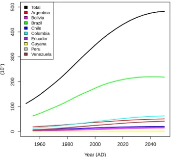
South America has witnessed very fast population growth, as well as increased urbanisation over the last 70 or so years (Fig. 2; Table 3). Rates of population growth remain substan-tial, but the continent-wide population is expected to stabilise at ca. 500 million inhabitants by around 2050 (Population Division of the Department of Economic and Social Affairs, UN, 2008).
In terms of “natural” ecosystem fluxes, one key region is the Amazon Basin, much of which remains covered by rela-tively undisturbed forest. Over half of the area of the Basin and its forest is located within Brazil (62 %), with the remain-ing 38 % spread across nine countries of which the largest landholders are Peru (7 %), Bolivia (6 %), Colombia (6 %), and Venezuela (6 %). As well as hosting the largest contigu-ous tropical forest area in the world, the Amazon Basin also abounds with a massive but still relatively unexploited min-eral and other natural resource wealth (e.g. Killeen, 2007a; Finer and Orta-Martinez, 2010). To date, however, develop-ment of the Basin has been mostly limited to a clearing of natural areas (of both forest and savanna) for cultivation and pasture. Improved access to global markets has played an im-portant role in this development, especially over recent years (e.g. Nepstad et al., 2006a; DeFries, 2010, Butler and Lau-rance, 2008; Finer and Orta-Martinez, 2010).
2.2 Biomes and their transformation over the last decades
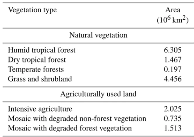
Based on the remote sensing estimates of Eva et al. (2004), the main vegetation and land cover types of South America include forest (45.2 % by area, ∼ 8.04 million km2), savanna and scrub lands (25.1 %) and agricultural land (24.1 %) (Ta-ble 2; Fig. 1b). These estimates refer to the time window of 1995–2000, with the remaining land covered by desert (At-acama, easternmost region of South America), water bodies and urban areas. Forest vegetation is predominantly located in the tropics, of which large parts are located within the Amazon Basin. Savanna type vegetation (the main belt to the south of the Amazon Basin generally being referred to as Cerrado in Brazil) originally stretched along a wide belt around the southern and eastern peripheries of the Amazon
Table 2. Vegetation cover of South America in 2000 ADa.
Vegetation type Area
(106km2) Natural vegetation
Humid tropical forest 6.305
Dry tropical forest 1.467
Temperate forests 0.197
Grass and shrubland 4.456
Agriculturally used land
Intensive agriculture 2.025 Mosaic with degraded non-forest vegetation 0.735 Mosaic with degraded forest vegetation 1.513
aEstimated by Eva et al. (2004) using remote sensing.
forest area (Eva et al., 2004), with coastal temperate forests to the east. Regions further south are used for agriculture, in-cluding sugar cane plantations in Sao Paulo state for the pur-pose of ethanol production and still further south for cattle grazing (southeastern Brazil and Argentina). Much of the lat-ter area was originally “Atlantic forest”, having been cleared many decades ago and with less than 1 % of the original for-est vegetation remaining (Dafonseca, 1985).
From a carbon cycle perspective, it is of interest that, un-like the temperate and boreal regions, tropical ecosystems have not been “reset” by glaciations (Birks and Birks, 2004), and thus their soils have developed on the same substrate over very long periods (Quesada et al., 2011). As a consequence, for large parts of the Amazon soil plant-available phospho-rus pools are low (Quesada et al., 2010), and phosphophospho-rus is a limiting element for growth for most forests of the Amazon Basin (Quesada et al., 2012).
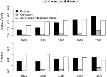
Although a large fraction of the Amazon is still covered by intact forest (∼ 82 % of the Brazilian legal Amazon by 2010, e.g. Fearnside, 2005; PRODES, 2010; Regalado, 2010), land use statistics for the Cerrado region within the Brazilian le-gal Amazon land shows that in 2006 approximately 60 % has been used for pasture and 15 % for cultivation, with the remainder constituting degraded or managed vegetation formation types (Fig. 3; AGROPECUARIA, Brazilian gov-ernment statistics). The fraction of cultivated land has ap-proximately doubled from 1975 to 2006, and so has its area (Fig. 3). This area change and timing matches approximately the time course and area of deforestation. Taking the area of Brazilian Cerrado (both within and outside the legal Ama-zon), this originally covered ca. 2 × 10¹²km2, but had de-creased to ca. 43 % of its original area by 2004 and will be entirely converted to agricultural use by around the year 2030 if annual conversion rates stay at their current level of 0.2 to 0.3 × 10¹²km2a−1(Machado et al., 2004).
The forests of the Amazon Basin have also been reduced in size at a fast pace, ∼ 0.46 % a−1since the early 1970s (e.g.
M. Gloor et al.: The carbon balance of South America 5411 a) b) Longitude Latitutde 80W 70W 60W 50W 40W 60S 50S 40S 30S 20S 10S 0 10N Evergreen Forest Deciduous Forest Seasonally flooded forest Temperate forest Agriculture Grass and Shrub Bare ground
Fig. 1. (a) Population density in South America in the year 2005 (CIESIN, 2005), and (b) land cover map of South America for 1995–2000
derived from remote sensing by Eva et al. (2004).
1960 1980 2000 2020 2040 0 100 200 300 400 500 Year (AD) (10 6 ) Total Argentina Bolivia Brazil Chile Colombia Ecuador Guyana Peru Venezuela
Fig. 2. Observed (until 2007) and predicted population growth for
South America by the United Nations (http://esa.un.org/unpd/wpp/ unpp/panel population.htm).
Fearnside, 2005), with one area of forest transformation cur-rently occurring along the so-called “Arc of Deforestation”
along the steadily northwards retreating southern periphery of the Amazon forest region. According to Fearnside (2005), by 2003 16.2 % of the originally forested portion of Brazil’s ∼5 × 10⁶km2of legal Amazon region had been deforested. Thus, compared to the Cerrado, a much larger percentage (83.8 %) of the forest area remains intact. This is in part due to the forest areas being more remote from economic centres, but also the soils of the forest–savanna transition zone are of-ten more fertile than those towards the centre of the Basin (Quesada et al., 2011) and, with rainfall still sufficient, sus-tain a high level of crop or pasture production. The moister
Cerrado regions also have the benefit of an aerial
environ-ment less conducive to crop disease pressures (Pivonia et al., 2004), especially in terms of temperature and moisture regimes that are markedly more seasonal than those of the core Amazon forest region. In addition, measures to protect Brazilian Cerrado have been far less reaching than measures to protect Brazilian rainforest (e.g. Fearnside, 2005).
Quantitative data on rates of deforestation for other coun-tries sharing the tropical forests, Peru, Colombia, Bolivia, Guyana, French Guiana, Suriname and Venezuela, are not so readily available. Nevertheless, remote sensing data cov-ering the period from 1984 to 1994 indicate a similar relative deforestation rate for Bolivia as for the Brazilian Amazon (Steininger et al., 2001; ∼ 0.4 % a−1). Deforestation rates for Peru have been lower, with rates between 0.1–0.28 % a−1
5412 M. Gloor et al.: The carbon balance of South America
1975 1980 1985 1995 2006
Land use Legal Amazon
Area (10 6km 2) 0.0 0.2 0.4 0.6 0.8 Pasture Cultivation
Agric. used / degraded forest
1975 1980 1985 1995 2006 Fr action 0.0 0.4 0.8 1975 1980 1985 1995 2006
Land use Legal Amazon
Area (10 6km 2) 0.0 0.2 0.4 0.6 0.8 Pasture Cultivation
Agric. used / degraded forest
1975 1980 1985 1995 2006 Fr action 0.0 0.4 0.8
Fig. 3. (a) Agriculturally used land by area in the legal Amazon, and (b) fraction of agriculturally used area by each of the three land use
practices (from IBGE, AGROPECUARIA 2006; http://www.ibge. gov.br/home/estatistica/economia/agropecuaria).
(Perz et al., 2005; Oliveira et al., 2007) and with a defor-estation rate of 0.1 % a−1applying to recent years (Oliveira et al., 2007). Although we have not found reliable data on deforestation for all South American countries with tropical forests, a pan tropical study for 1990–1997 based on a com-bination of 1 km2and higher resolution remote sensing prod-ucts (Achard et al., 2002) indicates similarly declining rates of land use change across the entire Basin as is now well doc-umented for Brazil. For both Brazil and Peru, the declining deforestation rates over the last few years (Regalado, 2010; Oliveira et al., 2007) have risen, at least in part, as a result of new government initiatives to try and help protect these forests (see also Nepstad et al., 2006b).
For the more densely populated sub-tropical and temper-ate zones to the south, land use change has since WWII been at even greater rates than for the tropics, specifically in Paraguay, Argentina and Chile. For these regions, many forest and woodland/scrub areas are now nearly entirely con-verted to agricultural use (Gasparri et al., 2008; Huang et al., 2009; Echeverria et al., 2006). The arboreal areas of the south have, however, always been of a relatively small mag-nitude compared to that of tropical South America (Table 4).
2.3 Climate and climate trends
Stretching from approximately 10◦N to 55◦S, South
Amer-ica’s weather and climate can be partitioned broadly into three zones characterised by different underlying atmo-spheric controls. The tropical zone (extending from north of the equator to ca. 22.5◦S) has its climate determined mostly by the westerly direction of the atmospheric circulation, the monsoonal circulation during austral summer, and the influ-ence of the Andes on lower tropospheric flow. The subtropi-cal region’s climate (ca. 22.5◦to 35◦S) is controlled by
semi-Table 3. Population growth and fossil fuel emissions, South
Amer-ica.
Year Population Fossil fuel emissions Year Population (AD) (106) (Pg C yr−1) (AD) (106) Censusesa Projectiona 1950 112 411 0.031 2015 412 665 1955 129 039 0.046 2020 430 212 1960 147 724 0.060 2025 445 428 1965 169 238 0.065 2030 458 052 1970 191 430 0.092 2035 468 111 1975 214 893 0.112 2040 475 482 1980 240 916 0.139 2045 480 436 1985 268 353 0.138 2050 482 850 1990 295 562 0.161 1995 321 621 0.192 2000 347 407 0.222 2005 371 658 0.242 2010 393 221
aFrom the Population Division of the Department of Economic and Social Affairs of the
United Nations Secretariat, World Population Prospects: The 2008 Revision, http://esa.un.org/unpd/wpp/unpp/panel population.htm.
permanent high pressure cells (centred around 30◦S), and finally for the mid-latitude southern part, by cyclones and anticyclones associated with the polar front in a generally westerly air flow (e.g. Fonseca de Albuquerque et al., 2009). Temperature trends over the last few decades estimated, for example, from the CRU climatology (Mitchell and Jones, 2005) reveal a warming trend for the Amazon Basin and Brazil, and constant temperatures or even a slight cool-ing of the continent to the south of Brazil and in the north-west of the continent (Colombia). Regarding precipitation, sufficiently long records for the purpose of robust trend anal-ysis exist, but unfortunately, with few exceptions, these are only available for outside the Amazon Basin (e.g. Haylock et al., 2006). The pattern revealed by these data is, how-ever, a positive trend in the region from approximately 20◦S down to Argentina and stretching from the eastern foothills of the Andes to the Atlantic coast. The second pattern is a decreasing trend in a stretch along the Pacific coast and up along the western flank of the Andes (CRU climatology; Mitchell and Jones, 2005; Haylock et al., 2006). The already mentioned increasing precipitation trend from approximately 20◦S southwards is mirrored by a strongly increasing trend of the La Plata River discharge into the Atlantic at Buenos Aires (e.g. Milly et al., 2005 and references therein). These positive trends are very likely the result of an increasing wa-ter vapour outflow from the Amazon Basin towards the south (Rao et al., 1996).
Because from a global carbon cycle perspective the Ama-zon Basin is by far the most significant South American re-gion, we further describe its climate in slightly greater de-tail as follows. The Basin’s climate is characterised by high annual mean precipitation (between ca. 1.5 and 3.5 m a−1) and relatively constant daily mean temperatures of 24◦ to
M. Gloor et al.: The carbon balance of South America 5413
Table 4. Estimates of forested area before the onset of intense deforestation in the 20th century.
Country Originally forested Year AD Region areaa Source area (106km2) (106km2)
Amazon and tropical South America
Bolivia 0.505 0.596 Killeen et al. (2007b)
Colombia (Amazonia and 0.631
Orinoquia) 0.130
Ecuador
Per´u 0.66 2005 0.647 Oliveira et al. (2007)
Venezuela (Amazonas) 0.178
Brazil, legal Amazon 4.0 1970 5.082 Fearnside (2005) Extra-tropical South America
Paraguay, Atlantic forest 0.624 1973 Huang et al. (2009)
Argentina 0.265 1900 Gasparri et al. (2008)
Chile (native forest area, 0.184 1990s CONAF (1999) i.e. not necessarily primary)
aFrom Perz et al. (2005).
26◦C (e.g. Nobre et al., 2009; Marengo and Nobre, 2009). The main element of the seasonal variation of the climate is the austral summer monsoon, which occurs during a period from roughly early October to the end of March. The rela-tively small Northern Hemisphere area has a seasonal cycle out of phase with the rest of the Basin by approximately 6 months. Associated with the (austral) summer monsoon is the rainy season followed by the dry season from approxi-mately April/May onwards. The dry season is not dry in the sense of the Northern Hemisphere mid-to-high latitudes but rather “less wet”, typically defined to include months with less than 100 mm of rainfall.
The main mode of inter-annual variation over recent decades has been associated with the El Ni˜no and La Ni˜na oscillation, collectively referred to as the El Ni˜no–Southern Oscillation (ENSO). El Ni˜no phases are associated with drier conditions in the north of the Basin and vice versa (Costa and Foley, 1999). Not all variation is controlled by ENSO (i.e. Pacific sea surface temperature (SST) variations). For exam-ple, cross-equatorial Atlantic sea surface temperature differ-ences influence the ITCZ (Intertropical Convergence Zone) location and thereby precipitation patterns as well (e.g. Yoon and Zeng, 2010). Also, on multi-decadal scales the domi-nance of Pacific and Atlantic influence vary (e.g. Yoon and Zeng, 2010; Espinoza et al., 2011).
Historically, Amazonian droughts have occurred fairly regularly, with a particularly intense episode in 1926 (Williams et al., 2005). Other unusually dry periods in the 20th century, mostly associated with El Ni˜no, occurred in 1935–1936, 1966–1967, 1979–1980, 1983 and 1992 (Marengo and Nobre, 2009). In more recent years, there have been strong droughts in parts of the Amazon in 1997/98, 2005 and 2010, with the latter two apparently related to At-lantic SST anomalies (Yoon and Zeng, 2010).
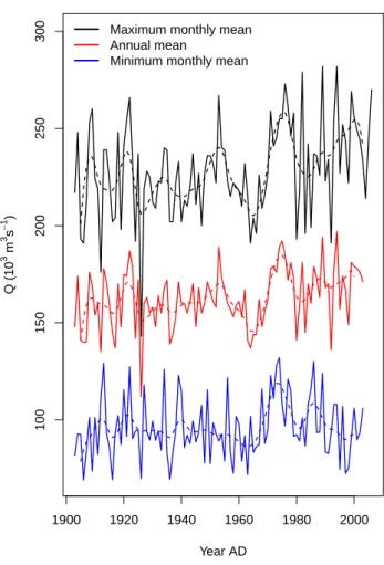
Similar to global land temperature trends, the Amazon region has warmed by approximately 0.5–0.6◦C over the last few decades (1960 to 2000, e.g. Victoria et al., 1998; Malhi and Wright, 2004). Published analyses of precipita-tion trends by various authors differ in the periods chosen, and climatologies or station data used (Espinoza et al., 2009). This is partially due to the sparsity of precipitation records in the Amazon already noted. Nevertheless, river discharge data should also provide a good diagnostic of hydrologi-cal cycle changes with the rate of discharge to the ocean providing a measure of the Basin-wide precipitation in ex-cess of plant requirements, and the following patterns emerge when analysing trends in Amazon river discharge at Obidos (Call`ede et al., 2004; Fig. 4), located approximately 800 km inland from the estuary of the Amazon River. At this point the River drains a basin of ∼ 4.7 × 10⁶km2, or roughly 77 % of the Amazon Basin proper. Although such data suffer from a shortcoming that the measured discharge is “blind” to whether water falling as precipitation has been recirculated via transpiration or not, as is shown in Fig. 4, the last ∼ 100 yr exhibit a substantial increasing trend (approximately 20 % change from 1900 to 2010), arguing for a similar trend in annual mean net precipitation. A second noteworthy feature which can be inferred from Fig. 4 is that wet seasons have become more pronounced and inter-annual variation has in-creased over the last decades.
2.4 Potential vegetation responses and feedbacks with climate
One widely cited hypothesis states that the anticipated in-crease in frequency and intensity of anomalously dry peri-ods in a warming climate may lead to a large reduction in forest vegetation and replacement by savanna, grasslands or even desert by 2100 (White et al., 1999; Cox et al., 2000;
5414 M. Gloor et al.: The carbon balance of South America 1900 1920 1940 1960 1980 2000 100 150 200 250 300 Year AD Q (10 3 m 3 s − 1 )
Maximum monthly mean Annual mean
Minimum monthly mean
Fig. 4. Maximum monthly (black), minimum monthly (blue), and
annual mean (red) river discharge at Obidos measured by Hydro-logical Service ANA, Brazil, http://www2.ana.gov.br/, and, where measurements are missing, estimated from upstream river gauge stations by Call`ede et al. (2004), based on data from the same data-source.
Oyama and Nobre, 2003). This hypothesis has, amongst oth-ers, been suggested by the first fully coupled climate–carbon cycle modelling results (Cox et al., 2000). However, more re-cent versions with a further evolved coupled climate–carbon cycle model from the same institution (Hadley Centre UK) do not show such a biome switch for the Amazon region (C. Jones, personal communication). Indeed, a data-oriented analysis by Malhi et al. (2009) which corrects for the fact that climate models are predicting a too dry contemporary climate finds a much lesser effect of a changing climate on tropical forest vegetation, and a climate ensembles approach shows the likelihood of forest “dieback” to be low (Poulter et al., 2010). Thus, although the possible risk of large-scale climate change induced forest “die-back” remains a concern and requires ongoing analysis and research, when correctly calibrated only a minority of climate models predict this pos-sibility at the current time.
Inventory data is especially of use for analysis of year-on-year features, and in some instances can give indications of what the Amazon forest response might be in a future cli-mate state (for instance, warm years might show features that become prominent in a continually warmer greenhouse gas-enriched world). The effect of atypical dry conditions on forest function have been examined by Phillips et al. (2009) based on tree growth and mortality data of a pan-tropical for-est census network. Looking at forfor-est dynamics following the “2005 drought” they found a small but significant increase in mortality compared to the long-term pre-2005 mean rate, suggesting a potential sensitivity of forest dynamics to more frequent or intense dry periods.
Besides climate alone, the 40 % increase in atmospheric CO2today over its pre-industrial concentration could in prin-ciple affect functioning of vegetation, specifically increasing photosynthetic rates, decreasing stomatal density and con-ductance, and thus leading to higher water use efficiency (e.g. Woodward, 1987; Lloyd and Farquhar, 1996, 2008). There are indications based on trends in the 13C :12C ra-tio of wood and leaf cellulose (the carbon isotopic rara-tio of wood is a strong function of stomatal conductance (e.g. O’Leary, 1988)) that there has indeed been down-regulation of stomatal conductance in parts of the Amazon forests (Hietz et al., 2005), although unambiguous attribution to mechanisms remains difficult (Seibt et al., 2008). Amazon River discharge and Basin-wide precipitation seem indeed, not having increased at the same rate, consistent with a trend in down-regulation of stomatal conductance (i.e. re-duced evapotranspiration; Gedney et al., 2006). Higher at-mospheric [CO2] may also favour the C3 photosynthetic pathway (mainly trees) over the C4 pathway (grasses, e.g. Ehleringer and Cerling, 2002). Several studies document for-est moving into savanna at the southern border of the Ama-zon forest-to-savanna transition Ama-zone with a speed on the or-der of 50 m a−1over the last 3000 yr, this being attributed to a shift in the ITCZ (Mayle et al., 2000). Significantly higher rates of “desavannisation” over the last decades are consis-tent with a [CO2] induced shift from C4towards C3 plants (e.g. Pessenda et al., 1998; Marimon et al., 2006).
3 Flux estimates
3.1 Fossil fuel and ethanol production and use
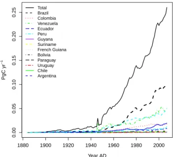
Currently, total fossil fuel emissions from South America are estimated to be 0.26 Pg C a−1, or approximately 3 % of the global total fossil fuel emissions (Boden et al., 2011; data available up to 2007). The increase since the 1950s has been approximately exponential, with an annual in-crease rate of about ∼ 8 % a−1 from 1950–1980 but falling back to 3 % a−1during the period from 1980–2008. (Figs. 6 and S1). Use of fossil fuels on a per person (pp) basis in 2005 was 0.65 Mg C pp−1a−1. This compared to a global
M. Gloor et al.: The carbon balance of South America 5415 1970 1980 1990 2000 2010 0 20 50 Soybean export (10 6 Mg yr − 1 ) Total Brazil Argentina Colombia Venezuela Peru 1970 1980 1990 2000 2010 0 5 15 Meat export (10 6 Mg yr − 1 ) 1970 1980 1990 2000 2010 0.00 0.03
Carbon export from plant cultivation
Year AD (PgCyr − 1 ) 1970 1980 1990 2000 2010 0 20 50 Soybean export (10 6 Mg yr − 1 ) Total Brazil Argentina Colombia Venezuela Peru 1970 1980 1990 2000 2010 0 5 15 Meat export (10 6 Mg yr − 1 ) 1970 1980 1990 2000 2010 0.00 0.03
Carbon export from plant cultivation
Year AD (PgCyr − 1 ) 1970 1980 1990 2000 2010 0 20 50 Soybean export (10 6 Mg yr − 1 ) Total Brazil Argentina Colombia Venezuela Peru 1970 1980 1990 2000 2010 0 5 15 Meat export (10 6 Mg yr − 1 ) 1970 1980 1990 2000 2010 0.00 0.03
Carbon export from plant cultivation
Year AD
(PgCyr
−
1 )
Fig. 5. Exports of agricultural products from five main South
American agricultural exporters according to FAO statistics (http: //faostat.fao.org).
average of 1.22 Mg C pp−1a−1 and is less than 15 % of more highly industrialised countries such as the USA (ca. 4.9 Mg C pp−1a−1).
One interesting aspect of fuel use in Brazil is that around 40 % of the total fuel used for motor vehicles and other com-bustion engines is ethanol (C2H6O) produced through the distillation of fermenting sugar cane (Macedo et al., 2008). Nevertheless, we do also note that biofuel usage is not in-cluded in the fossil fuel totals above. Compared to other crops, the ratio of renewable energy of ethanol/fossil fuel energy used to produce ethanol is high (8.3; Macedo et al., 2008). Ethanol utilization in Brazil in 2006 was 14.1 × 10⁶m3. To put this into perspective, the C flux to the atmosphere from burning ethanol in 2006 amounts to ∼5.8 Tg C a−1 (the density of ethanol which has a carbon content of 52 % is 0.789 Mg m−3), which is ∼ 5 % of the to-tal fossil fuel emissions from Brazil. However, because the carbon biomass used in ethanol production must have origi-nated from atmospheric CO2as recently assimilated by local sugar cane crops, these emissions do not contribute to the net carbon balance.
Ethanol production from sugar cane in Brazil goes back to the 1920s, originally developed as a means to utilize sugar cane overproduction. Currently, the main region where sugar cane is planted is in the southeast of Brazil (Sao Paulo State ∼ 66 %, Parana State ∼ 9 %, Minas Gerais State
1880 1900 1920 1940 1960 1980 2000 0.00 0.05 0.10 0.15 0.20 0.25 Year AD PgC yr − 1 Total Brazil Colombia Venezuela Ecuador Peru Guyana Suriname French Guiana Bolivia Paraguay Uruguay Chile Argentina
Fig. 6. Fossil fuel emissions estimated based on national energy
statistics (Marland et al., 2008).
∼9 %; UNICA, 2011). Both the production and export of ethanol have risen strongly over the last decade (produc-tion from 11.5 to 27.5 × 10⁶m−3and export from 0.2 × 10⁶ to 5.1 × 10⁶m3 in the years 2000 and 2009, respectively; UNICA Brazil, 2011). Although the area of ca. 7 × 10⁶ha−1 currently under sugarcane is not large compared to the ca. 200 × 106ha−1pasture (UNICA, 2011), there is strong con-cern and evidence that if expanding export markets are per-mitted to drive expansion of sugar cane plantation areas, then the deforestation frontier will move further north (e.g. De-Fries et al., 2010; Figs. 3 and 5).
3.2 Deforestation
Historically, global deforestation carbon emissions have been based on a book-keeping approach as detailed by the pioneer-ing study of Houghton et al. (1983). The area change data associated with land-use-change–related carbon fluxes used in these studies have traditionally been from the Food and Agriculture Organization of the United Nations (FAO), with the data provided to FAO by countries’ governments (see, e.g. Houghton, 2003). More recently, independent land use change area estimates – particularly those caused by defor-estation – based on remote sensing data and various statis-tical scaling approaches have become available (PRODES, Brazilian government; see Morton et al., 2005; Hansen et al., 2008; Achard et al., 2002, 2004). One advantage of these latter estimates is that they are more easily verifiable than the FAO data. Based on rates of change, it is then possi-ble to estimate land-use-change–related fluxes based on spa-tially explicit forest biomass estimates, e.g. from the RAIN-FOR forest census network (e.g. Malhi et al., 2002; Phillips
5416 M. Gloor et al.: The carbon balance of South America
et al., 2009), fraction of biomass combusted, and estimates of lagged carbon release and uptake due to decomposition of dead organic carbon and recovery after deforestation, respec-tively (Houghton et al., 1983).
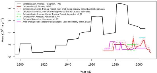
To progress along similar lines, in this study, we first com-pare the time course of forest area change (Fig. 7) based on FAO data (see e.g. Houghton, 2003), provided for this study by R. A. Houghton, with those coming from indepen-dent remote sensing-based estimates using sensors of vari-ous spatial resolutions. In some cases the remote sensing es-timates are based on a hierarchical approach using increas-ingly spatially resolving sensors to first identify “deforesta-tion hotspots” and then zoom in to hotspot areas using higher accuracy (Achard et al., 2002; Hansen et al., 2008). Figure 7 also includes estimates of changes in agricultural land use provided by the Brazilian government (Instituto Brasileiras de Geografia e Estatistica, Agropecuaria, 2006), which per-mits some test of consistency of the deforestation numbers. Although by no means a new insight, it is, however, clear that compared to the various independent remote sensing-based estimates (the numerical data are given in Table 5), the FAO area deforested numbers are substantially larger, even when considering that the different estimates are not for exactly the same regions. The independent remote sensing-based es-timates are quite consistent amongst each other and also con-sistent with the estimates of changes in agricultural land use in Brazil provided by the Brazilian government mentioned earlier on. We therefore base our further attempt to estimate carbon fluxes associated with forest clearing on the published remote sensing estimates of forest area change rates (i.e. in-dependently from the deforestation numbers of FAO).
The deforested area provides an upper bound on carbon release to the atmosphere if it is assumed that all forest car-bon (including roots and necromass) and soil carcar-bon fraction is lost after deforestation. Then the total carbon to be lost, Fld→at, is the product of the mean tree and soil organic mat-ter carbon per area multiplied by the deforested area, 1A, i.e.
Fld→at=rC:biom(Btrees+rsoil releaseCsoil)1A. (1)
Here, rC:biomis the carbon to biomass weight ratio, Btreesis tree biomass per area, rsoil releaseis the fraction of soil organic carbon released to the atmosphere, and Csoil is soil organic carbon content per area. By taking into account the time lags between the decomposition of dead organic material after de-forestation and similarly gradual replacement of the defor-ested area by a new (or potentially similar) vegetation type (Houghton et al., 1983), one can then estimate fluxes from differences in stocks. This provides a simple alternative to the accounting of individual fluxes within the continent which would involve, for example, a separation of deforestation-related emissions caused by fire from those which form part of a natural cycle (see Sect. 1). Below, we implement a sim-plified version of this so-called “book-keeping” procedure
with simple conceptualisation of the time lags in decompo-sition and time-course of establishment of a new vegetation cover. Our purpose is, in this relatively simple way, to bracket likely values of deforestation fluxes; our estimates reflect-ing the uncertainties of lags in carbon release and recovery whilst also taking full advantage of published deforested area estimates based on remote sensing. Specifically, we assume exponential decay of dead organic material left over from a deforestation event, i.e.
1C = −λrespC1t , (2)
where C is the carbon stock, 1C the annual release of car-bon to the atmosphere due to decomposing leftover debris, 1t a discrete time interval (one year), and λresp a decay constant. Establishment of new vegetation is assumed to ap-proach steady-state carbon content following
C(t) = Csteady(1 − e−λrgrwtht), (3)
where λrgrwthis the inverse of the time scale to reach a new steady state. The total flux to the atmosphere in year t caused by deforestation during year t and decomposition of dead or-ganic material remaining from deforestation events in previ-ous years is Fld→attot (t ) = t X tdef=−∞ Fld→at(t, tdef), (4)
where Fld→at(t, tdef)is the flux from land (“ld”) to the atmo-sphere (“at”) in year t due to deforestation in year tdefin the past. Similarly, the total flux from the atmosphere to land due to re-establishment of either forest or another vegetation type (we distinguish cultivation, secondary forest and pasture) is given by Fld→attot (t ) = t X tdef=−∞ X lu αluFat→ld(t, tdef), (5)
where Fat→ld(t, tdef)is carbon uptake in the wake of defor-estation in year tdef, and αluis the fraction of originally de-forested land being replaced by land use type “lu” each year (for details see Appendix). For αlu we use the values from Brazilian government statistics (AGROPECUARIA; Fig. 3), which due to lack of the same statistics for other coun-tries we assume to be similar. The model parameters are defined and values given in Table 6. Explicit expressions for Fat→ld(t, tdef)and Fat→ld(t, tdef)can be derived and are given in the Appendix. Following our goal to use deforesta-tion area estimates based on published, reproducible studies as much as possible, we have attempted an exhaustive search of the literature (Tables 5 and 7). Unfortunately, there are countries for which we did not succeed with our search. For three countries, Brazil, Argentina and Paraguay, we may re-construct reasonably well the land use change history from 1970 onwards. To proceed, we conceptually separate tropical from extratropical forest regions. To estimate tropical area
M. Gloor et al.: The carbon balance of South America 5417
Table 5a. Deforestation.
Year Area deforested Forest area Year Area deforested Forest area (AD) (103km2) (106km2) (AD) (103km2) (106km2)
Brazilian legal Amazon
Pre-1970 4.000a 1993 14.9 3.614 Pre-1978 3.931 1994 14.9 3.599 1978 20.4 3.890 1995 29.1 3.570 1979 20.4 3.869 1996 18.2 3.552 1980 20.4 3.849 1997 13.2 3.538 1981 20.4 3.829 1998 17.3 3.521 1982 20.4 3.809 1999 17.3 3.504 1983 20.4 3.788 2000 18.2 3.486 1984 20.4 3.767 2001 18.2 3.467 1985 20.4 3.747 2002 21.7 3.446 1986 20.4 3.727 2003 25.4 3.418 1987 20.4 3.706a 2004 27.8 3.399 2005 19.0 3.385 1988 21.1 3.684b 2006 14.3 3.373 1989 17.8 3.667 2007 11.7 3.360 1990 13.7 3.653 2008 12.9 3.352 1991 11.0 3.642 2009 7.5 3.346 1992 13.8 3.629 2010 6.5 3.340b
Latin America humid tropical forestc
1990 6.69 ± 0.57 1991 25.0 ± 1.4 1992 25.0 ± 1.4 1993 25.0 ± 1.4 1994 25.0 ± 1.4 1995 25.0 ± 1.4 1996 25.0 ± 1.4 1997 6.53 ± 0.56
Latin America humid tropical forestd
Brazil Americas sans Brazil
2000 0.72 % yr−1 2000 0.25 % yr−1 2001 0.72 % yr−1 2001 0.25 % yr−1 2002 0.72 % yr−1 2002 0.25 % yr−1 2003 0.72 % yr−1 2003 0.25 % yr−1 2004 0.72 % yr−1 2004 0.25 % yr−1 aFearnside (2005).
bPRODES, INPE, and Brazil, based on remote sensing. cAchard et al. (2002), based on remote sensing. dHansen et al. (2008), based on remote sensing.
deforestation over time, we scale the Brazilian tropical de-forestation numbers with a factor (100/79) as estimated by Hansen et al. (2008) for the 1990s (i.e. 1990–1999). For ex-tratropical South America we use the sum of the Argentina and Paraguay numbers. This will lead to a small underesti-mate because we neglect Chilean and Uruguayan deforesta-tion. For all of South America, αluis derived from Brazilian government statistics (AGROPECUARIA; Fig. 3), thus as-suming the same land use time history after deforestation for all of South America.
Simplifications and sources of uncertainty include the lim-itations due to the simple model formulation itself, the use of a spatial average wood density (supported by an analysis of RAINFOR data), scaling of deforestation area estimates, as-sumption of similar land use transition time patterns in South America as in the legal Amazon region, and uncertainty in the time scales for the decay of forest debris after deforesta-tion and for the re-establishment of a new vegetadeforesta-tion type af-ter deforestation. Error propagation yields a total uncertainty
5418 M. Gloor et al.: The carbon balance of South America
Table 5b. Deforestation.
Year Area deforested Forest area (AD) (103km2) (106km2) Andean Amazon Bolivian Amazon 1984–1987 15.5e 0.447e 1989–1994 24.7e 0.437e 1990–2000 15.06f 2000–2005 22.47f 2005/06 0.409f Peruvian Amazon 1985–1990 9.38h 1999–2005 3.88g 0.66g
Colombia no reliable data found (although see Sierra, 2000) Venezuela no reliable data found
Ecuador no reliable data found Extratropical South America Paraguay 1973 ∼0.624k 1970–1990 27.88ij 1990–2000 25.46j Argentina 1900 ∼0.026l 1970–1979 1.03k 1980–1989 1.38k 1990–1999 2.02k 2000–2005 2.08k
eSteininger et al. (2001), based on remote sensing (Landsat images, wall-to-wall). fKilleen et al. (2007b), based on remote sensing (Landsat images, wall-to-wall). gOliveira et al. (2005), based on remote sensing (Landsat images, wall-to-wall). hPerz et al. (2005).
iHuang et al. (2007), based on remote sensing.
jAssuming that Atlantic forest region is where most forest is being cleared. kAtlantic forest only.
lGasparri et al. (2008), based on remote sensing (Landsat images, wall-to-wall).
of the annual flux to the atmosphere due to deforestation of approximately ±25 % (see Appendix).
Our estimates indicate a net flux to the atmosphere of around 0.5 Pg C a−1due to deforestation and land use change in South America over the last two decades or so (Figs. 7 and 8). This has persisted over the last few years, despite the remarkable decrease in deforestation in the Brazilian Ama-zon, because of lagged fluxes caused by earlier deforesta-tion. Our estimate is smaller than the FAO estimate used in the recent study of Pan et al. (2011) for South America. The difference is smaller than expected based on the estimates of deforested areas alone, which by themselves differ strongly (Fig. 7). This is because the net flux to the atmosphere is the difference of release and regrowth and the regrowth esti-mate of Pan et al. (2011) is also much larger than ours. Thus,
the differences tend to compensate each other, and thus the global budget is not changed much.
3.3 Amazon forest censuses
Forest carbon storage and its trends have been monitored over the last few decades by keeping track of the diame-ter of all living trees within a permanent plot network. Two measurement strategies have been followed. One strategy (the CTFS (Center for Tropical Forest Science - Smithso-nian Institution) approach) samples a few plots of a rela-tively large size, 16–50 ha, of which there are currently three in tropical America (Chave et al., 2008). The other (the RAINFOR network; Phillips et al., 2009) currently samples 136 plots, mostly of 1 ha, covering the main axes of forest growth variation (El Ni˜no, soil fertility, dry season length; O. Phillips, personal communication). The censuses from the RAINFOR network have revealed a positive trend in above-ground biomass growth in the Amazon (dry matter, in units ha−1a−1)reported first by Phillips et al. (1998) and recently summarised in Phillips et al. (2009). These measurements do not include soil carbon trends, but this time series of inven-tory data is a significant step forward in understanding re-cent trajectories in the amount of carbon stored by Amazon forests. Given the labour and logistically-intensive require-ments associated with working in remote locations, then in-evitably the number of plots remains relatively few compared to what might be considered ideal, and, of course, that data is only available for the last few decades. Thus, there has been some concern expressed that the biomass accumulation (NEP) estimates are biased toward high estimates because rare large-scale disturbance events involving large biomass losses have not been captured (Fisher et al., 2008). Never-theless, an examination of this concern (Gloor et al., 2009) has concluded that, using a realistic (observed) disturbance severity and return time distribution, the results of a positive forest biomass gain trend based on the existing census net-work remain statistically significant and are unlikely to be an artefact. Other criticisms such as the uncertainty induced by using allometric equations for biomass estimation have been assessed and have also been demonstrated to have only minor impact on the regional sink estimates (Lewis et al., 2009). Results from a similar analysis based on the CTFS forest plots has confirmed a pan-tropical biomass increase trend, although of lesser magnitude (Chave et al., 2008). Here we do not use the results from this latter study, especially as only one plot is located in tropical South America.
We extrapolate the biomass changes reported by Phillips et al. (2009) to the tropical forests of all tropical South Amer-ica by first assuming a carbon content of wood of 50 % by dry-mass. Furthermore, following the compilation of Lewis et al. (2009; Supplement, p. 30) for estimating intact for-est area in the year 2000, we obtain a value of 703.3 ± 142 × 106ha (the value used is the mean of 630.5 × 10⁶ha from GLC 2000 (Global Land Cover Mapping for the Year
M. Gloor et al.: The carbon balance of South America 5419
Table 6. Parameters of book-keeping model to estimate deforestation carbon fluxes.
α =0.28 Fraction of dead biomass immediately released to the atmosphere after a deforestation event (Houghton et al., 1983).
αlu Fraction of originally deforested land being replaced
by land use type lu where lu can either be
cultivation, secondary forest, or pasture. We estimate these fractions from agricultural statistics for the legal Amazon (AGROPECUARIA, Brazil) and assume the same ratios throughout South America.
Coldgrowth forest=rC:Bio(1 + rblwgrd:abvgrd) Mean alive forest tree carbon content per area based ·220 (Mg C ha−1) on RAINFOR forest censuses.
Cforest soil=291 (Mg C ha−1) Oldgrowth forest soil carbon content
per area (Jobaggy and Jackson, 2000).
Cpasture=8 (Mg C ha−1) Carbon per area in vegetation of
pasture (Barbosa and Fearnside, 1996).
Ccultivation=50 (Mg C ha−1) Carbon per area in cultivation vegetation
(Barbosa and Fearnside, 1996).
Csecdry forest=0.8∗Coldgrowth forest Carbon per area in secondary forest vegetation (based on RAINFOR data).
rblwgrd:abgrd=0.2 Ratio of below- to aboveground tree biomass
(Malhi et al., 2010).
rsoil release=0.22 Fraction of soil C released to the atmosphere
when forest is converted to agriculture (Murty et al., 2002) (while according to Murty et al., 2002 the transition of forest to pasture does not lead to significant soil carbon loss).
rC:Bio=0.5 Ratio of carbon to rest of tree biomass by weight,
λoldgrowth forest=0.05...0.1 a−1 biomass decay rate of primeval forest debris
after deforestation (Achard et al., 2002).
λsecndry forest=0.05 a−1 Spin-up time scale for establishment of
secondary forest after deforestation (Schroth, 2002).
λcultiv=1 a−1 Spin-up time scale for establishment of cultivation
after deforestation.
λpasture=0.5 a−1 Spin-up time scale for establishment
of pasture after deforestation.
2000) – if dry and flooded tropical forest would be in-cluded, total tropical forest area would be 803 m × 106ha instead; 858 × 106ha from FRA CS (FAO Forest Resource Assessment, 2000); 780 × 106ha from FRA RS (FAO For-est Resource Assessment, 2000, remotely sensed values) and 544 × 106ha from WCMC (World Conservation Monitoring Centre). The first forest area estimate is based on the remote sensing instrument SPOT-VEGETATION (1 km spatial reso-lution); the second is “based primarily on available informa-tion provided and validated by nainforma-tional authorities” (Mayaux et al., 2005), the third estimate is based on “117 multi-date Landsat TM scenes covering approximately 10 % of tropi-cal forest” (Mayaux et al., 2005), with it not yet clear to us exactly what the last estimate is based on. From the four es-timates, the first three for all tropical forest are similar, while the fourth estimate is quite different.
We scale the tropical intact forest carbon sink in year a, f (a), originally in units of Mg DW ha−1a−1 (DW: Dry
Weight) from Phillips et al. (2009), Fig. 1, to total carbon flux F (Pg C a−1)using
F (a) = (1 + rBG:AGB)rC:DW(1 − λa
−1970
)A0f (a); (6)
rC:DW∼=0.5 is the ratio of carbon to dry weight of trees, A0 is the area of intact forest in 1970 before intense deforesta-tion started (∼ 817 × 106ha), λ ≈ 0.0046 (i.e. approximately 0.46 % forest area lost per year), estimated from deforesta-tion numbers based on PRODES from 1988 onwards and es-timates of Fearnside (2005) from 1970 to 1988 (Table 5). We also assume a belowground to aboveground tree biomass ra-tio of rBG:AGB=0.2 based on Malhi et al. (2009).
The resulting flux estimates are listed in Table 12 and shown in Fig. 9. The main features are a long-term (1980– 2004) carbon sink of 0.39 ± 0.26 Pg C a−1 in the mean (the uncertainty includes the contribution from area estimate vari-ation) with a reduction in the sink from 2005 onwards due to
5420 M. Gloor et al.: The carbon balance of South America 1900 1920 1940 1960 1980 2000 0 2 4 6 8 Year AD Area (10 6 ha yr − 1)
Deforstn Latin America, Houghton / FAO Deforstn Brazil, Prodes, INPE
Deforstn S America Tropical Forest, sum of all existg country based Landsat estimates Deforstn S America, sum of all existg country based Landsat estimates
Deforstn Latin America Humid Tropical Forest, Achard et al. 02 Deforstn Pan Amazon, Achard et al. 04
Deforstn S America, Hansen et al. 08
Area change cultiv+pasture+degrd&agric. used secondary forest, Brazil
Fig. 7. Comparison of various estimates of annually deforested area in South America, tropical South America, and Brazil, and annual change
in agriculturally used land in Brazil based on government statistics (AGROPECUARIA, same as in Fig. 3). The displayed estimates from top down are the following: (i) deforestation rate by area in South America according to FAO statistics (provided by R. Houghton in 2011), (ii) same but just for Brazil and estimated by INPE and Brazil based on Landsat images (PRODES, http://www.obt.inpe.br/prodes), (iii) same, based on PRODES and published studies of deforestation based on remote sensing (mainly Landsat) as listed in Table 4, (iv) same as (iii) but including in addition published remote sensing-based estimates for the rest of South America as listed in Table 4, (v) deforestation rate by area for Latin American humid tropical forests of Achard et al. (2002) based on remote sensing, (vi) same but for South America as estimated by Hansen et al. (2008), and (vii) total change in cultivated area per year due to agriculture in Brazil based on Brazilian government statistics (UNICA, http://www.unica.com.br/dadosCotacao/estatistica). 1970 1980 1990 2000 2010 −0.2 0.0 0.2 0.4 0.6 0.8 Year AD
Carbon flux to Atmosphere (PgC yr
−
1)
Net Flux to Atmosphere for λoldgrowth_forest=0.096
Net Flux to Atmosphere for λoldgrowth_forest=0.048
Net Flux to Atmosphere if carbon is released immediately and no regrowth Land carbon gain due to recovery to pasture
Land carbon gain due to recovery to cultivation Land carbon gain due to recovery to secondary forest
Fig. 8. Estimates of carbon released to the atmosphere from South America due to deforestation for two scenarios: (i) carbon is released
gradually and regrowth is taken into account using a simplified book-keeping model following Houghton (1983) as described in Sect. 3.2 and the Appendix, and (ii) all forest carbon after deforestation is released immediately to the atmosphere and there is no regrowth.
the on-going decomposition of dead trees arising as a conse-quence of unusually high mortality rates due to drought con-ditions in that year (Phillips et al., 2009). This carbon associ-ated with the drought-associassoci-ated mortality spike (∼ 1.2 Pg C) is modelled as not to have been released to the atmosphere immediately, but rather decaying exponentially in time and
thus reducing the Amazon Basin forest sink for several years to come.
M. Gloor et al.: The carbon balance of South America 5421
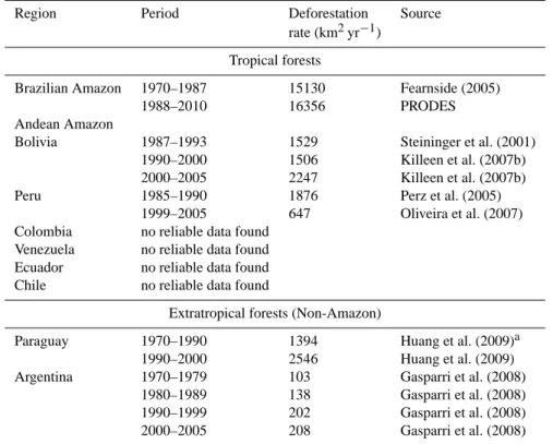
Table 7. Summary of published deforestation rates estimated mainly with remote sensing methods.
Region Period Deforestation Source
rate (km2yr−1) Tropical forests
Brazilian Amazon 1970–1987 15130 Fearnside (2005)
1988–2010 16356 PRODES
Andean Amazon
Bolivia 1987–1993 1529 Steininger et al. (2001) 1990–2000 1506 Killeen et al. (2007b) 2000–2005 2247 Killeen et al. (2007b)
Peru 1985–1990 1876 Perz et al. (2005)
1999–2005 647 Oliveira et al. (2007) Colombia no reliable data found
Venezuela no reliable data found Ecuador no reliable data found Chile no reliable data found
Extratropical forests (Non-Amazon)
Paraguay 1970–1990 1394 Huang et al. (2009)a 1990–2000 2546 Huang et al. (2009) Argentina 1970–1979 103 Gasparri et al. (2008)
1980–1989 138 Gasparri et al. (2008) 1990–1999 202 Gasparri et al. (2008) 2000–2005 208 Gasparri et al. (2008)
aAssuming that the Atlantic forest region is where most forest area is being cleared.
3.4 Inferences from atmospheric CO2 concentrations
and atmospheric transport
Depending on whether the land is a source or a sink, the effect of a carbon flux between land and the atmosphere is to either increase or deplete the CO2 concentration in the overlying air column. By keeping track of an air parcel’s path over a region of interest and by measuring the air col-umn CO2 increase/decrease along the air parcel path, it is thus possible, in principle, to estimate integrated net fluxes along the path. More generally, spatio-temporal concentra-tion patterns in the troposphere contain informaconcentra-tion on sur-face fluxes, which theoretically can be extracted by inverting and un-mixing the effect of atmospheric transport and disper-sion. This is done in practice using a 3-D atmospheric trans-port model in an inverse mode. For tropical South America, and the tropics generally, two obstacles do, however, make such an approach currently unreliable.
First and foremost, the troposphere around and inside the continent is highly under-sampled. Inverse methods can po-tentially provide information from remote observations in the tropical marine boundary layer or in the temperate lati-tudes. However, both transport modelling shortcomings and the inherent atmospheric dispersion that occurs over trans-port times of weeks from the tropical land surface to remote sites hamper that approach. As Stephens et al. (2007) showed for the tropics as a whole, tropical land flux estimates derived
1970 1980 1990 2000 2010 −1.0 −0.5 0.0 0.5 1.0 Year AD (PgC yr − 1 )
Carbon release from deforestation Fossil fuel burning emissions Intact tropical forest Carbon uptake
Fig. 9. Flux estimates from South America to the atmosphere (a
positive value indicates a flux to the atmosphere) due to deforesta-tion and a simplified book-keeping model, fossil fuel burning and carbon uptake by intact tropical forests.
from CO2observations at remote sites may reflect biases in-duced (propagated) by misfits in other regions of the globe.
Second, even with a single inversion model (in which transport is assumed to be perfectly known), the formal
5422 M. Gloor et al.: The carbon balance of South America 1980 1985 1990 1995 2000 2005 2010 −2 −1.5 −1 −0.5 0 0.5 1 1.5 2 2.5 3
Year AD
Land to Atm Flux (PgC yr
−1
)
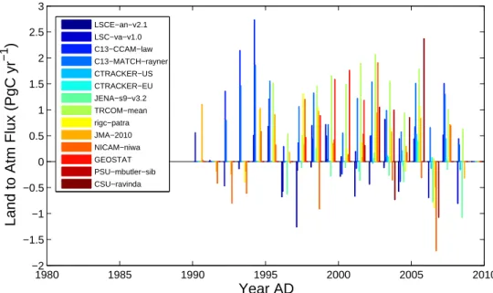
LSCE−an−v2.1 LSC−va−v1.0 C13−CCAM−law C13−MATCH−rayner CTRACKER−US CTRACKER−EU JENA−s9−v3.2 TRCOM−mean rigc−patra JMA−2010 NICAM−niwa GEOSTAT PSU−mbutler−sib CSU−ravindaFig. 10. Net carbon flux estimates from South American land to the atmosphere (i.e. a positive value is a flux to the atmosphere), estimated
based on atmospheric CO2concentration data and inverse modelling of atmospheric transport using a range of specific mathematical inversion
techniques prepared especially for RECCAP.
statistical uncertainties are very large, which reflect the loss of information during the transit of air-masses to the remote observation sites. The flux estimates based on classical atmo-spheric transport inversions in Fig. 10 reveal large scatter in the estimates among models, confirming our assessment of bias. Given that the estimates may largely reflect noise, we conclude their results not to be useful for the purposes of this study.
A new development with atmospheric sampling over South America is that recently joint efforts by IPEN (Sao Paulo, Brazil), NOAA-ESRL (Boulder, USA), University of Leeds (Leeds, UK) and University of Sao Paulo (USP) have led to regular vertical aircraft-based greenhouse gas sam-pling, with one/two stations (Santar´em, Manaus) operating since approximately the year 2000 and four aircraft sites from the end of 2009 onwards. These data should provide the necessary information to allow an atmospheric approach to be successfully applied for the quantification of the car-bon sources and sinks associated with both human activ-ity and natural biological processes, integrated across the Amazon Basin. An air parcel back-trajectory-based column-integration technique applied to the 10-yr record from San-tar´em reveals a moderate net carbon source of the land region upstream of Santar´em, and when fire related fluxes are sub-tracted on the basis of CO column enhancements, an approx-imately balanced land surface is found (Gatti et al., 2010). The region upstream of Santar´em covers only 10–20 % of the Basin and includes not only forests but also forest converted to agricultural use, as well as savanna and grasslands. It is thus quite likely that the balance of the entire Basin differs from this result.
3.5 Estimates from dynamic global vegetation models (DGVMs)
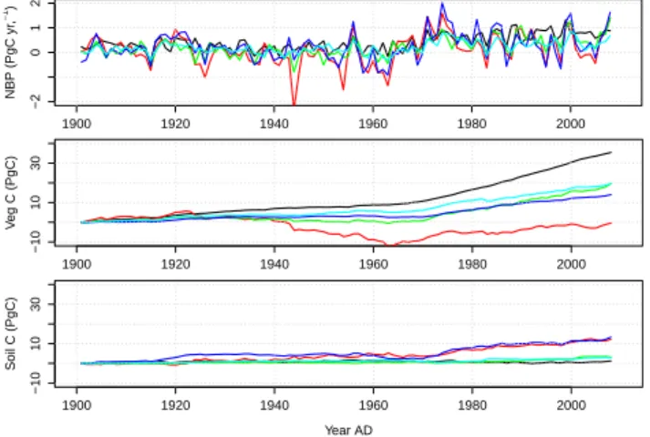
For this study modelling results from five DGVMs have been made available to us (TRENDY project, Sitch, personal com-munication). The models (DGVMs) were applied globally with common climate forcing and atmospheric [CO2] over the historical period 1901–2009 from a combination of ice core and NOAA annual resolution (1901–2009). A 6-hourly, 0.5◦global climate dataset was constructed based on merg-ing the observed monthly mean climatology from the Cli-mate Research Unit (CRU) and NCEP reanalysis. The mod-els were forced over the 1901–2009 period with changing [CO2], climate and land use according to the following sim-ulations: varying [CO2] only (S1), varying [CO2] and climate (S2), and varying [CO2], climate and land use and land cover change (S3, optional). Herein, we present results from sim-ulation S2. The various architectures and processes included by the models are summarised in Table 8 and the flux esti-mates in Table 11.
The main features of the simulation results of net biome productivity (NBP) (Fig. 11), where NBP is defined as
NB=NP−RH−F − QR, (7)
where NBis net biome productivity of land vegetation, RH heterotrophic respiration of land vegetation, F losses due to fire and QR carbon lost by riverine export, are as follows. Inter-annual and decadal variability of the model predictions are similar, nonetheless differences become apparent when fluxes are cumulated over time. With regards to cumulated changes in pool sizes, simulation results can be grouped into