A model-based evaluation of inversions of atmospheric transport, using annual mean mixing ratios, as a tool to monitor fluxes of nonreactive trace substances like CO 2 on a continental scale

HAL Id: hal-03115981

https://hal.archives-ouvertes.fr/hal-03115981

Submitted on 20 Jan 2021

HAL is a multi-disciplinary open access

archive for the deposit and dissemination of

sci-entific research documents, whether they are

pub-lished or not. The documents may come from

teaching and research institutions in France or

abroad, or from public or private research centers.

L’archive ouverte pluridisciplinaire HAL, est

destinée au dépôt et à la diffusion de documents

scientifiques de niveau recherche, publiés ou non,

émanant des établissements d’enseignement et de

recherche français ou étrangers, des laboratoires

publics ou privés.

A model-based evaluation of inversions of atmospheric

transport, using annual mean mixing ratios, as a tool to

monitor fluxes of nonreactive trace substances like CO 2

on a continental scale

Manuel Gloor, Song-Miao Fan, Stephen Pacala, Jorge Sarmiento, Michel

Ramonet

To cite this version:

Manuel Gloor, Song-Miao Fan, Stephen Pacala, Jorge Sarmiento, Michel Ramonet. A model-based

evaluation of inversions of atmospheric transport, using annual mean mixing ratios, as a tool to

monitor fluxes of nonreactive trace substances like CO 2 on a continental scale. Journal of

Geo-physical Research: Atmospheres, American GeoGeo-physical Union, 1999, 104 (D12), pp.14245-14260.

�10.1029/1999JD900132�. �hal-03115981�

JOURNAL OF GEOPHYSICAL RESEARCH, VOL. 104, NO. D12, PAGES 14,245-14,260, JUNE 27, 1999

A model-based evaluation of inversions of atmospheric

transport, using annual mean mixing ratios, as a tool

to monitor

fluxes of nonreactive

trace substances

like C02 on a continental scale

Manuel Gloor, Song-Miao Fan, Stephen Pacala, Jorge Sarmiento,

Carbon Modeling Consortium, Atmospheric and Oceanic Sciences Program and Department of Ecology and

Evolutionary Biology, Princeton University, Princeton, New Jersey

Abstract. The inversion of atmospheric transport of CO 2 may potentially be a means for monitoring compliance with emission treaties in the future. There are two types of errors, though, which may cause errors in inversions: (1) amplification of high-frequency data

variability given the information

loss in the atmosphere

by mixing and (2) systematic

errors in the CO 2 flux estimates caused by various approximations used to formulate the inversions. In this study we use simulations with atmospheric transport models and a time independent inverse scheme to estimate these errors as a function of network size and the

number of flux regions

solved

for. Our main results are as follows. (1) When solving

for

10-20 source regions, the average uncertainty of flux estimates caused by amplification of high-frequency data variability alone decreases strongly with increasing number of stations

for up to ---150 randomly positioned

stations

and then levels off (for 150 stations

of the

order

of _+0.2

Pg C yr-•). As a rule of thumb,

about

10 observing

stations

are needed

per

region to be estimated.

(2) Of all the sources

of systematic

errors, modeling error is the

largest. Our estimates of SF 6 emissions from five continental regions simulated with 12 different AGCMs differ by up to a factor of 2. The number of observations needed to overcome the information loss due to atmospheric mixing is hence small enough to permit monitoring of fluxes with inversions on a continental scale in principle. Nevertheless errors in transport modeling are still too large for inversions to be a quantitatively reliable option for flux monitoring.

1. Introduction

As a result of fossil fuel burning and land use changes, the CO2 concentration in the atmosphere has been rising steadily since the mid-18th century (Neftel et al. [1985]; currently at the

rate of •1.5 ppm yr -• or •0.25% yr -•) and is now at the

highest level ever since modern humans appeared on Earth [Barnola et al., 1987]. CO 2 is the largest contributor to green- house warming of all the greenhouse gases of anthropogenic origin (•50% of the effect according to Solomon and Sriniva- san, [1995]). Its lifetime in the atmosphere is of the order of hundreds of years because it is unreactive and because the timescale for full equilibration with the ocean is determined by the ocean overturning timescale of the order of 1000 years. This raises serious concerns as to the possible consequences for Earth's climate and argues for the development of moni- toring techniques, both to improve the understanding of the carbon cycle and for enforcing future emission controls.

A conceptually elegant monitoring method is the inversion of atmospheric transport, using measurements of atmospheric CO2 mixing ratios [Tans et al., 1989, 1990; Enting and Mans- bridge, 1989; Enting et al., 1993]. An inversion is adequate in a situation where one is interested in a cause and where (1) the effect of the cause is more readily accessible to observation

Copyright 1999 by the American Geophysical Union. Paper number 1999JD900132.

0148-0227/99/1999JD900132509.00

than the cause itself and where (2) one possesses a good conceptualization of the relation between cause and effect. In this case, one may simply apply the inverse of this relation to

the effect to characterize the cause.

In the case of anthropogenic trace substances like CO 2 the cause is the fluxes (typically localized near Earth's surface), and the effect is the resulting spatiotemporal mixing ratio distribution in the atmosphere, the flux's "footprint." The long- lived anthropogenic trace substances like CO 2 or SF6, for ex- ample, are currently emitted predominantly from the main industrial centers in the Northern Hemisphere (the North American East Coast, Western Europe, and Southern China and Japan). These emissions cause the well-known latitudinal tracer distribution in the atmospheric surface layer with high values in the Northern Hemisphere midlatitudes, a strong de-

crease toward the South Pole and a much lower decrease toward the North Pole.

To illustrate the principles of an inversion, let us consider a simple example. Let us conceptualize the atmosphere as a well-mixed Northern and Southern Hemisphere box with in- terhemispheric exchange parameterized via relaxation of the mixing ratio difference toward zero with an interhemispheric exchange time of the order of 1 year [e.g., Tans, 1997]. Let us further assume that a Northern Hemisphere and a Southern

Hemisphere

flux, rbN

and rbs

(Pg C yr-1), is emitted

at constant

rate into each of the two boxes. After a time period of the

order of 3-5 times the relaxation timescale, the difference of 14,245

the tracer mixing ratios between the two boxes will attain a stationary state. At a stationary state the surface fluxes and the difference between the Northern and Southern Hemisphere mixing ratio, XN and Xs, are related according to

/..L tracer 1

__ _ _

4)N-

4)S--

/..Lai

r 2 Matm(XN

Xs),

and the sum of the surface fluxes to the growth rate of the tracer inventory according to

/.l, tracer 1

(DS--

/.Lair

2t matm{[Xm(t)

q-

Xs(t)]

+

where /.l, tracer and /,Lai r are the molar masses of the tracer and air, respectively, and Mat m is the mass of the atmosphere. The mixing ratio difference between the two hemispheres and the growth rate of the atmospheric tracer inventory hence permits us, in principle, to infer the magnitude of the surface fluxes without the need to measure them directly.

The inversion method that we consider in this paper is a slight generalization of this example. The main differences are the consideration of more than two flux regions and the use of an atmospheric tracer transport model instead of a two-box model. We still assume that the spatial mixing ratio pattern with respect to a reference station is stationary.

To set up the inversion method, we partition Earth's surface into R regions. We then emit an annually repeating tracer flux

(4)r

•- (4)r(T•,

(4),

t), f -- 1,..., R (g m -2 s -•) from each

region, where O is latitude, q> longitude, and t time. The spatial pattern of the fluxes would, in practice, be chosen as near as possible to the real (unknown) spatial pattern. To a good approximation, the annual mean of the mixing ratio difference with respect to an arbitrary reference station

AXr(X , t) • Xr(X, t) - Xr(Xref, t)

reaches a stationary state A Xr(X ) within a few years, when integrated forward in time from some initial distribution. To obtain flux estimates, we arrange the observations and the footprints sampled at the observation stations as vectors, AXobs and AXr, respectively. We then determine the linear combina- tion of the sampled footprints AXr that reproduces the obser- vations most faithfully, by minimizing

R r=l

with respect to the multipliers /•r, where /•r is the estimate of the flux from region r in units of the annual flux (Dr ---

fl yr fregion

r •r( O, •, t) d•r dt (Pg C yr -•) (d•r is a surface

element). If •r is positive, then the region r is a source; if •r is negative, it is a sink.

This approach allows strictly only the estimation of fluxes

that are constant in time. To extend the method to fluxes with

an annual cycle superposed on a linear trend, one has to account for the contribution to the annually averaged mixing

ratio distribution that results from the covariation of the sea-

sonally varying part of the flux with atmospheric transport. In carbon cycle research this contribution has gained much atten- tion because of its large magnitude caused by the seasonality of biospheric exchange fluxes with the atmosphere. It is known as "rectification" [Tans et al., 1990; Denning et al., 1995]. As an

example for rectification, consider an annually balanced bio- sphere. If the mean transport during the drawdown season is in the opposite direction to that during respiration, the annual mean signal will not be zero [cf. Taguchi, 1996, Figure 1]. A possibility to correct for rectification is to simulate the effect with an atmospheric tracer transport model and a biospheric model, and to presubtract the effect from the observations

before the inversion.

The inversion approach that we just described assumes that fluxes do not change from year to year. In the case of the carbon cycle, this is not a very realistic assumption, and the method may sensibly be applied to periods of several years only. In the case of CO2, it is furthermore advantageous to subtract the simulated fossil fuel footprint from the observa-

tions before the inversion because fossil fuel emissions are the

best known component of the carbon cycle.

Several CO2 inversion studies have found that the currently available data constrain sources and sinks poorly [Keeling et al., 1989; Tans et al., 1990; Fan et al., 1998]. For example, Fan et al. [1998] made use of weekly mean data from 63 ground-based observation stations, covering the period from 1988 to 1992. They also used estimates of oceanic exchange fluxes by Taka- hashi et al. [1997] and simulations with the biogeochemical ocean model of Sarmiento et al. [1995]. Based on these data, they were able to obtain robust estimates of exchange fluxes only for North America and Eurasia. Estimating fluxes from a larger number of regions would have increased uncertainties in the flux estimates to the same or even larger magnitude as the

estimates themselves.

There are two principal reasons why inversions may fail. The first is of a purely dynamical nature: the dilution of surface CO2 flux signals by atmospheric mixing might simply be too strong. Not only does the uncertainty of individual estimates of fluxes increase with an increasing level of mixing (amplification of high-frequency data variability), there is also an increasing chance for the appearance of pairs of strong, spurious, coun- teracting flux estimates, in particular, for regions located at the same latitude. As "high-frequency variability," we consider the fluctuations in observations with periods of the order of days or less that are caused, for example, by weather systems. As an instrumental definition, we adopt that followed by Conway et al. [1994], which is described in detail by Masarie and Tans [1995] (it is, in essence, the standard deviation divided by the square root of the number of observations of the residual

distribution of the difference between the data and a model fit

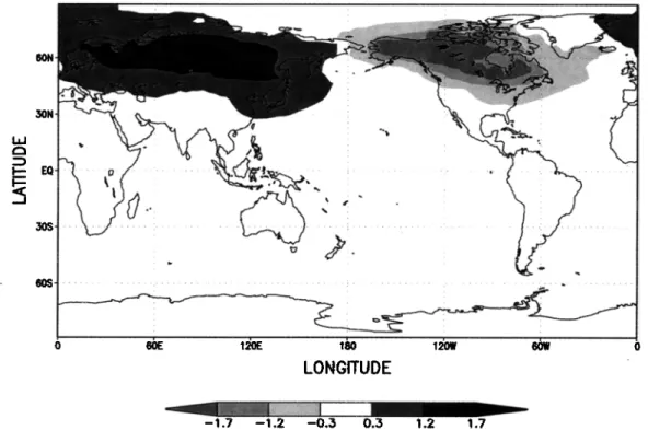
to the data.) The reason for the occurrence of counteracting flux estimates is that zonal mixing in the troposphere is much quicker than latitudinal mixing. Hence the footprints for fluxes from different regions within one zonal band may be almost indistinguishable. Consider, for example, the difference of the annual mean spatial mixing ratio distribution with reference to

the South Pole for fluxes from the North America boreal and

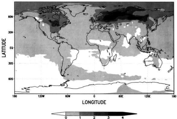
Eurasia boreal regions, respectively, in Figure 1. These two signals differ significantly from each other only within and next to the flux regions. Because of this, if CO2 concentrations were observed along the dateline only, the signals from fluxes from these two regions would be almost indistinguishable. Under these circumstances, the inversion procedure would become unstable, and estimates would be of unrealistically large mag- nitude [Tikhonov and Arsenin, 1977; Golub and Van Loan, 1989].

The second possible reason for failure of inversions is the presence of systematic errors, which might be induced by the

GLOOR ET AL.: INVERSIONS FOR SURFACE EMISSION CONTROL 14 247 60N 3ON 60S ;oE' ' ' =bW ... ... O LONGITUDE -1.7 -1.2 -0.3 0.3 1.2 1.7

Figure 1. Difference of the mixing ratio distribution ("footprint") (ppm) for fluxes from Eurasia boreal and

North America boreal.

assumptions and approximations needed to set up the prob- lem. For an inversion method based on annual mean mixing ratios, these approximations include (1) the simulation of at- mospheric transport by a model, which assumes that (a) trans- port processes like ventilation of the planetary boundary layer (PBL) and interhemispheric transport are correctly repre- sented and (b) synoptic and interannual variability of transport affect estimates only marginally, and (2) the prescription of specific spatiotemporal flux patterns (4)r : (4)r('0, (4), t) to simulate the footprints A Xr(X) for the inversions. For example, the spatial pattern of biospheric exchange fluxes may be mod- eled proportionally to satellite measurements (normalized dif- ference vegetation index (NDVI)), which may be close to the truth but may also be in error.

These approximations may have two consequences. First, estimates may be biased. Unrealistically low ventilation of the PBL, for example, will cause a systematic underestimation of fluxes if use is made of surface stations only. Second, there will be additional uncertainty in the estimates over that caused by mixing in the atmosphere alone. If, for example, there is a mismatch between real spatiotemporal flux patterns and those used to simulate the footprints, the differences will be misin- terpreted by the inversion. These differences will effectively add to and increase the estimated natural high-frequency vari- ability of the data.

To assess the value of inversions for flux monitoring pur- poses, the magnitude of all these possible errors will be esti- mated here. One major emphasis of this investigation is to use

a method which avoids the convolution of the effect of various

error sources and which is independent from a specific obser- vation network. To achieve this goal, we adopt a Monte Carlo approach that generates ensembles of observation networks with randomly positioned observation stations to obtain en-

sembles of estimates. From these ensembles, we calculate

mean estimates and standard deviations. We base our analysis on the inversion method that we have already discussed. To simulate the footprints AXr(X), we use two atmospheric trans- port models (SKYHI and global chemical transport model (GCTM), both developed at Geophysical Fluid Dynamics Lab- oratory/National Oceanic and Atmospheric Administration (GFDL/NOAA)), and use either spatially uniformly distrib- uted flux patterns or fossil fuel flux patterns. We then use these footprints to invert "pseudo-observations" obtained from sim- ulations with various models of fossil fuel burning, oceanic fluxes, land biosphere net primary productivity and respiration, and SF 6 emissions.

In the first part of the paper, we concentrate on the relation

between the number of measurement stations and the number

of source flux regions which they permit to estimate to a given accuracy, if there were no systematic errors. To achieve this goal, we use the expression for the error propagation for a linear inversion problem and the measured high-frequency data variability of the measurements of NOAA/Climate Mon- itoring and Diagnostics Laboratory (CMDL) as reported by Conway et al. [1994].

In the second part, we quantify biases caused by all the, approximations listed above that are needed for inversions

based on annual mean observations. We select suitable simu-

lations for the inversions and the pseudo-observations such that estimates are only affected by one source of error at a

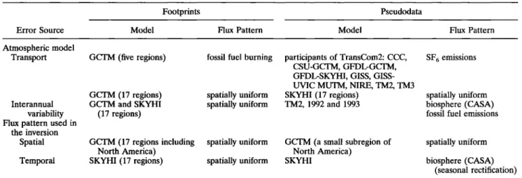
time. Table 1 summarizes our choice of combinations of inver-

sion schemes and pseudo-observations. We estimate the mag- nitude of the errorin modeled transport in two ways. First, the emissions of SF 6 are estimated from the simulations of all 12 models that participated in the model intercomparison study TransCom2 [Denning et al., 1999]. We base the inversions on the GLOBALVIEW-CO2 network [National Oceanic and At- mospheric Administration, 1997] (Also available on Internet via

Table 1. Choice of Combinations of Footprints and Pseudodata to Evaluate the Magnitude of Errors Caused by the Error

Sources in an Inversion Based on Annual Mean Observations

Footprints Pseudodata

Error Source Model Flux Pattern Model Flux Pattern

Atmospheric model

Transport GCTM (five regions) fossil fuel burning participants of TransCom2: CCC, SF 6 emissions

CSU-GCTM, GFDL-GCTM,

GFDL-SKYHI, GISS, GISS- UVIC MUTM, NIRE, TM2, TM3 SKYHI (17 regions)

TM2, 1992 and 1993

Interannual

variability Flux pattern used in

the inversion Spatial Temporal GCTM (17 regions) GCTM and SKYHI (17 regions) GCTM (17 regions including North America) SKYHI (17 regions) spatially uniform spatially uniform spatially uniform spatially uniform GCTM (a small subregion of North America) SKYHI spatially uniform biosphere (CASA)

fossil fuel emissions

spatially uniform biosphere (CASA)

(seasonal rectification) CCC, Canadian Climate Centre general circulation model; CSU-GCTM, Colorado State University general circulation model; GFDL-GCTM, Geophysical Fluid Dynamics Laboratory global chemical tracer transport model (Princeton, New Jersey); GFDL-SKYHI, Geophysical Fluid

Dynamics Laboratory general circulation model; GISS, NASA-GISS tracer transport model; GISS-UVIC, GISS-UVIC tracer transport model; MUTM, Melbourne University tracer model; NIRE, NIRE tracer transport model; TM2, tracer model version 2; TM3, tracer model version 3,

CASA, Carnegie Ames Stanford Approach; and SF6, sulfur hexafluoride.

anonymous FTP to ftp.cmdl.noaa.gov, Path: ccg/co2/ GLOBALVIEW) and fossil fuel flux patterns. These are sim- ilar to the flux patterns of SF 6 because both are strongly tied to energy consumption [Denning et al., 1999]. Second, we deter- mine transport errors with the two conceptually identical in-

version schemes of GCTM and SKYHI and relate them to

differences in model transport. We address the errors caused by neglecting the interannual variability of atmospheric trans- port by inverting the simulations of the annually repeating Carnegie Ames Stanford Approach (CASA) biosphere and fossil fuel emissions from different model years and comparing the difference of the estimates (the emissions themselves do not vary from year to year.) We determine the errors caused by differences between the flux patterns used to simulate the footprints for the inversion and the flux pattern that caused the actual mixing ratio distribution by inverting the mixing ratio distribution that results from a highly localized source within North America. North America itself is one of the flux regions used to simulate the footprints for the inversion. Finally, to estimate the biases induced by the neglect of the covariation of the seasonal cycle of fluxes with transport in an inversion based

on annual means, we invert the annual mean mixing ratio

distribution caused by a balanced biosphere (i.e., a biosphere with zero annual flux) predicted by CASA. A balanced bio- sphere is suited for this purpose because of its strong seasonal cycle.

2. Methods for Error Estimation

2.1. Amplification of High-Frequency Data Variability by the Inversion Process

Dilution of flux signals by mixing in the atmosphere leads to uncertainty of flux estimates because of amplification of the natural high-frequency variability in the data. To quantify the uncertainty of flux estimates due to this error source, it is helpful to arrange the footprints of regional fluxes, sampled at a specific network, in a matrixA = {AX• , ..., AXe}. The ith component of the vector AXr is the annually averaged mixing

ratio (with respect to a reference station) observed at station i

for a tracer emitted from region r. The matrix A maps a specific combination of regional fluxes to the observed spatio- temporal pattern: A x = A h. Correspondingly, the flux contri- butions to an observed signal in units of 4>r are obtained from

its pseudo-inverse by •t = A-•AX [Golub and Van Loan,

1989]. The variance-covariance matrix of the flux estimates,

C•,, may now be expressed in terms of the pseudo-inverse of A and the covariance matrix of the data C ax as C•, -

A-•C•xx(A-•) r. The diagonal

elements

of C•, and

C•xx

are

the variances of the flux estimates and the data, respectively. The off-diagonal elements are the correlation of estimates from different regions and data from different observation stations to each other, respectively. There are hence two parts

which contribute to the uncertainty of estimates: the data co-

variance Cax and its amplification, which is given by the ma-

trices

A - • and (A - •) r which

bracket

Cax. The matrix

ErrAmp -= A-•(A-•) r, with units

(Pg C yr -• ppm-•)

2, is

called the error amplification matrix [e.g., Menke, 1989]. This matrix is independent of any assumptions on data uncertainties and hence reflects exclusively atmospheric transport properties

and the choice of sites and number and location of source

regions. It is one decisive piece of information for the deter-

mination of the detection limit of fluxes with an inversion method. Writing out its diagonal elements, ErrAmpr r = •= 1

(•SCkr/15AXk)(•SCkr/15AXk), helps to clarify its meaning: they are

the sum over all observation stations of the sensitivities of the

flux estimate of region r to changes in data. Finally, an overall measure for the amplification of high-frequency data variabil-

ity is the average

over all regions'

(l/R) •rR=l ErrAmprr,

which we will call mean error amplification.

2.2. Method to Estimate Systematic Errors and Amplification of High-Frequency Data Variability Independently From a Specific Network

Let us assume for the moment that the mixing ratio distri- bution observed in the atmosphere is the one from fossil fuel emissions, AX•(x ), and that we would like to estimate the regional fluxes that caused A Xee(x ) with an inversion. Let us further assume that we have no preconception of the spatial

GLOOR ET AL.: INVERSIONS FOR SURFACE EMISSION CONTROL 14,249

30S-

ß ß

•r f .... "

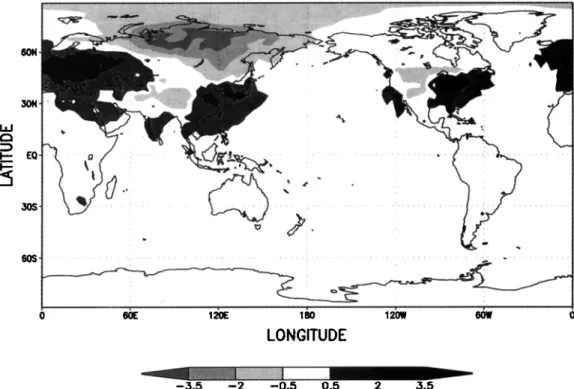
Figure 2. Difference between the mixing ratio distribution resulting from the linear superposition of the regional footprints (simulated using spatially uniform flux patterns) multiplied by the annual regional fossil

fuel

emissions

(tbrr

r •rRf_11

y

....

gionr•FF

der

dt)

and

the

mixing

ratio

distribution

resulting

from

fossil

fuel

emissions

(AXvv(.x)}: •)FF,rAXr(X)

-- AXFF(X

).

pattern of these fluxes so we choose spatially uniform fluxes to

simulate the footprints for the inversion. The resulting smooth mixing ratio distributions contrast drastically with the fossil fuel mixing ratio distribution, which exhibits very large local maxima at the main industrial regions, since the emissions are

strongly concentrated there. Accordingly, it is not possible to represent exactly the fossil fuel mixing ratio distribution in the atmosphere as a linear combination of the footprints, and the estimate of fossil fuel emissions will be biased. To illustrate this

point,

consider

in Figure

2 the difference

5;r• 1 tk•,r A Xr(X) --

A Xvv(x ) between the mixing ratio distribution, which results

from the combination 5? _{r= 1 <•)FF,rA Xr(x) of regional footprints}

generated by homogeneously distributed fluxes multiplied with

the regional

fossil

fuel emissions

(tb•.r --- fRegion

r•FF('O, •)

der dt), and the actual fossil fuel footprint AXvv(x ). Near the

industrial centers the approximation of the fossil fuel mixing ratio distribution with those based on homogeneously distrib- uted sources is poor. As a consequence, stations positioned there will drastically misinterpret the local signals, and the estimates will be unprecise. Typically, estimates based on

pseudodata sampled at a concrete observation network like

GLOBALVIEW-CO2 indeed deviate strongly from true fluxes

(here fossil fuel). Nevertheless these estimates convolute dif-

ferent causes of errors with each other. For example, it is unclear how much of the disagreement is due to the limited,

possibly insufficient size of the network, how much due to the specific positions of the observation stations, and how much is

really due to spatial mismatch. One needs a methodology that

permits one to distinguish the contributions of these various

error causes to a flux estimate, and furthermore, one would

like to determine biases, like the one caused by spatial mis- match, independently from a specific observation network.

For this reason, we use here a Monte Carlo approach which positions observation stations randomly to generate ensembles of estimates. To determine biases caused by systematic errors, we specifically proceed as follows. First, we determine a mean flux estimate from a particular footprint AX(X) used as pseudo-

observation (e.g., the one resulting from fossil fuel emissions)

by taking the mean over an ensemble of N estimates based on

- • A X•. Here A

N random

networks:

4)mean

• (l/N) 5;i

N_

• A i

i

is the map between regional fluxes and observations for the ith random network and AX• are the values of the pseudo- observations. The mean estimate 4)mean will generally differ from the true fluxes because of the differences of the spatial structure of footprints and pseudodata. The difference be-

tween the mean estimate and the true fluxes then is the bias:

4)bias • 4)mean -- 4)t .... where 4)true are the "true" fluxes that were used to generate the pseudo-observations. Mean esti- mates, determined as described, are found to be essentially independent from the fixed number of stations used, as long as they encompass no less than 50 stations.

Similarly, we may measure the enhanced scatter of estimates caused by differences of the spatial structure by the standard

deviation of the estimates of the ensemble of random net- works:

STDr=

(N- 1) • ((•)i,r--

I])mean,r)

2 ,

where tb•,r is the estimate of the flux from region r based on the

randomly chosen network from the i th draw. For the example above, for instance, one expects large scatter of the estimates

of fluxes from the main industrial centers if based on networks

agreement between the footprints and the fossil fuel mixing

ratio there, and much less scatter of the estimates for the

remaining regions.

We use a similar approach to determine how much estimates are affected by the neglect of interannual variability of trans- port in an inversion. We determine mean estimates ((b .... ) for two different years with different atmospheric transport but identical biospheric and fossil fuel flux patterns simulated by TM2 (which is based on analyzed winds). To determine the maps A i, we use the footprints generated with source strengths that are spatially-uniformly-distributed. The difference be- tween the mean estimates ((b .... ) from different years gives us an estimate of the magnitude of the differences of estimates caused by the interannual variability of model transport. Al- though this use of two specific years may be criticized for its lack of generality, we obtained similar conclusions using two different years, and our main point is to estimate the order of magnitude of the biases and which regions are most affected.

For the determination of systematic errors, we generally use randomly generated networks with 150 observation stations because (1) --•150 stations are necessary to estimate fluxes on a continental scale (for 10-20 regions), if positioned randomly, to suppress the errors caused by the amplification of high- frequency data variability; (2) because systematic biases man- ifest themselves strongly if inversions are based on small net-

works with 40-80 stations but there is a "saturation" level from

which point on biases do not decrease much further with ad- ditional stations; for the estimation of 10-20 regions this sat- uration level is reached at --•150 stations, and (3) because for the large number of 150 stations, networks with randomly positioned stations are almost as efficient as optimized net- works (cf. section 4.1).

Finally, to determine the relation between estimate uncer- tainty and number of observation stations, we average the mean amplification of high-frequency data variability over ran-

dom draws of observation networks with a fixed number of

stations (section 2.1):

N

• ErrAmp•?

.

i=1 r=l

3. Description of Models, Simulations, and

Footprints AXr(X )

3.1. Model Characteristics

The off-line atmospheric transport model GCTM [Mahlman and Moxim, 1978] developed at GFDL/NOAA is driven at a time step of 26 min by linearly extrapolated 6-hour time- averaged, annually repeating climatological winds. These were originally simulated by a modified, seasonally varying version of ZODIAK [Holloway and Manabe, 1971]. GCTM has no diurnal physics. It solves the tracer transport equation on 11 sigma levels, extending from Earth's surface to about 30 km height. The centers of the lowermost layers lie at 0.08, 0.5, 1.5, and 3.1 km height. Horizontally, an equal-area grid with an --•265 km x 265 km box size is used. Vertical subgrid-scale transport is parameterized by an eddy diffusion coefficient, which takes mixing due to velocity shear, as well as convection in case of unstable density profiles, into account. In addition, within the PBL, a mixing length scheme with decreasing mixing

length from the lowest to the third model layer is added [Levy

et al., 1982, 1989]. The mixing lengths for these three levels

have

been

adjusted

so as to match

222Rn

profiles

compiled

by

Liu et al. [1984].

The atmospheric general calculation model (AGCM) SKYHI [Fels et al., 1980], developed at GFDL/NOAA, calcu- lates tracer transport on-line, has 40 vertical levels extending from the surface up to --•80 km, uses a hybrid pressure-sigma coordinate in the vertical, and has a diurnal cycle of solar radiation. The horizontal grid is regular, and the resolution used for this study is 3 ø longitude by 3.6 ø latitude. There are eight layers between the surface and 5.2 km height, the lower-

most ones centered 0.08, 0.27, 0.74, and 1.38 km above Earth's

surface. The parameterization of vertical mixing in the PBL in SKYHI differs from that of GCTM: in case of potential tem-

perature inversions, the vertical diffusion coefficient is set to

the maximal value that does not cause numerical instability. A detailed description of SKYHI and its climatology is given by Hamilton et al. [1995].

The transport core of the TM2 model derives from the Goddard Institute for Space Studies (GISS) tracer transport model version of Russell and Lerner [1981], and European Centre for Medium-Range Weather Forecasting (ECMWF) analyzed winds are used to drive tracer transport off-line [Heimann, 1996]. The model grid encompasses nine layers in the vertical, extending from the ground up to 1 mbar (lower- most layers 0.22, 0.8, 1.85, 3.56, and 5.86 km), and the hori- zontal resolution is 8 ø latitude by 10 ø longitude, which is much coarser than that of both GCTM and SKYHI. Subgrid-scale transport is simulated by a cumulus cloud convection scheme, and vertical diffusion in the PBL is parameterized in a similar

way as in GCTM.

References for the models participating in TRANSCOM2 are given by Denning et al. [1999].

3.2. Footprint Simulations

We simulated two different types of footprints, AXr(x), r = 1, ..., R, for the inversion schemes: one type with spatially uniform flux patterns (within a region) and another type with the flux pattern of fossil fuel burning. For the first type, we build the following sets by combining or partitioning the foot- prints of 17 basic regions (Figure 3): (1) 11 source regions: Eurasian boreal and Eurasian temperate combined, North American boreal and temperate combined, Indian Ocean trop- ical and temperate combined, Atlantic tropics and South At- lantic temperate combined, Australasia, Pacific tropics, and South Pacific temperate combined, and all remaining 17 re- gions by themselves; (2) 22 source regions, including five ad- ditional regions, which result from splitting South America, Africa, South Pacific temperate, Australasia, and North Pacific

temperate in two parts (Figure 3); and (3) 25 regions (focus on

North America): N. American boreal and temperate split up in 10 subregions. For the second type, we simulated footprints with the pattern of fossil fuel emissions from five regions: North America boreal and temperate, Eurasia boreal and tem-

perate, and the combination of South America, Africa, and Australasia.

For use as pseudo-observations, we simulated mixing ratio distributions for the following flux patterns: fossil fuel emis- sions for the year 1990 [Andres et al., 1996], estimated oceanic fluxes [Takahashi et al., 1997], and estimates of land biosphere net primary productivity and respiration derived from satellite measurements (NDVI [Potter et al., 1993]). Each of these pseu-

do-observations have been simulated with GCTM, SKYHI, and TM2. We also use the simulations of the distribution of

GLOOR ET AL.: INVERSIONS FOR SURFACE EMISSION CONTROL 14,251

90N" ' ß

&

• Atlantic

Pola• '

60N

ß • ;"A•:T:mefica:

• ....

Xwr-

•" '? ':':

.... :Eu•l'a?Børe"•

•.. -'•'"•'

"'"'•

I ' - " ... • /• •. - '"- ... •' ...

•

. ß

•..

• N Amen• • ....

..:--:;.--

;:

;:.

-- - - •- •;.-..-:.

.... -•.-.--

I =

•••Tem•rat•.-.Af(:...•.

•-•...•'

•

: ePacific

Tro_ics

•'•,• Atlantic•-

:%': T•lndia•

• 0 -e

P • •"-:S:•:/•-:-

•. Tropics

--• ;;• eTropi•

••

•

-

• •,• ' S•Pacific-

' / S Atlantic

•. •/• F S Indian t

•' '•'"•'"

•o- T•maerate

• T••• '•• Temperate

- .

60S Southem Ocean

90S

180 120W 60W 0 60E 120E 180

LONGITUDE

Figure 3, Partitioning of Earth's surface in •cgions used fo• the inversion schemes.

SF 6 in the atmosphere from the participants of TransCom2 [Denning et al., 1999].

3.3. Relation Between Footprints •Xr(X)

and Model Transport Properties

Annually averaged surface mixing ratio distributions due to

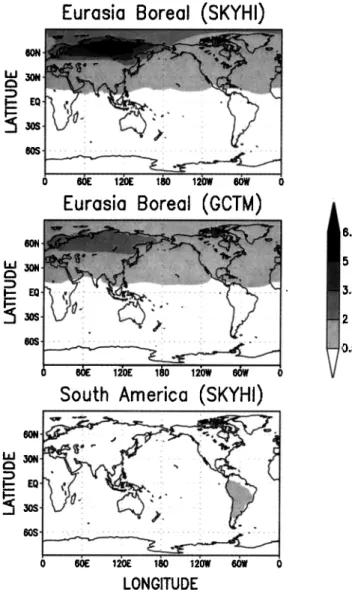
regional fluxes (Figure 4) may be conceptualized as a super- position of an approximately zonally symmetric "background"

field, reflecting the predominance of zonal winds and related rapid zonal mixing in the troposphere, and a strong, "regional"

signal within the flux region itself, determined by the ventila-

tion rate of the PBL. Background fields exhibit interhemi-

spheric

'slopes

in the surface

layer

between

_+2

ppm

Pg C -•

yr-•, and

regional

signals

vary

from

2 to 4 ppm

Pg C- • yr- • for

the northernmost

continents

to 1-1.2 ppm Pg C -• yr -• in the

midlatitude

regions,

and to 0.6 ppm Pg C -1 yr -1 in tropical,

continental regions where convective ventilation of the PBL is largest.

The magnitude of the regional signal differs considerably between SKYHI and GCTM, but the spatial structure (i.e., form of isolines) is almost identical; the background fields are also similar. Some signals resulting from fluxes from a bounded region at Earth's surface as simulated by GCTM and SKYHI are shown in Figure 4. For most regions, regional annual-mean surface mixing ratios simulated by SKYHI are lower than those simulated by GCTM, with the exception of the three north- ernmost regions: North Atlantic polar, Eurasian boreal, and North American boreal. There, surface mixing ratios simulated by GCTM are smaller by about 50%. The reason for these discrepancies is that the PBL ventilation simulated by SKYHI

is stronger than that by GCTM for most regions (for the reason

explained in section 3.1). The exceptional regions are the northernmost ones, for which SKYHI predicts near-ground inversions during winter and hence surface fluxes are trapped, resulting in high surface concentrations. The resolution of the

PBL of ZODIAK, from which the off-line winds for GCTM derive, is too coarse to resolve such wintertime inversions, and

the PBL ventilation rate is therefore much larger there. Raw- insonde data from these regions support the simulations of

SKYHI.

Results of inversions based on zonally averaged models rely strongly on the interhemispheric gradient resulting from asym-

metric

fluxes

in both hemisphereS.

The magnitude

of this in-

terhemispheric gradient for fixed source strength depends both on the efficiency of PBL ventilation and interhemispheric mass exchange. We use a simulation of the CO2 distribution result- ing from fossil fuel emissions to compare the models. The zonally averaged interhemispheric gradient resulting from fos- sil fuel burning for 1990 [Andres et al., 1996] as simulated by GCTM is larger than that by SKYHI by -10-15%, whereas the latitudinal structure is similar (the interhemispheric ex-

change times are 0.8 and 0.9 years, respectively). The zonally

averaged interhemispheric gradient from pole to pole as sim- ulated by TM2 is similar to that by GCTM, whereas in the northern midlatitudes the mixing ratios are smaller than in GCTM by -15-20%. An intercomparison study by Law et al. [1996], which encompassed 11 other models as well, showed that the interhemispheric gradient simulated by GCTM caused by fossil fuel emissions is larger in the midlatitudes of the Northern Hemisphere compared to most other models. A large part of the discrepancy is attributable. to the higher spa- tial resolution of GCTM, which permits much larger spatially localized signals compared to the remaining models (compare with Denning et al. [1999, Table 1 and Figure 4]).

4. Evaluation of Error Sources 4.1. Relation Between Estimate Uncertainty

and Number of Observation Stations

An essential concern in applying inversions to the monitor- ing of surface fluxes is a determination of the minimum num-

ber of stations needed to estimate fluxes to a reasonable ac-

curacy for a given number of regions. Also of interest is the maximum number of regions for which surface fluxes may be

Eurasia

Boreal

(SKYHI)

i.i:...::.'.i

.... .

...

•;• •05

South America

(SKYHI)

. . 5.5 6ON' LzJ ,]ON- I"" EQ-

• 3os,

60S

...

...

'

"'

'•••

"

Figure 4. Carbon dioxide mixing ratio distribution (ppm)

with reference to the South Pole for a flux from Eurasia boreal

simulated by (top) SKYHI and (middle) GCTM, and (bottom) a flux from South America simulated by SKYHI.

estimated to satisfying accuracy, given a fixed number of ob- servation stations (the "spatial resolvability" of the method). To determine average flux estimate errors from amplifica- tion of high-frequency data variability (with the formula

.A-1CAx(.A-1)

T) (section

2.1)), one needs

an estimate

of

high-frequency

data

variability

(the diagonal

elements

of Cax)

as a function of latitude and longitude. We cannot rely on our model simulations for these estimates because our biospheric model has no daily cycle of biospheric fluxes. Here we will instead use the variability in the available observations. Guided by the magnitude of observed variability, two types of obser- vation stations, "continental" and "remote," positioned on is- lands in the oceans, are usually distinguished. High-frequency data variability for remote stations were reported by Conway et al. [1994]. Standard deviations of annual mean data from the year 1992 are mostly of the order of 0.1-0.2 ppm, with the exception of three stations (maximal standard error for Cape Meares, rr • 0.3 ppm, where winds loaded with pollutants occasionally blow from the land). Data variability at continen- tal stations in temperate and boreal ecozones is larger. For

example, Bakwin et al. [1995] report mixing ratios from mea- surements on a very tall tower in North Carolina. Monthly standard deviations of daily mean CO2 mixing ratios at 496 m height are of the order of 4 ppm. The standard error of the annual mean mixing ratio accordingly is ---1.2 ppm, the value that we adopt in the following for continental stations.

Consider in Plate 1 (left panel) the dependence of the am- plification of high-frequency data variability on the number of observation stations and flux regions. For all surface partition- ings the decrease of the mean error amplification with increas- ing amount of stations is dramatic for small networks of up to ---150 stations and modest for larger ones. Installation of more than 150 monitoring stations on a continental scale (i.e., solv- ing for 10-20 flux regions) is hence not very helpful because uncertainties decrease only very marginally. The decrease fol-

lows

---1/V• (i.e., like statistical

counting

error),

where

N is

the number of observation stations. The level of amplification of high-frequency data variability for large networks is not sensitive to the number of flux regions used for the inversion.

Conversely, these curves show that trying to estimate fluxes from more regions than approximately a tenth of the number of observation stations is not possible (at least if stations are positioned randomly) because the flux errors caused by the amplification of high-frequency data variability alone (not to mention systematic errors) in that case reach uncertainties of 1

Pg C yr -• region

-1 (the product

of the value

of error ampli-

fication with the value of high-frequency data variability), which makes the solutions useless for most purposes.

Finally and most important, for an intermediate value of high-frequency data variability of 0.5 ppm for each of 150 stations used to estimate fluxes from 10-20 regions, the am- plification of high-frequency data variability for the estimation

of fluxes results in errors of the order of 0.2-0.3 Pg C yr -1 region -1 (the product of the mean error amplification ---0.5 Pg C yr -1 ppm -1 region -1 with the level of high-frequency data

variability ---0.5 ppm). Note that a larger value of---0.4 Pg C

yr -1 region

-1 is obtained

if only

remote

stations

are used

(for

which the high-frequency data variability is only 0.2 ppm, but

the mean

error amplification

is 1.9 Pg C yr -• ppm

-1 region-1).

number of regions to be estimated, as far as amplification of high-frequency data variability is concerned, is therefore ---10; monitoring of CO2 exchange fluxes would thus be feasible with a fairly reasonable measuring effort.

The amplification of high-frequency data variability in- creases strongly with height because information on fluxes fades away quickly with increasing distance to the ground. We find approximately a fivefold increase between 0 and 5 km height, and a 20-fold increase between 0 and 10 km height. The profile of error amplification with height over Earth's surface was determined for layers centered at 0.08, 0.5, 1.5, 3.1, 5.5, 8.7, and 12 km height and using the same method as described in section 2.2. The values are global averages. This result means that airplane transects at high altitudes (>-5 km) are not effi- cient in constraining inversions to estimate surface fluxes. It is important to notice what this result does not imply. First, high-altitude transects may well be of considerable value in constraining the modeling of atmospheric transport, as sug- gested for example, by the results of the model intercompari- son study TransCom2 [Denning et al., 1999]. Second, the result is restricted purely to high-altitude transects and is not valid for vertical profiles extending to the earth surface.

GLOOR ET AL.' INVERSIONS FOR SURFACE EMISSION CONTROL 14,253

F 102

E

o) 0 •

13..

1

x 11 Regions

ß 17 Regions

o 22 Regions

+ 25 Regions

o 17 Reg- Rem. Sts.

ß 17 Reg - Opt. Sts.

• 10ø

I!

•e!•

- )

Observation Stations

• 01

'-1

• 0

0

E

10

-1

Observation

Stations

Plate 1. (left) Average

error amplification

((l/R) ErR=i

ErrAmprr)

1/2) and (right) average

bias for the

estimation of fossil fuel emissions for an inversion scheme based on a uniformly distributed flux from Earth's surface as a function of the number of observation stations for various partitionings of Earth's surface. The determination of the averages over random networks is described in section 2.2. The red curve was obtained permitting only stations in the oceans, and the black dots were determined with an algorithm that places stations optimally for the estimation of surface fluxes with minimal uncertainty.

toward random networks with increasing number of observa- tion stations. An optimized network with 40 stations is ---10 times more efficient in constraining sources and sinks com- pared to a randomly positioned network for the estimation of 17 regions, whereas an optimal network with 160 stations (for which the mean error amplification is minimal) is only mar- ginally superior to a random network (by ---25%). This is one of the justifications for the use of 150 stations for random networks as a basis to determine the magnitude of systematic biases. Optimal networks were determined by minimizing the uncertainty of estimates, given a best estimate of high- frequency variability. The optimizations were performed with the simulated annealing algorithm [Kirkpatrick et al., 1983]. For a more detailed discussion, we refer to M. Gloor et al. (Opti- mal network design for the purpose of inverse modeling: A model study, submitted to Global Biogeochemical Cycles, 1999).

The decline of biases with the number of stations is illus-

trated in Plate 1 (right panel) for the same example as in section 2.2: the recovery of fossil fuel emissions with an inver- sion based on spatially uniform fluxes. The main feature here

is that there is a saturation level for the number of stations,

above which biases do not decrease any further with additional

stations. For the estimation of 10-20 regions, this level is approximately reached with 150 stations, which is the second of the justifications mentioned in the Introduction to base our analysis on 150 observation stations.

4.2. Relation Between Atmospheric Transport and Regional Flux Estimate Uncertainty

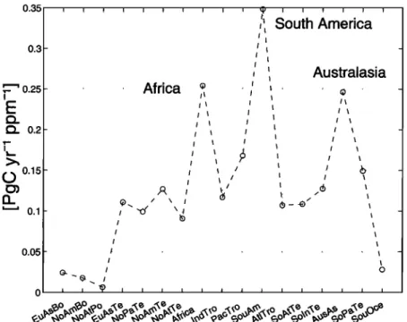
The Monte Carlo approach applied to regional error ampli- fication permits one to identify the regions with largest infor- mation loss (Figure 5). For the 17-source region partitioning,

these are South America, Africa, Australasia, and to a lesser

extent, Eurasia temperate. Further subpartitioning of the first three regions into tropical and subtropical zones reveals that the weakest constrained regions are equatorial South America, equatorial Australasia, and equatorial Africa (the average er- ror amplifications for Africa, South America, and Australasia

are 0.31, 0.54, and 0.32 Pg C yr-• ppm-• region-•, respective-

ly). As mentioned above, fluxes from continental, equatorial regions, result in comparably small signals within the source region itself. This is due to strong convective ventilation of the PBL. The regional error amplification is hence inversely re- lated to the regional signals. This simple result illustrates that what really determines the amplification of high-frequency

2.5 ß c 1

ß 0.5

E

Plate 2. Estimates of SF 6 emissions from footprints simulated with 12 different transport models for North America temperate and boreal, Eurasia temperate and boreal, and South America, Africa, and Australasia combined. The observation network is GLOBALVIEW-CO2, and the inversion uses fossil fuel footprints. See Table l footnote for acronyms.

I I I I ! I I I I Inversion Prediction o o o o • .•o • o • •o • •

1.6

o

Plate 3. Average estimates of fluxes of 1 Pg C yr-• region-] simulated in SKYHI and estimated with the

inversion scheme of GCTM and 150 observation stations The flux patterns used for the inversion with GCTM are identical with those in SKYHI used to generate the data mixing ratio fields. Average estimates are aligned

horizontally for a flux of 1 Pg C yr-] for each of 17 regions listed on the y axis at a time and a flux of 0 Pg C yr-• from the remaining regions.

GLOOR ET AL.' INVERSIONS FOR SURFACE EMISSION CONTROL 14,255 0.35 0.3 ,- 0.25 I E c.• 0.2 I•._

(,• 0.15

,', South Arneric8

I

I

•

I

/

Figure 5. Average error amplification for each of the 17 source regions of Figure 1 and an observation network encompassing 500 observation stations. The determination of the average over random networks is explained in section 2.2.

data variability and hence a lower bound for the flux detection limit of the inversion is the intensity of tropospheric mixing. It also implies that the continental, equatorial regions need higher data coverage than others for equally trustworthy flux estimates.

4.3. Systematic Errors

4.3.1. Errors caused by differences of modeled transport.

Estimates of fluxes from inversions are biased, in part, because modeled transport differs from the true transport. To get a handle on the magnitude of these errors, given the state of art of atmospheric transport modeling, we estimate SF 6 emissions from mixing ratio distributions simulated by 12 models, based on an identical flux pattern. We then analyze in greater detail the relation between errors and transport differences for the

two models GCTM and SKYHI.

The simulations of SF 6 mixing ratio distributions were per- formed during TransCorn2 [Denning et al., 1999], a model transport intercomparison study. We estimated the SF6 emis- sions using fossil fuel footprints calculated with GCTM for the following five regions: Eurasia boreal, Eurasia temperate, North America boreal, North America temperate, and all re- maining continental regions combined. We use the simulations of emissions from fossil fuel burning with GCTM. As the observation network, we use GLOBALVIEW-CO2 [NOAA, 1997] (also available on Internet via anonymous FTP to ftp. cmdl.noaa.gov, Path: ccg/co2/GLOBALVIEW). the largest self-consistent data set of CO2 observations currently available.

The estimates of SF6 emissions derived from each of the 12 TransCom2 model SF 6 results are shown in Plate 2. Note that differences between flux estimates and the true emissions are

of the same order of magnitude as the emissions themselves. The reason for this is mainly attributable to different transport properties of the models because 66 stations (the number of observation stations of GLOBALVIEW-CO2) are enough to reduce the error from amplification of high-frequency data variability to an insignificant level (cf. section 4.1).

In the case of the GCTM SF 6 overestimate of the flux from Eurasia boreal, the reason cannot be transport because the SF 6

mixing ratio distribution and the fossil fuel footprints are both

simulated with GCTM. In this case the error is caused by the difference of the SF 6 emission pattern, based on electrical energy consumption and population density [cf. Denning et al., 1999] and the CO2 emission pattern, based on fossil fuel en- ergy consumption, cement manufacture, and population den- sity [Andres et al., 1996]. Differences are particularly large at the Westerland monitoring station (8øE, 55øN) next to the North Sea, where the fossil fuel emission pattern predicts com- parably smaller values than the SF 6 emission pattern, which in

turn, results in an overestimation of the Eurasian boreal flux. We next use SKYHI to generate pseudo-observations for

constant fluxes from each of 17 regions, and the footprints simulated with GCTM, based on exactly the same spatially uniform flux patterns, for the inversion to estimate the emis- sions in SKYHI. This procedure isolates the effect of model transport differences completely from all other sources of er- ror. In addition, to get error estimates independently from a specific observation network, we follow again the Monte Carlo approach described in section 2.2. We obtain annual-average estimates for the flux from each of the 17 regions from the inversion of each of the 17 mixing ratio distributions simulated by SKYHI for a spatially-uniformly-distributed flux of 1 Pg C

yr -•. For a given emission region these average estimates are

aligned horizontally in Plate 3. For example, the estimate of emissions in SKYHI from the Atlantic tropical region (line six)

attributes a flux of ---0.7 Pg C yr-• to Atlantic tropics, ---0.15 Pg

C yr- • to Pacific

tropics,

and approximately

_+0.05

Pg C yr-• to

all the remaining

r•gions.

If there

would

be no transport

error,

fluxes from the Atlantic tropics would be estimated to be 1 Pg

C yr -•, and 0 Pg C yr -• would be estimated for all other

regions. More generally, if there would be no difference in the transport properties between the two models, all diagonal el-

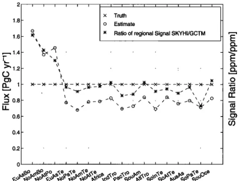
1.8 1.6 0.8 0.6 0.4 0.2 Truth Estimate

Rat!o of regional Signal SKYHI./GCTM

Figure 6. Mean estimates of SKYHI fluxes from 17 regions with the GCTM inversion scheme (diagonal elements of the matrix in Plate 2) and ratio of local signals of SKYHI and GCTM (cf. section 4.3.1).

ements in Plate 3 would be 1, whereas all the off-diagonal

elements would be zero. Most flux regions hence are correctly localized by the inversion scheme, with the exception of the

three northernmost and the southernmost ones.

A comparison of the ratio of the integrated "regional sig- nals" (the signals within the flux regions) as simulated by

SKYHI and GCTM (fregion

r/•,•SKYHI(X) dø'/fregionr

/•XOCTM(X) drr) for the case above (Figure 6) reveals the

following.

1. As long as the ratio of regional signals due to a regional flux is "small" (of the order of 10-20%), transport errors affect only the estimate of the flux from the flux region itself.

2. If differences of regional signals are of the order of 50%, as for the three northernmost regions, fluxes are misattributed to several regions. It is noteworthy, however, that the misat- tribution is only to other regions within the same zonal band as

the flux region itself.

3. Differences of estimates for the remaining regions may partially be explained by the ratio of the "regional signals" between GCTM and SKYHI (Figure 6) (---40% of the discrep- ancy) which are a result of stronger PBL ventilation in SKYHI and correspondingly smaller regional signals. The remaining discrepancy is attributable to different interhemispheric ex- change rates: SKYHI's exchange is more rapid by ---10%. Fluxes from the regions besides the northernmost ones are underestimated by approximately the same percentage. This result suggests that too rapid interhemispheric exchange will cause underestimates of the magnitude of fluxes for all regions and that the estimates scale inversely with interhemispheric

exchange rates.

4.3.2. Errors caused by the neglect of interannual variabil- ity of atmospheric transport. We estimate the magnitude of

biases and standard deviations of estimates caused by interan- nual variability by using footprints from one atmospheric trans- port model (SKYHI) for the estimation of fluxes from the atmospheric patterns simulated by two different model years of

another model (TM2). As footprints for the inversions, we use spatially uniformly distributed fluxes from 17 regions simulated by SKYHI; as pseudo-observations, we use the atmospheric patterns from fossil fuel emissions and biospheric exchange fluxes simulated by TM2. Note that TM2 is driven by analyzed winds, which differ from year to year while the fluxes are kept fixed from year to year. Differences of estimates from different years are not sensitive to the spatial patterns used for the inversions (here spatially uniform) because the estimates from the 2 years are affected in the same way by the specific choice of the spatial flux pattern, and their effect hence cancels out. As above, we base the inversions on randomly generated ob-

servation networks with 150 observation stations. The biases in this case are the difference between the mean estimates of the

2 years (as explained in section 2.2) and are tabulated in Table 2, together with the standard deviations of the estimates.

For biospheric fluxes, biases caused by interannual variabil-

ity are of considerable

magnitude

(.--0.2-0.3

Pg C yr -• re-

gion -•) for the regions where biospheric exchange fluxes are

large: Eurasia temperate, North America temperate, and Af-

rica (Table 2). Otherwise,

biases

are small

(-<0.05

Pg C yr -•

region-•). The standard deviations of the ensemble of esti-

mates, for a network with 150 stations, though, may be as large

as 0.5 Pg C yr-• region-•. For fossil fuel emissions, biases are --1

smaller than for the land biosphere; maximally ---0.2 Pg C yr

region-• (Table 2). Again, the standard deviations of the es- timates are somewhat greater, maximally 0.25 Pg C yr -• re- gion -•, and their mean is 0.1 Pg C yr-• region-•. A possible

way to reduce these biases and standard deviations might be

the use of a model with assimilated winds combined with a

time-dependent inversion scheme.

4.3.3. Errors caused by incorrect modeling of the spatial

flux pattern. To quantify the magnitude of systematic errors introduced by spatial differences between the flux patterns ½r(O, ½, t) used for the inversion and the real ones, we use the inversion scheme based on fluxes from 17 regions and, as