Calibration of the Meteosat water vapor channel using collocated NOAA/HIRS 12 measurements

HAL Id: hal-03120962

https://hal.archives-ouvertes.fr/hal-03120962

Submitted on 26 Jan 2021

HAL is a multi-disciplinary open access

archive for the deposit and dissemination of

sci-entific research documents, whether they are

pub-lished or not. The documents may come from

teaching and research institutions in France or

abroad, or from public or private research centers.

L’archive ouverte pluridisciplinaire HAL, est

destinée au dépôt et à la diffusion de documents

scientifiques de niveau recherche, publiés ou non,

émanant des établissements d’enseignement et de

recherche français ou étrangers, des laboratoires

publics ou privés.

Calibration of the Meteosat water vapor channel using

collocated NOAA/HIRS 12 measurements

Francois-Marie Bréon, Darren Jackson, John Bates

To cite this version:

Francois-Marie Bréon, Darren Jackson, John Bates. Calibration of the Meteosat water vapor channel

using collocated NOAA/HIRS 12 measurements. Journal of Geophysical Research: Atmospheres,

American Geophysical Union, 2000, 105 (D9), pp.11925-11933.

�10.1029/2000JD900031�.

�hal-03120962�

JOURNAL OF GEOPHYSICAL RESEARCH, VOL. 105, NO. D9, PAGES 11,925-11,933, MAY 16, 2000

Calibration of the Meteosat water vapor channel using

collocated NOAMHIRS

12 measurements

Francois-Marie Brdon • and Darren L. Jackson

Climate Diagnostic Center, Cooperative Institute for Research in Environmental Sciences, University of

Colorado, Boulder

John J. Bates

Climate Diagnostic Center, NOAA/ERL/CDC, Boulder, Colorado

Abstract. The Meteosat geostationary satellites carry a filtered radiometer channel

centered at 6.2 pm for the measurement of upper tropospheric humidity. The operational

calibration is derived from radiative transfer calculations applied to radiosonde

measurements; large fluctuations in the calibration have been noticed. Here, we apply

another method based on collocations with NOAA/High-Resolution Infrared Radiometer

Sounder (HIRS) channel 12. Radiative transfer calculations

show that Meteosat

measurements can be accurately predicted from HIRS channel 12 brightness

temperatures. In addition, the HIRS instrument has onboard calibration of the complete

optics, which makes it suitable as a reference for the calibration of other spaceborne

radiometers.

Application of the method to 3 years of Meteosat-5 data shows

calibration

fluctuations significantly smaller than those provided by the operational method. This

result indicates that the short-term stability of the instrument calibration is much better

than 5%, the variability given by the operational calibration.

The proposed

calibration

coefficient

is smaller by about 10-15%, which results

in equivalent

brightness

temperatures biased by about 3-4 K and 35-50% relative error on the upper tropospheric

humidity. Hypotheses of the causes for such large differences between the two calibration

procedure results are proposed.

1. Introduction

The Meteosat satellite series is one of the five geostationary satellites that provide nearly continuous coverage of the trop- ical and midlatitude areas, together with the Geostationary Operational Environmental Satellite (GOES) East and West, Geostationary Meteorological Satellite (GMS), and Indian National Satellite (INSAT). The Meteosat primary radiometer

carries three channels, one in the visible and near infrared, one

in the 11 •m thermal infrared atmospheric window, and one in the water vapor absorption band at 6.2 •m. The latter is de- signed to observe the upper tropospheric humidity and to track weather phenomena in the upper troposphere. Although the instrument was designed mostly for imagery, researchers have attempted more quantitative uses of the Meteosat measure- ments, which require accurate calibration [Van den Berg et al., 1991; Schmetz et ai., 1995; Roca et ai., 1997].

In this paper, we focus on the 6.2 •m water vapor channel. The onboard calibration procedure of the Meteosat instru- ment does not include the main optics and cannot be used for an absolute calibration of the water vapor channels. On the other hand, the TIROS Operational Vertical Sounder (TOVS) onboard the NOAA National Oceanic and Atmospheric Ad- ministration (NOAA) operational satellites is calibrated using

•On leave from the Laboratoire des Sciences du Climat et de

l'Environnement, CEA/DSM, Saclay, France. Copyright 2000 by the American Geophysical Union. Paper number 2000JD900031.

0148-0227/00/2000JD900031 $09.00

an onboard device. Moreover, it includes an upper tropo- spheric water vapor channel centered near 6.7 •m (High- Resolution Infrared Radiometer Sounder (HIRS) channel 12) which is similar to the Meteosat water vapor channel. This HIRS channel opens the way for possible calibration of Me- teosat using collocated measurements, as originally suggested by Beriot et al. [1982].

In section 2 we briefly present the operational calibration method. Section 3 presents some radiative transfer calculations

that indicate that the Meteosat measurements can be accu-

rately estimated from collocated NOAA/HIRS 12 observa-

tions. Section 4 describes an alternative calibration method

based on this finding. Section 5 shows the results of the method applied to 3 years of Meteosat-5 measurements. Section 6 discusses the results, and section 7 presents the conclusions.

2. Operational Calibration Method

The operational calibration method for the Meteosat water vapor channel is described by Van de Berg et al. [1995]. It makes use of radiosonde temperature and humidity profiles, given at standard isobaric levels (1000, 850, 700, 500, 400, 300, 250, 200, 150, and 100 hPa) for temperature and up to 300 hPa for humidity. A number of quality checks are applied to these data in order to reject doubtful measurements as well as dry sound- ings. The humidity profiles are linearly interpolated from the value at 300 hPa to 0% at 100 hPa. The profiles are used as input to a radiative transfer model that computes the atmo- spheric transmittance for six spectral bands distributed within the water vapor channel spectral band. The model provides an estimate of the top of atmosphere (TOA) radiance for the

11,926 BREON ET AL.' METEOSAT WATER VAPOR CHANNEL CALIBRATION 1 0.8

0.6

0.4

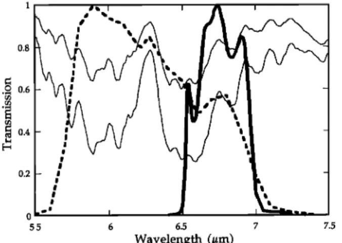
Figure 1. Spectral response of the NOAA 12/HIRS 12 (thick solid line) and Meteosat-5 water vapor channel (thick dashed line) instruments, together with typical atmospheric transmis- sion between the level 300 hPa and the top of the atmosphere for a midlatitude winter and a tropical profile (thin lines). The

former is larger than the latter. Absorption in this spectral

region, and therefore the atmospheric transmission spectral features, is mostly due to water vapor.

Meteosat spectral response. A simulated count is computed using the current calibration.

Meteosat measurements (32 x 32 pixels) around the radio- sonde stations are then extracted. A classification of the pixel measurements, using the IR window channel, is applied to separate clear and cloudy pixels. Measurements (numerical counts) from segments free of midlevel and high-level clouds are averaged. At this stage another quality check is applied, rejecting matchups that show a large difference between the

measured count and the simulated count derived from the radiosonde.

The remaining simulated radiances and the measured space count are used to compute the mean slope of the count- radiance relationship. This procedure is applied twice a day (using 0000 UT and 1200 UT radiosondes). The calibration coefficient is updated only if the new estimate differs from the current one by > 1%.

The random error of this method is estimated as 4% for individual radiosonde measurements; the error is further re-

duced by averaging the results of many collocations. We be- lieve, however, that this value is optimistic because several

sources of errors are not considered. Those error sources in-

clude the humidity profile vertical interpolation and extrapo- lation and the radiative transfer modeling. Also, the humidity measurement error from radiosondes appears to be underes- timated in the uncertainty analysis. Figure 6 of Van den Berg et al. [1995] shows the results of radiosonde and satellite mea- surement collocations and indicates that the scatter is signifi- cantly larger than 4%.

In the following we compare the results of our procedure to the operational calibration coefficients. These were acquired from the European Organization for the Exploitation of Me- teorological Satellites (EUMETSAT) web site at www.eumet-

sat.de.

3. Radiative Transfer Calculations

The Meteosat-5 water vapor channel and NOAA 12/HIRS 12 spectral responses are shown in Figure 1 together with two

typical atmospheric transmissions between the TOA and 300 hPa atmospheric level. Figure 1 shows that Meteosat has a much broader filter than HIRS 12, but they cover the same range of atmospheric transmission. One can thus expect that they yield similar measurements. Because the Meteosat filter is much broader, the integrated radiance measured by this in-

strument is larger than that of HIRS 12.

In order to evaluate the measurement variability for a wide

range of atmospheric profiles, we make use of the TOVS Initial Guess Retrieval (TIGR) [Ch•din, 1985; Chaboureau et al., 1998] version 3 database. In this database, radiosonde mea- surements have been quality checked and sampled so as to represent a very wide range of possible atmospheric condi- tions. The profiles are separated into tropical, midlatitude, and polar profiles. We did not make use of the polar profiles because the geographical coverage of Meteosat is limited in polar regions, which reduces the number of profiles to 1615. Radiative transfer calculations have been performed using the Modtran version 3.7 model [Wang et al., 1996] for both nadir and 60 ø view zenith angle. The model spectral resolution

is 1 cm -•, or about 4 x 10 -3/.•m. The simulated radiances are

spectrally integrated over the radiometer spectral responses.

For narrow filters, such as that of HIRS 12, the conversion

between radiance and brightness temperature is straightfor- ward using the Planck function and an equivalent wavelength:

L MODTRAN : P (T, Xeq)

f F(X)

dX, (1)

where LMODTRA N is the result of Modtran calculation, F(;t) is the instrument spectral response, P is the Planck function, and

;teq is an equivalent wavelength. The NOAA 12/HIRS 12

equivalent

wavenumber

of 6.763/xm

(1478.59

cm

-•) was

pro-

For a broader filter response, such as that of Meteosat, the choice of an equivalent wavelength is more difficult because of the nonlinearity of the Planck function with respect to both temperature and wavelength. EUMETSAT provides tables that relate radiance and brightness temperature, as well as an analytical fit to these tables. For the water vapor channel of

Meteosat-5, it reads

2266.7) (2)

L =exp 9.2361

T

'

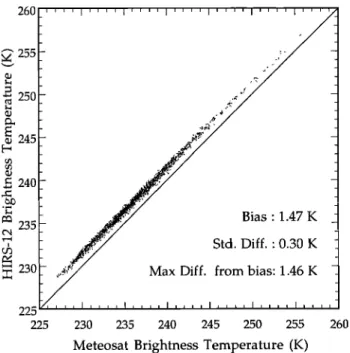
Figure 2 shows the results of radiative transfer calculations expressed as brightness temperatures (BTs). There is a very high correlation between Meteosat and HIRS 12 BTs. Meteo- sat BTs are slightly lower by about 1.5 K. One the other hand,

the standard deviation of the difference is only 0.3 K. These

results show that the two measurements are very similar and that the Meteosat measurement may be estimated from the

HIRS 12 measurement with a high accuracy.

Our objective is to derive a radiance calibration for the Meteosat water vapor channel. Therefore we seek a simple, yet accurate, relationship between the HIRS 12 measurement (ei- ther BT or radiance) and the Meteosat radiance. A relation-

ship that meets these criteria is

LMSAT = •-•P(BTHiRS ' (3) where fl and Xo are two parameters which were adjusted to minimize the residual. II is equal to 0.9146/.•m, which is close

BREON ET AL.: METEOSAT WATER VAPOR CHANNEL CALIBRATION 11,927

to the instrument-integrated transmission, and X o is 6.226 t•m,

which is close to the Meteosat channel center wavelength. Using these coefficients, there is no bias between the Meteosat radiances computed by MODTRAN and predicted from the HIRS BT. The relative difference is not greater than 3.52%, and its standard deviation is 1.21% (see Figure 3). The simu- lated and predicted radiances are generally colder for the 60 ø zenith angle than for nadir viewing, but there is no evidence of any systematic deviation from (3) as a function of the zenith

angle.

4. Calibration Method 4.1. Data

Three years (February 1994 to February 1997) of Meteo- sat-5 observations were provided by the Earth Observing Sys- tem Data and Information System (EOSDIS) Distributed Ac- tive Archive Center. There are a few gaps in data coverage. The original Meteosat measurements have been sampled to a resolution of ---30 km and with a time step of 3 hours from the original 5 km and 30 min spatial and temporal resolutions. In the International Satellite Cloud Climatology Project (ISCCP) B3 format, the data are given as numerical counts (between 0 and 255), and calibration tables are given to derive either radiances or BTs from the counts [Schiffer and Rossow, 1985]. Three levels of calibration are proposed: "nominal," "normal- ized," and "absolute." "Nominal" is the operational calibration provided by the agency responsible for the satellite (EUMETSAT in the case of Meteosat), and that is compared to our results

below. "Normalized" and "absolute" are derived so as to sim-

ulate measurements of the advanced very high resolution ra- diometer (AVHRR) for the visible and infrared window chan-

nels and simulate measurements of the HIRS 12 for the water

vapor channel. The procedure to derive normalized and abso-

260

255

250

245

22

••

Max

f. from

bias:

1.46

K

225 230 235 240 245 250 255 260

Meteosat Brightness Temperature (K)

Figure 2. Results of radiative transfer calculations using MODTRAN version 3.7 for 1615 tropical and midlatitude at- mospheric profiles for a viewing angle of 0 ø and 60 ø. The equivalent brightness temperatures have been computed for the two spectral responses shown in Figure 1.

1.2 ' ' ' ' I ' ' ' ß

• 1.1

.•m

0.6 /-.

at.

i .: 3

m /,

Mean

telat'

diff':

1'20

ø/ø

• 0.5

0.4

0.4 0.5 0.6 0.7 0.8 0.9 1 1.1 1.2

Meteosat

calculated

radiance

(W m -2 sr

-! )

Figure 3. Meteosat radiances derived from calculated HIRS

12 radiances, plotted against directly calculated Meteosat ra-

diances. The radiative transfer calculations are the same as

those shown in Figure 2, while the simulated radiances were calculated using equation (3).

lute calibration tables is described by Desormeaux et al. [1993]. In the following we make use of the numerical counts only.

The HIRS data originates from TOVS level lB data ac- quired through the NOAA/NASA Pathfinder program. This level contains the instrument counts and calibration required to compute radiances and brightness temperatures. The level lB data were calibrated and converted to brightness temper- atures using the International TOVS Processing Package (ITPP) version 5.12 developed at the Cooperative Institute for Meteorological Satellite Studies (CIMSS) at the University of

Wisconsin.

4.2. Search for Collocations

Neither the Meteosat nor the HIRS data are on a regular

location grid. Efficient processing requires an elaborate method to find collocations in space. As a first step, we com- pute the Meteosat image coordinates on a regular rectangular latitude-longitude (lat-lon) grid. These coordinates are real value (i.e., not integer) to reflect the fact that Meteosat pixels are not centered on the lat-lon grid points. We then loop on the polar orbiter observations. For each such observation the procomputed grid ... a very •-:- crabtent uctctmlnadun of

closest Mcteosat pixel. A collocation is kept for further pro- cessing if it meets criteria on the difference in space (<15 km for the pixel centers), time (<20 minutes), and view zenith angle (<7ø). We account for the finite time required for ac- quisition of the Meteosat image (roughly 25 min from south to north). Moreover, a rough cloud detection test is applied using a threshold on the HIRS channel 19 measurement that probes an infrared atmospheric window near 3.7 t•m. If the HIRS 19 brightness temperature is <285 K, the measurement is identi- fied as cloudy and rejected from further use. Note that the water vapor channels that are studied here are not sensitive to the lower part of the atmosphere. Therefore their measure-

11,928 BREON ET AL.: METEOSAT WATER VAPOR CHANNEL CALIBRATION 60 40 20 • 0 40 -60 -60 -40 -20 0 20 40

Longitude

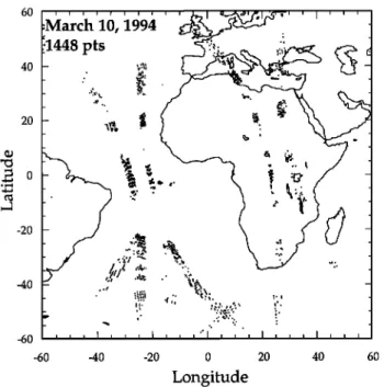
Figure 4. Location of the valid HIRS-Meteosat collocations

for a typical day. One can make out individual orbits, both ascending and descending. These orbits do not appear contin- uous because of the cloud contamination rejection.

ments are not affected by low level clouds that may be unde- tected by our simple threshold-based cloud test.

Figure 4 shows a typical example of the location of the matchups retained for 1 day. One can recognize the various polar orbiter paths, both ascending and descending. Note that

the swath of each orbit is here much narrower than the total

HIRS viewing swath because of the requirement on the view zenith angle.

4.3. Calibration Estimate

The procedure described above has been applied to 3 years

of collocated Meteosat-5 and NOAA 12 measurements. Be-

cause of the limited temporal window, some of the geostation- ary satellite images yield no valid matchups. On the other hand, when the polar satellite equatorial crossing is well within the Meteosat viewing area and the crossing time is close to the geostationary acquisition time, up to 6000 valid collocations can be derived for a single image (average is 600). Each col- location yields an estimate of the calibration coefficient:

L1

a, = CN- CN0'

(4)

where CN is the measured count, CNo is the space count (or "dark current"), L i is the radiance estimated from the HIRS 12 measurement using (3), and ai is the calibration coefficient estimate. When a sufficient number of estimates (>100) was

derived from the collocations, we set the calibration coefficient

for the image as the median value of the ai. We believe that

the median is better suited than the mean value because it is

not as affected by the few collocations that show abnormal results because of faulty data transmission, cloud detection, or sudden atmospheric change.

5. Results

Figure 5 is an example of the radiance-count scatterplot for all valid collocations during the period April 16-25, 1994. A best linear fit through the data points confirms the linearity of the instrument. The intercept yields a count of 10 for null input radiance, in close agreement with the measured space count of 8. Figure 5 confirms that the HIRS 12 and Meteosat water vapor channels yield very similar measurements. It may be compared to Figure 6 of Fan den Berg et al. [1995], where the

calculated radiance is derived from the radiosonde measure-

ments. The data points in Figure 5 show a correlation of 0.98. The equivalent correlation, reported in the description of the operational method, is of the order of 0.90, depending on the quality test used.

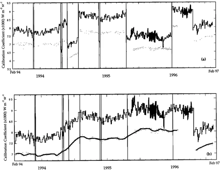
Figure 6a shows results of the procedure described in section

4 where a calibration coefficient has been derived from each

Meteosat B3 image for which more than 100 valid matchups were available. In Figure 6a we also show the operational

calibration coefficient. The results of both methods clearly

show a few sudden changes of large amplitude in the calibra- tion coefficient. These jumps correspond to a commanded change of the instrument electronic gain. The two electronic gains that have been used on Meteosat-5 yield calibration coefficients that differ by a factor of • 1.205. In order to display homogeneous results, we corrected the calibration coefficients by this factor. The periods affected by this correction are given in Table 1, and the corrected time series are shown in Figure 6b. Another sudden jump in the calibration coefficient is appar- ent in October 1996. This is not the result of a gain change. During the life of Meteosat-5, ice had diffused from other parts of the satellite and accumulated on the optics, resulting in

a loss of transmission. In order to remove this accumulation of

ice, the optics were heated, while Meteosat-6 took over the Earth monitoring. As Meteosat-5 went back on line after 5 days of interruption, the calibration coefficient had lost • 15% (increased sensitivity) and reassumed values similar to those of 1994. This indicates that the loss of sensitivity of Meteosat-5 water vapor channel with time is mostly a result of ice cover on the optics. Further evidence of the ice accumulation is pro- vided by the calibration coefficient time series. The time series show an annual cycle pattern, with a rapid increase during the

1.6 0.8 0.4 1994 Days 106-115 • q

•

Slope:

7.14

10

-3 -

, •

Correlation:O.982x,,,

• , , , ,,,,,,,,

, , , • ....

Meteosat measured count

Figure 5. Typical example of a radiance-count scatterplot for a 10-day period. The radiance is derived from the HIRS mea- surement using equation (4), whereas the count is the Meteo-

sat measurement. The line is the result of a best linear fit

BREON ET AL.: METEOSAT WATER VAPOR CHANNEL CALIBRATION 11,929 •, 9.5 , , ' I ' ' ' I , , ' I ... I ...

•'• 9 -

' 8.5

• 6.5

Figure

6. Results

of the calibration

method

described

in section

4 (dots)

together

with the operational

calibration

coefficient

(line). The vertical

lines

separate

periods

of different

gain.

Figure

6b shows

values

corrected

for the gain

factor,

using

a constant

multiplicative

value

of 1.205.

In Figure

6b the line through

the

dots shows the proposed calibration coefficient, as in Table 2.

Northern Hemisphere fall and winter (roughly October to Jan-

uary included) and a much slower decrease during the rest of

the year. This cycle

may reflect

an annual

cycle

of the Earth

mean radiative temperature, due in part to the difference of

land surfaces between the two hemispheres, that affects the

Meteosat satellite temperature.

There is clearly a large bias between the operational cali-

Table 1. Period During February 1994 to February 1997

When a Higher Gain Was Used for Meteosat Water Vapor Channel Acquisition

Begin End

Year Day Slot Year Day Slot Days 1994 146 26 1994 150 26 4 1994 299 16 1994 306 16 7 1994 335 16 1995 32 16 62 1995 144 17 1995 151 16 7 1995 297 17 1996 183 17 251

During these periods the calibration coefficients shown in Figure 6a have been multiplied by 1.205 for homogeneity with the other periods. Figure 6b and Table 2 show results obtained after this correction factor

has been applied.

bration coefficient and that retrieved by our method. The rel-

ative difference is of the order of 10-15%. Our coefficient is

lower and results in equivalent BTs roughly 3-4 K lower. Possible causes for the observed bias are discussed in section 6.

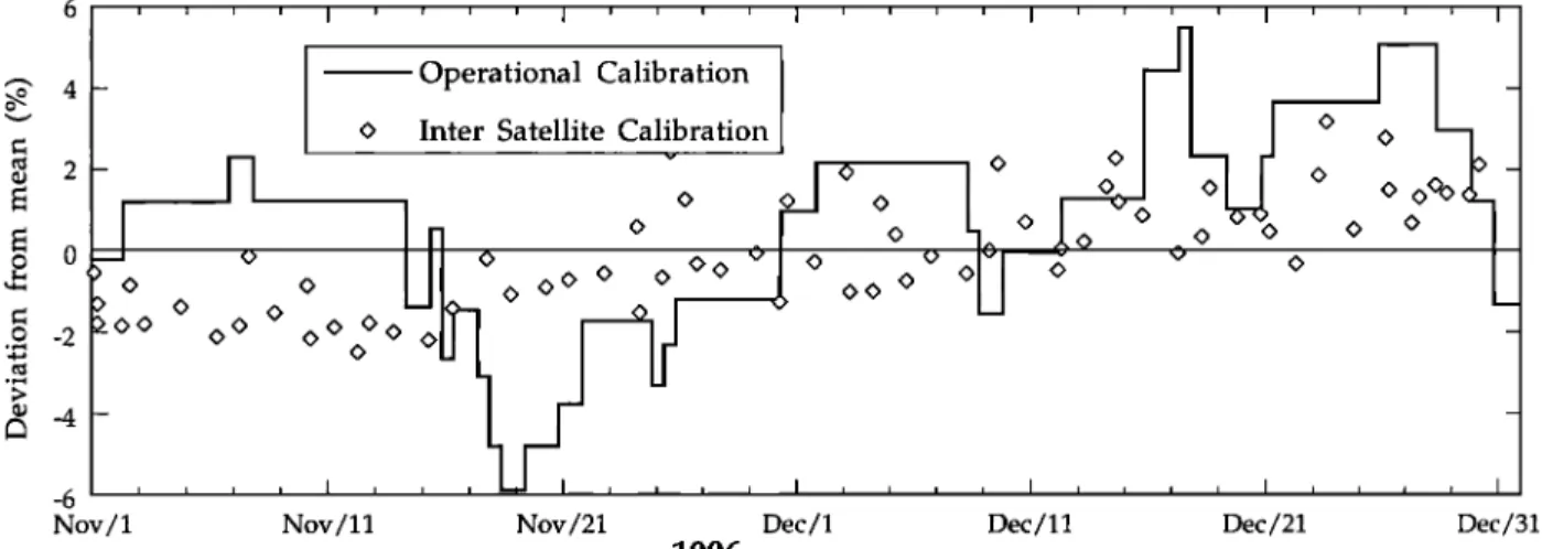
Figure 7 shows a 2-month sample of Figure 6b revealing the

temporal variability. In Figure 7 we show the deviation of the

calibration coefficient from its mean value (in %) over the

2-month period. The high-frequency variations of the calibra-

tion coefficients as measured by the two methods are uncor-

related. Similar results are obtained over all other 2-month

periods. We believe that this absence of correlation clearly

indicates that those high-frequency variations reflect the noise

inherent to each method rather than any change in the Me-

teosat radiometer sensitivity. Therefore a better estimate of

the calibration coefficient is generated by a temporal smooth-

ing of the individual estimates. This final calibration estimate is

shown in Figure 6b as a continuous line, and the numerical

values are given in Table 2 with a temporal resolution of twice

a month.

In Figure 6b, two periods, during March and September

1996, show an increased high-frequency variability in the cali-

bration coefficients. The operational calibration coefficient

11,930 BREON ET AL.' METEOSAT WATER VAPOR CHANNEL CALIBRATION o•' 4

•: o

_

•

Operational

Calibration

I

-

o Inter Satellite Calibration o o

-

[•

"

₀

0

₀

0

₀

0

_{0 O0}

_

J

0

0

0 OO•:•-O

0 0 0

> 0

0

_ 0 O0 0 0

0

• o o

•[]J

--

•_oo o o oOgo

_

Nov / 11 Nov/21 Dec / 1 Dec / 11 Dec/21 Dec/31

1996

Figure 7. Subset of Figure 6b with higher temporal resolution. The figure shows the deviation of the calibration coefficient from its mean value over the 2-month period considered here (November-December 1996).

day. These periods correspond to the equinoxes when Meteo- sat is in the Earth shadow around midnight. Therefore the images used for the calibration using the 0000 UT radiosondes may be acquired from a satellite colder than during normal operation. This would explain the diurnal variability of the calibration coefficient. It is not clear, however, why this feature is not apparent in 1994 and 1995.

6. Discussion

6.1. Calibration of HIRS 12

A critical point for the accuracy of the method is the cali-

bration of the HIRS 12 measurements. This calibration is

achieved on board, using cold and warm targets of known temperatures. An independent evaluation may be obtained from in situ measurements with a procedure similar to the operational calibration of Meteosat water vapor channel. Ra- diative transfer calculations applied to radiosondes have been compared to collocated HIRS 12 measurements [i.e., Soden and Lanzante, 1996]. Such comparisons have shown large dif- ferences that were generally attributed to biases in the mea- surement of humidity by radiosondes. Soden and Lanzante [1996] show that the sign and magnitude of these biases are dependent on the humidity sensor used on the radiosonde. Therefore it is difficult to distinguish from such comparisons a bias in the radiometer calibration from biases introduced by the humidity measurement.

On the other hand, the onboard calibration procedure for

the HIRS 12 is the same for all HIRS channels. Therefore it is

legitimate to assume that the accuracy of this calibration is similar for all channels. The midtroposphere temperature channels (5, 6, and 15) provide the most meaningful evaluation because of the accuracy of the corresponding in situ measure- ment. Comparisons of measured and simulated brightness temperatures for these channels show agreements better than I K [Susskind et al., 1983; Murty et al., 1993]. These errors also

include collocation and radiative transfer calculation errors.

Thus we believe that the accuracy of the HIRS 12 calibration

is better than I K.

6.2. Accuracy of the Method

Other sources of uncertainty in the method are collocation errors, cloud contamination, radiative transfer modeling, and

uncertainties in the filter spectral responses. We believe that

the collocation and the cloud contamination result in unbiased

errors. The magnitude of the random errors may be evaluated from the scatter around the best linear fit in Figure 5. Figure 8 shows a histogram of the deviation of individual slopes which can be derived from each collocation as in (4). This histogram

shows that random errors in the method for individual collo-

cations is of the order of 3.5%. Moreover, its shape indicates that the error distribution is roughly Gaussian, so that a large error reduction is expected when taking the median value of the distribution. Note, however, that, for a given Meteosat image, the valid collocations may be within a rather small area, with specific atmospheric conditions, so that the statistic may not lead to a cancellation of errors as expected from a pure random process. The time series (Figures 6 and 7) indicate, nevertheless, that the random error on the image calibration estimates, when using > 100 collocation results, is of the order

of 1%.

More worrisome is the potential impact of the radiometer spectral response on the results. Clearly, if one (or both) of the spectral responses differs significantly from those used here (and in other studies), it would have an impact on (3) and may lead to a bias in the results. Br•on et al. [1999] shows that the spectral response of the GMS water vapor channel is contam- inated by atmospheric absorption during the measurement. Although no such feature is apparent on the spectral responses

used here, it cannot be ruled out.

Radiative transfer modeling is also a possible cause for bias. The MODTRAN model is used to derive (3). However, be- cause our method compares the measurement of two similar channels, errors in the radiative transfer modeling are likely to

cancel out. On the other hand, an error in the radiative transfer

modeling may have a larger impact on the operational method results. This point is further discussed in section 6.4.

6.3. High-Frequency Variability

Figure 7 as well as similar figures for other 2-month periods (not shown) show that the variability of the inter satellite calibration coefficient is of the order of 1%, after the long-term drift has been removed. This result clearly demonstrates that the stability of both instruments on short timescales is better than this estimate. An exception to this rule may be observed for a few images just after midnight during the equinox peri-

BREON ET AL.' METEOSAT WATER VAPOR CHANNEL CALIBRATION 11,931

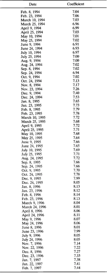
Table 2. Proposed Calibration Coefficient for Meteosat-5

Derived From the Intercalibration With NOAA 12/HIRS 12

Date Coefficient Feb. 8, 1994 7.04 Feb. 23, 1994 7.06 March 10, 1994 7.03 March 25, 1994 6.96 April 9, 1994 6.99 April 25, 1994 7.03 May 10, 1994 7.01 May 25, 1994 7.02 June 9, 1994 6.91 June 24, 1994 6.93 July 10, 1994 6.97 July 25, 1994 7.00 Aug. 9, 1994 7.00 Aug. 24, 1994 7.02 Sep. 8, 1994 7.02 Sep. 24, 1994 6.94 Oct. 9, 1994 7.02 Oct. 24, 1994 7.13 Nov. 8, 1994 7.17 Nov. 23, 1994 7.26 Dec. 9, 1994 7.40 Dec. 24, 1994 7.53 Jan. 8, 1995 7.65 Jan. 23, 1995 7.73 Feb. 8, 1995 7.79 Feb. 23, 1995 7.78 March 10, 1995 7.72 March 25, 1995 7.68 April 9, 1995 7.72 April 25, 1995 7.71 May 10, 1995 7.68 May 25, 1995 7.64 June 9, 1995 7.66 June 24, 1995 7.65 July 10, 1995 7.69 July 25, 1995 7.71 Aug. 24, 1995 7.72 Sep. 8, 1995 7.66 Sep. 24, 1995 7.66 Oct. 9, 1995 7.70 Oct. 24, 1995 7.78 Dec. 9, 1995 7.99 Dec. 24, 1995 8.05 Jan. 8, 1996 8.13 Jan. 23, 1996 8.12 Feb. 8, 1996 8.14 Feb. 23, 1996 8.13 March 9, 1996 8.04 March 24, 1996 8.01 April 8, 1996 8.06 April 24, 1996 8.11 May 9, 1996 8.07 May 24, 1996 8.06 June 8, 1996 8.01 June 23, 1996 7.99 July 9, 1996 8.05 July 24, 1996 15.05 Nov. 7, 1996 7.14 Nov. 22, 1996 7.22 Dec. 8, 1996 7.27 Dec. 23, 1996 7.33 Jan. 7, 1997 7.38 Jan. 22, 1997 7.41 Feb. 7, 1997 7.44

The temporal resolution is 24 points per year.

ods. When Meteosat goes into and goes out of the Earth

shadow, the satellite goes into a rapid temperature change

which affects its calibration. The corresponding images should

be avoided for quantitative studies.

8OO 700

z• 600

• 500

• 200

Figure 8. Histogram of the deviation from the slope ex-

pressed in percent for individual collocations. This figure is

based on the collocations acquired during April 16-25, 1994, shown in Figure 5.

The operational calibration coefficient shows variability of

the order of 5% and up to 10% on short timescales (1 day to

2 weeks), not limited to the eclipse periods, which do not

appear on our results. This result indicates that these varia-

tions do not reflect a change in the instrument, but are rather a result of the statistical noise in the operational calibration

method.

6.4. Bias

Figure 6 shows that the operational calibration method and

the calibration derived from the HIRS instrument yield rather

different results. The observed differences in the calibration

coefficient are of the order of 10-15%. Such differences yield

a brightness temperature bias of the order of 3-4 K. For water

vapor studies, these differences are equivalent to a relative bias

of 35-50% on the Upper Tropospheric Humidity (UTH).

Clearly, such differences cannot be ignored.

The operational calibration coefficients are derived from

radiosonde measurements. The humidity measurements pro-

vided by such devices are known to be subject to large errors,

in particular for dry and/or cold conditions [Wade, 1994; Larsen

et al., 1993]. Soden and Lanzante [1996] analyze collocations of

radiosondes and HIRS channel 12 measurements. Top of the

atmosphere radiances are calculated using the radiosonde pro-

files and compared to the satellite measurements. Significant

biases are found, the sign of which depends on the type of

humidity sensors used. This study clearly demonstrates that

there may be a large bias in the measurement of UTH by

radiosondes. Within the field of view of Meteosat at 0 ø longi-

tude over the equator, most radiosondes carry carbon hygristor

or capactitive humidity sensors. For these types of sensors,

1_2 •-_ •-1•

Soden and Lanzante [1996] find a warm mas computed tu mc

satellite measurement. The bias magnitude is "roughly 3-4 K,"

in complete agreement with the present study results. Note,

however, that the authors suspect a bias in their radiative

transfer modeling which may explain half of the bias, as con-

firmed by recent radiative transfer model intercomparisons

[Soden et al., 2000].

The operational procedure extrapolates the humidity mea-

surement above 300 hPa. Figure 1 shows that the transmission

between the 300 hPa level and the top of the atmosphere is far from unity. This result indicates that the Meteosat water vapor

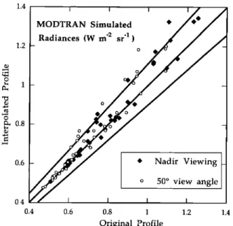
11,932 BREON ET AL.: METEOSAT WATER VAPOR CHANNEL CALIBRATION 1.4 1.2 0.6 0.4 0.4 0.6 0.8 1 1.2 1.4 Original Profile

Figure 9. Effect of the linear extrapolation of relative hu- midity on the top of the atmosphere radiance for the Meteosat water vapor channel. Radiances are calculated with MOOT- RAN for atmospheric profiles where the relative humidity has been extrapolated above 300 hPa as in the operational calibra- tion method as a function of those obtained with the original profiles. The lines indicate a perfect agreement as well as 10%

deviations.

channel is quite sensitive to the atmospheric conditions above that level. Therefore the humidity extrapolation may also yield

a bias.

We conducted a sensitivity study using 42 atmospheric pro- files carefully prepared for their consistent humidity values in the upper troposphere [Soden et al., 2000]. For these profiles we computed the top of atmosphere radiance for the Meteosat spectral response using the original water vapor profile and that extrapolated as in the operational calibration procedure. Results are shown in Figure 9. The computed radiances are very similar for about half of the profiles. On the other hand, the other half show a systematic larger radiance for the inter- polated profiles, up to > 10%, consistent with the fact that they are drier than the originals above 300 hPa. This difference may explain the bias between the operational calibration and that derived from our method. The atmospheric profiles probed by

Meteosat over the radiosonde stations used for the calibration

may or may not be similar to profiles with the 10% difference. Therefore, at this point, one cannot quantify the bias gener- ated by the extrapolation procedure within the 0-10% range. However, the hypothesis of a large bias, consistent with the

difference between the two method results, cannot be ruled out. Another concern is the radiative transfer modeling used to

calculate top of atmosphere radiance from the radiosonde profiles. Soden et al. [2000] show that most models yield con- sistent results in the spectral range of interest. Their study includes both line-by-line and band models. However, this agreement is not a proof of the model accuracy. The opera-

tional calibration method is much more sensitive than our

method to errors in the radiative transfer modeling, and such errors may explain the difference in the results.

Most quantitative applications of the Meteosat water vapor

channel make use of a radiative transfer model consistent with

that used in the operational calibration method. Therefore a bias in the radiative transfer modeling would mostly cancel out when using an assumed biased operational calibration coeffi- cient for a geophysical application.

6.5. Implications for iSCCP Data

We believe that the present study demonstrates that the operational calibration coefficient (i.e., nominal) of the Me- teosat water vapor channel can be improved using an intersat-

ellite calibration. The short-term variations cannot be attrib-

uted to the radiometer, and there are systematic differences with our method results. A large fraction of Meteosat data used for climate study purposes are distributed in the B3 for- mat, which includes other calibration tables (see section 4.1).

Therefore it is legitimate to wonder if these calibration tables

can be used instead. The "normalized" and "absolute" calibra-

tion tables are derived, as in the present study, from colloca- tions between HIRS 12 and the geostationary satellites. The main difference, however, is that the objective is to mimic HIRS 12. Our method attempts to reproduce the bias between HIRS 12 and the Meteosat water vapor channels that is ob- served on the simulations (see Figure 2). The products of the calibration method are two coefficients, slope and intercept,

derived from a linear best fit between the two satellite BTs.

These coefficients are used to correct the operational bright- ness temperature calibration tables. They are computed with a period of 1 month, although a higher frequency is possible.

Therefore the normalized and absolute calibration tables re-

produce the short-term variability of the operational calibra- tion. This variability should be corrected.

7. Conclusions

We propose an alternative method for the operational cal- ibration of Meteosat water vapor channel. This method has been applied to 3 years of Meteosat-5 data. Our results show a significantly smaller short-term variability than the operational calibration, indicating that the instrument is more stable than suggested by the nominal calibration. Moreover, the results indicate that the operational calibration coefficient is 10-15% too large. We propose three likely hypotheses for the bias

between the two method results:

1. The measurement of upper tropospheric water vapor by radiosondes may be biased.

2. The extrapolation of humidity measurements above 300 hPa in the operational calibration procedure may yield a bias for atmospheric conditions prevailing over the selected stations.

3. The radiative transfer modeling in the spectral range of interest may yield biased results.

In geophysical applications that use explicitly or implicitly a

radiative transfer model to invert the satellite measurements,

biases in the calibration coefficients and in the inversion pro- cedure that result from modeling errors may mostly cancel out. If so, it is better to use calibration coefficients in the range of the operational coefficients, although the high-frequency vari-

ations must be corrected. On the other hand, if one of the two

first hypotheses is correct, it is better to use the coefficient proposed in Table 2. The use of the operational calibration coefficient, corrected for the short-term variability, would lead to geophysical products consistent with radiosonde measure- ments. The use of the calibration coefficients proposed in this paper would lead to products consistent with those derived

BREON ET AL.: METEOSAT WATER VAPOR CHANNEL CALIBRATION 11,933

Acknowledgments. The Meteosat data used in this paper were obtained from the NASA Langley Research Center, EOSDIS Distrib-

uted Archive Center. Thanks are due to Stephen Tjemkes for con- structive criticisms on an earlier version of the manuscript and to two

anonymous reviewers for editorial corrections.

References

Beriot, N., N. A. Scott, A. Chddin, and P. Sitbon, Calibration of

geostationary-satellite infrared radiometers using the TIROS-N ver-

tical sounder: Application to METEOSAT-1, J. Appl. Meteorol., 21, 84-89, 1982.

contamination on the measurement of the spectral response of GMS-5 water vapor channel, J. Atmos. Oceanic Technol., 16, 1851-

1853, 1999.

Chaboureau, J.-P., A. Chfdin, and N. A. Scott, Remote Sensing of the vertical distribution of atmospheric water vapor from the TOVS obse•ations: Method and validation, J. Geophys. Res., 103, 8743- 8752, 1998.

Ch6din, A., Improved initialization inversion method: A high- resolution physical method for temperature retrievals from satellites of the TIROS-N series, J. Clim. Appl. Meteorol., 24, 128-143, 1985. Desormeaux, Y., W. B. Rossow, C. L. Brest, and G. G. Campbell,

Normalisation and calibration of geostationa• satellite radiances

for ISCCP, J. Atmos. Ocean. Technol., 10, 304-325, 1993. Larsen, J. C., E. W. Chiou, W. P. Chu, M.P. McCormick, L. R.

McMaster, S. Oltmans, and D. Rind, A comparison of the Strato-

spheric Aerosol and Gas Experiment II tropospheric water vapor to

radiosonde measurements, J. Geophys. Res., 98, 4897-4917, 1993. Murty, D. G. K., W. L. Smith, H. M. Woolf, and C. M. Hayden,

Comparison of radiances obse•ed from satellite and aircraft with calculations by using •o atmospheric transmittance models, Appl.

Opt., 32(9), 1620-1628, 1993.

Roca, R., L. Picon, M. Desbois, H. LeTreut, and J.-J. Morcrette,

Direct comparison of METEOSAT water vapor channel data and

general circulation model results, Geophys. Res. Lett., 24, 147-150,

1997.

Schiffer, R. A., and W. B. Rossow, ISCCP global radiance dataset: A

new resource for climate research, Bull. Am. Meteorol. Soc., 66, 1498-1505, 1985.

Schmetz, J., W. P. Menzel, C. Veldon, X. Wu, L. Van den Berg, S. Nieman, C. Hayden, K. Holmlund, and C. Geijo, Monthly mean large-scale analysis of upper-tropospheric humidity and wind field

divergence derived from three geostationary satellites, Bull. Am. Meteorol. Soc., 76, 1578-1584, 1995.

Soden, B. J., and J. R. Lanzante, An assessment of satellite and radiosonde climatologies of upper-tropospheric water vapor,

J. Clim., 9, 1235-1250, 1996.

Soden, A., et al., An intercomparison of radiation codes for retrieving

upper tropospheric humidity in the 6.3 micron band: A report from the first Gvap workshop, Bull. Am. Meteorol. Soc., in press, 2000.

Susskind, J., J. Rosenfield, and D. Reuter, An accurate radiative trans- fer model for use in the direct physical inversion of HIRS-2 and

MSU temperature sounding data, J. Geophys. Res., 88(C13), 8550- 8568, 1983.

Van den Berg, L. C. J., A. Pyomjamsri, and J. Schmetz, Monthly mean upper tropospheric humidities in cloud-free areas from METEO- SAT observations, Int. J. Climatol., 11, 819-826, 1991.

Van den Berg, L. C. J., J. Schmetz, and J. Whitlock, On the calibration of the Meteosat water vapor channel, J. Geophys. Res., 100, 21,069-

21,076, 1995.

Wade, C. G., An evaluation of problems affecting the measurement of low relative humidity on the United States radiosonde, J. Atmos.

Oceanic Technol., 11, 687-700, 1994.

Wang, J., G. P. Anderson, H. E. Revercomb, and R. O. Knuteson,

Validation of FASCOD3 and MODTRAN3: Comparison of model

calculations with ground-based and airborne interferometer obser- vations under clear-sky conditions, Appl. Opt., 35, 6028-6040, 1996. J. J. Bates, Climate Diagnostic Center, NOAA/ERL/CDC, 325

Broadway, Boulder, CO 80303. (jbates@etl.noaa.gov)

F.-M. Brdon, Laboratoire des Sciences du Climat et de

l'Environnement, CEA/DSM, 91191 Gif sur Yvette Cedex, Saclay,

France. (fmbreon@cea.fr)

D. L. Jackson, Climate Diagnostic Center, Cooperative Institute for Research in Environmental Sciences, University of Colorado, Boulder,

CO 80302.

(Received August 18, 1999; revised December 6, 1999; accepted December 17, 1999.)