Sound, Complete, and Tractable Linearizability Monitoring for Concurrent Collections

HAL Id: hal-01943932

https://hal.archives-ouvertes.fr/hal-01943932

Submitted on 4 Dec 2018

HAL is a multi-disciplinary open access

archive for the deposit and dissemination of

sci-entific research documents, whether they are

pub-lished or not. The documents may come from

teaching and research institutions in France or

abroad, or from public or private research centers.

L’archive ouverte pluridisciplinaire HAL, est

destinée au dépôt et à la diffusion de documents

scientifiques de niveau recherche, publiés ou non,

émanant des établissements d’enseignement et de

recherche français ou étrangers, des laboratoires

publics ou privés.

Monitoring for Concurrent Collections

Michael Emmi, Constantin Enea

To cite this version:

Michael Emmi, Constantin Enea. Sound, Complete, and Tractable Linearizability Monitoring for

Concurrent Collections. Proceedings of the ACM on Programming Languages, ACM, 2017.

�hal-01943932�

Sound, Complete, and Tractable Linearizability Monitoring

for Concurrent Collections

MICHAEL EMMI,

CONSTANTIN ENEA,

While many program properties like the validity of assertions and in-bounds array accesses admit nearly-trivial monitoring algorithms, the standard correctness criterion for concurrent data structures does not. Given an implementation of an arbitrary abstract data type, checking whether the operations invoked in one single concurrent execution are linearizable, i.e., indistinguishable from an execution where the same operations are invoked atomically, requires exponential time in the number of operations.

In this work we identify a class of collection abstract data types which admit polynomial-time linearizability monitors. Collections capture the majority of concurrent data structures available in practice, including stacks, queues, sets, and maps. Although monitoring executions of arbitrary abstract data types requires enumerating exponentially-many possible linearizations, collections enjoy combinatorial properties which avoid the enumeration. We leverage these properties to reduce linearizability to Horn satisfiability. As far as we know, ours is the first sound, complete, and tractable algorithm for monitoring linearizability for types beyond single-value registers.

CCS Concepts: • Software and its engineering → Formal software verification; • Theory of computa-tion → Logic and verificacomputa-tion; • Computing methodologies → Concurrent algorithms;

Additional Key Words and Phrases: Linearizability; Runtime Verification; Concurrent Objects ACM Reference Format:

Michael Emmi and Constantin Enea. 2018. Sound, Complete, and Tractable Linearizability Monitoring for Concurrent Collections. Proc. ACM Program. Lang. 2, POPL, Article 25 (January 2018),27pages.https://doi. org/10.1145/3158113

1 INTRODUCTION

Efficient multithreaded programs typically rely on optimized implementations of common abstract data types (adts) like stacks, queues, sets, and maps [Liskov and Zilles 1974], whose operations exe-cute in parallel across processor cores to maximize efficiency [Moir and Shavit 2004]. Programming these “concurrent data structures” is tricky though. Synchronization between operations must be minimized to reduce response time and increase throughput [Herlihy and Shavit 2008;Moir and Shavit 2004]. Yet this minimal amount of synchronization must also be adequate to ensure that operations behave as if they were executed atomically, one after the other, so that client programs can rely on their (sequential) adt specification; this de-facto correctness criterion is known as linearizability [Herlihy and Wing 1990]. These opposing requirements, along with the general challenge in reasoning about thread interleavings, make concurrent data structures a ripe source of insidious programming errors [Michael 2004].

Authors’ addresses: Michael Emmi, SRI International, USA, michael.emmi@sri.com; Constantin Enea, IRIF, Univ. Paris Diderot & CNRS, France, cenea@irif.fr.

Permission to make digital or hard copies of part or all of this work for personal or classroom use is granted without fee provided that copies are not made or distributed for profit or commercial advantage and that copies bear this notice and the full citation on the first page. Copyrights for third-party components of this work must be honored. For all other uses, contact the owner/author(s).

© 2018 Copyright held by the owner/author(s). 2475-1421/2018/1-ART25

Program properties like linearizability that are difficult to determine statically are typically substantiated by dynamic techniques like testing and runtime verification. Besides increasing confidence in the validity of such properties, property monitoring enables the eager diagnosis of anomalies which may otherwise only exhibit far-removed manifestations. However, while typical safety properties like the validity of assertions and in-bound array accesses admit nearly-trivial monitors which require only linear time in the length of program executions [Havelund and Rosu 2004], monitoring linearizability of an execution against an arbitrary adt specification requires exponential time [Gibbons and Korach 1997]. This lower-bound limits precise monitoring to very short executions with few operations [Burckhardt et al. 2010], ultimately rendering testing and runtime verification ineffective for concurrent data structures, and limiting practical utilization to a small number of trusted implementations.

In this work we identify a class of adts, called collection types, which admit polynomial-time linearizability monitors. Intuitively, collection types capture the typical collection-based data struc-tures, including the stacks, queues, sets, and maps provided by libraries like java.util.concurrent. Technically, we characterize collection types as containers of values whose operations add, remove, and use values. In addition, collection types satisfy four semantic properties: value invariance excludes types whose operations have effects beyond adding and removing values; locality ex-cludes types whose operations add or use values beyond those appearing as arguments or returns; parametricity excludes types whose operations use values un-opaquely; reducibility excludes types which are not fully characterized by small representative behaviors. While in practice concurrent data structures often provide auxiliary operations which are not value invariant, local, or reducible, such methods often eschew linearizability in the name of efficiency. For example, while the size method of a collection adt is typically neither local nor reducible, it is also not typically linearizable because the cost of synchronization required for atomically tallying, or maintaining a tally of, all elements apparently outweighs the need for a precise count. Recent work demonstrates that the majority of these auxiliary methods are not linearizable [Emmi and Enea 2017], and thus our focus on ensuring linearizability for value-invariant, local, parametric, and reducible methods of a collection adt may not amount to a significant practical restriction.

The challenge we face in demonstrating tractability of the linearizability problem for collection types is avoiding an exponential enumeration. Since the operations of a concurrent data structure are permitted to execute in parallel, the happens-before order among the operations of any given execution is generally only a partial linearization, i.e., a partial order. This partial linearization is consistent with a given adt when it can be extended to a total linearization whose resulting sequence of operations is admitted. However, there are generally an exponential number of total extensions to a given partial linearization, and for an arbitrary adt, enumerating each extension is asymptotically optimal [Gibbons and Korach 1997].

Our result establishes that the exponential enumeration of total linearizations is avoidable for collection types. Our proof is essentially by reduction to a logical satisfiability problem in which models represent linearizations, and formulas encode linearization constraints, including an axiomatization of total orders to ensure that the resulting linearization is total. The input to this satisfiability problem is an operation-order specification (oos) which amounts to an encoding of the constraints of a given adt as a conjunction of Horn clauses, i.e., of disjunctions with at most one positive literal. Unlike formulas with arbitrary propositional structure, satisfiability of conjunctions of Horn clauses is tractable [Dowling and Gallier 1984]. Intuitively, Horn satisfiability avoids the exponential enumeration of possible satisfying assignments, corresponding to the exponential enumeration of total linearizations. However, the totality axioms require clauses like x = y ∨ x < y ∨ y < x which are not Horn. The crux of our result lies in the Hornification of

formulas which include total-order axiomatization: they can be rewritten to equisatisfiable Horn formulas.

The reduction to this tractable logical satisfiability problem — called oos linearizability — is another challenge. Essentially, we must show that the semantic properties which define collection types guarantee the existence of sound operation-order specifications, so that oos linearizability is equivalent to linearizability.

We fulfill this reduction by showing that the locality and parametricity properties ensure a nice combinatorial property: when arbitrarily-large operation sequences embed, in a certain precise sense, subsequences which are violations, i.e., are not admitted by the collection type, the larger sequences are themselves violations. Furthermore, the value-invariance and reducibility properties ensure that there are a finite number of minimal violations, which can thus be thought of as the atomic patterns which every violation embeds, and that these patterns are bounded in size. Collectively, these combinatorial properties ensure that collection types have sound operation-order specifications, with constraints corresponding to the exclusion of violation patterns.

To the best of our knowledge, our result yields the first tractable, sound, and complete algorithm for checking linearizability for collection adts, representing the majority of practically-available concurrent data structures. Our work is complimented by others which demonstrate effective implementations of inference [Emmi and Enea 2016] and runtime monitoring [Emmi et al. 2015] of operation-order specifications. In particular [Emmi et al. 2015] evaluated the performance of an implementation of the algorithm we prove sound, demonstrating orders of magnitude improvement in runtime verification. While these works conjectured their soundness (i.e., the guarantee that every linearizability violation is identified) based on empirical evidence, our result amounts to the first conclusive proof of their soundness.

Our contributions and outline are summarized as follows:

§3 identifies the class of collection types, demonstrates naturally-occurring instances like stacks, queues, sets, and maps, and states our main result on polynomial-time linearizability moni-toring.

§4 reduces linearizability to a logical satisfiability problem requiring sound operation-order specifications.

§5 proves that linearizability against operation-order specifications is tractable, by reduction to Horn satisfiability.

§6 demonstrates key combinatorial properties of collection types enabling characterization via violation patterns.

§7 demonstrates that sound operation-order specifications are guaranteed to exist for collection types.

Section2recalls the linearizability problem and its intractability, Sections8and9conclude with a discussion of related work and concluding remarks.

2 LINEARIZABILITY

Efficient implementations of concurrent software components use fine-grain atomic operations to allow their methods to execute concurrently [Herlihy and Shavit 2008]. Reasoning about the correctness of such implementations thus requires specifying the expected behavior of concurrently-executed methods. Typical specification mechanisms for sequentially-concurrently-executed methods describe the pre- and post-conditions of methods executed in isolation [Hoare 1969]. To reduce the mean-ings of concurrent behaviors to those of sequential behaviors, linearizability [Herlihy and Wing 1990] demands that some linearization of the only partially-ordered observed concurrent method

invocations must correspond to a valid sequential behavior. In this section we formalize notions of behavior and specification which define the linarizability problem addressed in the remainder.

Accordingly, an invocation labelm(®v) is a method name m along with a vector ®v of argument values. An operation label ℓ= m(®v) ⇒ v is an invocation label m(®v) along with a return value v. We write args(ℓ) to denote the multiset of argument valuesÒ

ivi, and vals(ℓ) to denote the multiset

of argument and return values args(ℓ) ∪ {v}. An interface is a set of operation labels over a finite set of method names. In this work we consider only fixed-arity interfaces, i.e., the number of method arguments is fixed, where argument and return values have opaque infinite-domain polymorphic types, i.e., which can be instantiated with arbitrary datatypes including integers, strings, and object references.

Remark 2.1. While our simplified formalization allows only argument and return values from infinite domains, our results are easily extended to consider values from any finite domain as well, e.g., Boolean values, e.g., null values. There is no loss of generality in supposing method names include such finite-domain return values since we consider completed operations only. For instance, a set type would include operations void-type operations containsTrue(v) and containsFalse(v) in place of Boolean operations contains(v) ⇒ b.

Definition 2.2. An abstract data type (adt) is a prefix-closed set of operation-label sequences over a fixed-arity interface.

Example 2.3. The stack type is the set of sequences of push(v) and pop ⇒ v operations including push(1) · push(2) · pop ⇒ 2 · pop ⇒ 1 and

push(1) · pop ⇒ 1 · push(2) · pop ⇒ 2

in which the response of each pop operation matches the most-recent unmatched push operation’s argument. Queues with enqueue(v) and dequeue ⇒ v operations are described similarly. Following Remark2.1, the set type includes the operations addTrue(v), removeTrue(v), containsTrue(v), and their counterparts, addFalse(v), etc.

Example 2.4. The key-value map type includes put(k,v) ⇒ b operations, binding the key k to valuev and returning a Boolean b indicating whether a binding of key k is overwritten, along with remove(k) ⇒ v operations, removing and returning a possibly-null (see Remark2.1) valuev bound to keyk, and get(k) ⇒ v operations, returning the possibly-null value v bound to key k.

A history ⟨O, ≺⟩ is a function O mapping operations to operation labels, along with a happens-before partial-order ≺ over the operations dom(O). A linearization of a history h is a sequence s of operation labels such that:

• s and h have the same labels: s_i = O(f (i)), and • s preserves the order of h: i < j if f (i) ≺ f (j),

for some bijectionf : | dom(O)| → dom(O) between indices and operations. In the worst case there are O(kn_{) linearizations of a history withn operations of which at most k are mutually unordered.}

Definition 2.5. The linearizability problem asks whether a given adt includes some linearization of a given history.

Example 2.6. The history with concurrent operations push(1) and push(2) preceding pop ⇒ 1 is linearizable since the stack type admits the linearization push(2) · push(1) · pop ⇒ 1. The history would not be linearizable were push(1) to precede push(2), since the stack type does not admit its only possible linearization, push(1) · push(2) · pop ⇒ 1.

Adept readers may notice that our definition assumes all operations are completed. This is for technical convenience only. The linearizability problem remains np-hard even when all operations are completed, and the forthcoming tractability results of our work hold for an arbitrary number of concurrent operations, so long as the number of non-read-only pending operations at the time of a linearizability check is bounded.

Theorem 2.7. The linearizability problem is np-complete.

Proof. SeeGibbons and Korach[1997]. □ While this work is devoted to the analysis of individual histories, one can also consider the analysis of adt implementations. An implementation is essentially a transition system with call actions, corresponding to method invocations from client programs, and return actions, corresponding to method returns. Each execution corresponds to a single history in which each pair of operations is ordered if the first’s return occurs before second’s invocation. The set of all possible executions over all possible clients thus yields a set of histories associated with an implementation. Taking an abstract view, we say an implementation of an adt is a set of histories, and that the implementation is linearizable if all of its histories are linearizable according to the adt. We leverage this concept in Section4to form a notion of soundness of our approach to linearizability checking of individual histories.

3 COLLECTION TYPES

In this section we identify a class of collection abstract data types which admit polynomial-time linearizability monitors. We characterize this class with a semantic notion of the state of an arbitrary type as a container of values. This notion of state gives rise to other semantic notions, such as whether a given operation adds a given value to the state or uses a given value from the state. We build from these semantic notions the four properties that define collections: value invariance, locality, parametricity, reducibility. Finally, we conclude the section by stating our main result.

We begin by developing a notion of observation-based states. An observation from a sequence s ∈ T of an abstract data type T is an operation-label sequence s′_{such thats ·s}′_{∈T . Two sequences}

s, s′ _{∈T are distinguishable by an observation s}′′_{whens · s}′′ _{∈T and s}′_·s′′

< T or vice versa. Two sequencess, s′_{∈T are equivalent, written s ≡ s}′_{, when they are not distinguishable by any}

observation.

Example 3.1. Consider the following stack behaviors: push(1) · push(2),

push(3) · push(2), and

push(1) · push(2) · push(3) · pop ⇒ 3.

While the first two sequences are distinguishable by the observation pop ⇒ 2 · pop ⇒ 1, the first and third sequences are equivalent.

We represent states with canonical representatives of equivalence classes of observations. Given any total order ≪ on operation labels, e.g., lexicographic order over method names and argument and return valuesm· ®v ·v, we lift ≪ to operation-label sequences, ordering equal-length sequences by lexicographic order, and ordering unequal-length sequences by their length; i.e.,s ≪ s′_{iff |s| < |s}′_|

or |s| = |s′_{| and there existsi for which s}

i ≪si′andsj = s′jfor allj < i. The state, or construction

sequence,Js K of an operation-label sequence s is the minimum equivalent operation-label sequence: Js K = min_≪ {s

′

readonly(s · ℓ) ⇔Js · ℓK = Js K

adds(s · ℓ,v) ⇔ v ∈ (contents(s · ℓ) \ contents(s)) removes(s · ℓ,v) ⇔ v ∈ (contents(s) \ contents(s · ℓ))

uses(s · ℓ,v) ⇔ drop(s, {v}) · ℓ < T

touches(s · ℓ,v) ⇔ adds(s · ℓ,v) ∨ uses(s · ℓ,v)

Fig. 1. Operation predicate semantics.

Thus we represent the state after a given operation sequence as the minimal sequence which yields the same observations.

We associate each sequence with a multiset of values that its state contains: those which occur as arguments in the minimum equivalent sequence. We write args(s) to denote the multiset Òiargs(ℓi)

of argument values in the sequences = ℓ0ℓ1. . .; the contents of a sequence s is the multiset

contents(s) = args(Js K) of arguments to the construction sequence Js K. Intuitively, the argument values ofJs K define the values contained after executing s ; the responses of subsequent method invocations would not include any removed valuev, and thus the state, being a minimal sequence, would not contain operations addingv.

Example 3.2. The following stack behaviors push(2),

push(1) · pop ⇒ 1 · push(2), and

push(1) · pop ⇒ 1 · push(2) · push(3) · pop ⇒ 3 all have the same state, push(2).

We define the class of collection types as properties on operation sequences. An operation predicate is a predicateP(s, ®v) on non-empty operation-label sequences s = s′_{·ℓ and values ®v}

denoting a property of the operation labeled ℓ from the context of the operation-label sequences′_.

The occurrences of an operation predicateP in operation-label sequence s over value vector ®v is the set

P∗_{(s, ®v) = {i : P(s}

0· · ·si, ®v)}

of operation indices at whichP holds.

Figure1lists the semantics of several operation predicates. We write drop(s,V ) to denote the

maximal subsequences′ofs such that vals(s′)∩V = ∅, where vals(s) denotes the multiset Ò_ivals(ℓi) of argument and return values in the sequences = ℓ0ℓ1. . .. We treat unary operation predicates as

adjectives, e.g., saying an operation is “read-only,” and binary predicates as verbs, e.g., saying an operation “adds” a given value. An operation labeled ℓ following a sequences is read-only when it leaves the construction sequence unchanged; the operation adds or removes a valuev when the difference in contents before and after includesv; the operation uses v when its response is invalid werev not present; finally, the operation touches v when it either adds v or uses v.

Example 3.3. The push(v) operations of the stack type add v, while the pop ⇒ v operations remove and usev. A peek ⇒ v operation, returning the most-recently pushed value v, would be read-only and usev.

The first property of collection types excludes operations which have any affect besides adding or removing values. Technically, a type is value invariant when each operation which uses a value v either removes v or is read-only.

Example 3.4. The stack type with push, pop, and peek operations is value invariant. A stack type which supported an operation that increments the most-recently pushed (integer) value would not be value invariant. Similarly, the queue, set, and map types in Examples2.3–2.4are value invariant.

The second property of collection types excludes operations which touch values that do not appear as argument or return values. Technically, a local interpretation for an operation predicateP and abstract data typeT is a predicate P′_{on individual operation labels such that for all sequences}

s · ℓ ∈ T we have P(s · ℓ, ®v) iff P′_{(ℓ, ®v). We say that a type is local when local interpretations exist}

for the readonly, adds, and uses predicates1_{of Figure1, and its operations touch exactly the values}

appearing in its label, i.e.,v ∈ vals(ℓ) ⇔ touches(ℓ,v).

Example 3.5. The stack type with push, pop, and peek operations is local because push(v), pop ⇒v, and peek ⇒ v touch only value v. A stack type which supported a size ⇒ n operation would not be local since its response depends onn values, none of which appear as arguments or returns. Similarly, the queue, set, and map types in Examples2.3–2.4are local.

The third property of collection types excludes those which do not treat values opaquely. Tech-nically, a (conflict-free) substitutionσ is a (injective) function from values to values. We lift σ to operation labels point-wise,

σ(m(u1, . . . ,un) ⇒v) = m(σ(u1), . . . , σ(un)) ⇒σ(v),

and likewise to operation-label sequences,

σ(s) = σ(s0) ·σ(s1) · · · ,

and histories, via function composition ◦,

σ(⟨O, ≺⟩) = ⟨σ ◦ O, ≺⟩.

An abstract data type is parametric if it admitsσ(s) for all substitutions σ and admitted sequences s. Example 3.6. The stack type is parametric since any renaming, e.g., {1 7→ 4, 2 7→ 3, 3 7→ 8}, applied to any admitted behavior, e.g., push(1) · push(2) · pop ⇒ 2, yields another admitted behavior, e.g., push(4) · push(3) · pop ⇒ 3. A stack type which supported an operation that replaces the two most-recently pushed (integer) values with their sum would not be parametric, e.g., since the renaming above applied to push(1) · push(2) · sum · pop ⇒ 3 yields the behavior push(4) · push(3) · sum · pop ⇒ 8, which is not admitted. Similarly, the queue and set types of Example2.3are parametric as well. In the case of sets, the Boolean return values are encoded in the name of the methods (see Remark2.1), and they are therefore not changed by a substitutionσ.

Remark 3.7. Our notion of parametricity covers set types with add, remove, and contains methods, which are problematic for other works [Abdulla et al. 2013;Henzinger et al. 2013] because their notion of “data independence” considers the sequence addTrue(v) · addFalse(v) to be ambiguous sincev appears syntactically as the argument to both adds. Our semantic characterization avoids this problem; the sequence is unambiguous because the second add operation does not actually addv.

1_{As will become clear in Section7, local interpretations of readonly, adds, and uses are necessary to determine in isolation}

whether each concurrently-executing operation is read-only, adds a value, or uses a value; the touches predicate is derived from adds and uses; local interpretation of the removes predicate is unneeded. The removes predicate is important for value invariance, which is used to ensure that added values are only removed and not otherwise modified.

Example 3.8. Treating the key-value map type described in Example2.4as a collection requires extending our simplified formalization and considering key-value pairs as the unit of values contained in the collection. We then describe parametricity in terms of (conflict-free) key-value substitution pairsσ = ⟨σ1, σ2⟩. We liftσ to operations by applying σ1orσ2depending on operation

argument and return types; for instance,σ(put(k,v) ⇒ v′_{)= put(σ}

1(k), σ2(v)) ⇒ σ2(v′).

The fourth property of collection types excludes those which cannot be characterized by small representative behaviors. Technically, we write keep(s,V ) to denote the maximal subsequence s′_of

s such that vals(s′_{) ⊆V . Then we say that type T is reducible when there exists some bound k ∈ N}

such thats ∈ T whenever keep(s,V ) ∈ T for every subset V ⊆ vals(s) of size |V | ≤ k. Intuitively, the admittance of behaviors of reducible types is determined by considering the admittance of all sub-behaviors with at mostk-values.

Example 3.9. The stack type is reducible withn = 2, since the admittance of any behavior, e.g., push(1) · push(2) · pop ⇒ 2 · push(3) · pop ⇒ 3

is guaranteed when all maximal 2-value subsequences are admitted, e.g., when push(1) · push(2) · pop ⇒ 2,

push(1) · push(3) · pop ⇒ 3, and push(2) · pop ⇒ 2 · push(3) · pop ⇒ 3

are admitted. Intuitively, types like stacks and queues are reducible withn = 2 because the correct response to each pop and dequeue operation is validated by considering each pair of values in isolation, i.e., to determine the least- or most-recent value added, respectively. A type whose removes are allowed to return any value except the first- or last-added value would be reducible withn = 3, yet not with n = 2. Similarly, the set and map types of Examples2.3–2.4are reducible withn = 2.

Remark 3.10. While reducibility allows focusing attention on small sub-behaviors, a given implementation may only exhibit violating sub-behaviors embedded within much large behaviors. For instance, one expects a queue implemented with a circular array of length 100 to exhibit a violation only when capacity exceeds 100. Reducibility does not imply violations are exhibited in small executions.

Finally the class of collections contains exactly the types which satisfy the aforementioned properties.

Definition 3.11. A collection is an abstract data type which is value invariant, local, parametric, and reducible.

Remark 3.12. The class of collection types captures the core methods of many concurrent data structures available in practice. Our analysis of the stack type being a collection is also applicable to queues, sets, and key-value maps types, as described by Examples2.3–2.4. Although such concurrent data structures often provide other auxiliary operations which may not be value invariant, local, or reducible, such operations often compromise linearizability to achieve efficiency. For example, the size method of a collection adt would not be local, intuitively since it uses all of the values contained in the collection, nor reducible, intuitively since a violation of size amounts to an incorrect return value, which is not generally preserved in the absence of surrounding operations. However, the size method is also not typically linearizable because the cost of synchronization required for atomically tallying, or maintaining a tally of, all contained values apparently outweighs the utility of precise counting. Recent work demonstrates that the majority of these auxiliary

methods are not linearizable [Emmi and Enea 2017], and so our focus on ensuring linearizability for collection-type methods is with little if any loss of generality. Furthermore, it is also possible that non-local and irreducible methods do not generally admit efficient linearizable implementations; similar conclusions have been made in the context of distributed systems, negatively correlating consistency, availability, and partition-tolerance [Brewer 2000], and in the context of operating systems, positively correlating the scalability of kernel operations to their commutativity [Clements et al. 2015]. Finally, it is worth noting that our resulting monitoring algorithm can be applied to any execution in which the only non-collection-type methods invoked are read-only; for instance, invocations of read-only size methods would be allowed, but invocations of mutating clear methods would not be.

The main result of our work is the following theorem stating that linearizability is tractable for collection types. Technically, our result requires the ability to differentiate between distinct instances of the same value. We say that an operation-label sequences is unambiguous when at most one operation adds each valuev, i.e., |adds∗(s,v)| ≤ 1, and a history is unambiguous when its linearizations are. Note that extensions to parametricity like that of Example3.8necessitate a corresponding extension to unambiguity, e.g., that at most one operation adds each bound valuev, i.e.,Í

k|adds∗(s, ⟨k,v⟩)| ≤ 1.

Practically, this requirement is not limiting given some mechanism to uniquely identify each added value, e.g., by boxing them in tagged objects, and ensuring each added object receives a unique tag. Of course, an uncooperative implementation could thwart this scheme by changing its behavior when given tagged objects; this is excluded when implementations are parametric: if for every historyh′admitted by an implementationZ, there exists an unambiguous history h such thath′= σ(h) for some substitution σ. Intuitively the types of added values are completely opaque to parametric implementations, and we may assume that their histories are unambiguous.

Theorem 3.13. The linearizability problem is solvable in polynomial time for unambiguous histories of collection types.

Remark 3.14. We suspect that determining whether a given adt is a collection type, and in particular determining reducibility, is generally undecidable. Nevertheless, since such determination is done once per adt, and not per implementation, even manual proof is feasible. Once proved, the resulting polynomial time algorithm guaranteed by Theorem3.13is sound and complete for any implementation of the given adt, thus avoiding the recurrent exponential cost.

The remaining sections prove this result by reduction to a tractable logical satisfiability problem. 4 OPERATION-ORDER SPECIFICATIONS

AlthoughGibbons and Korach[1997] prove that linearizability is np-hard even for simple adts like the single-value register with read and write methods only, they also demonstrate that linearizability is solvable in polynomial time, for such registers, given a “reads-from” function mapping each read() ⇒v operation to the corresponding write(v) operation for a given instance of value v. While this reads-from function would be obvious were each value written at most once, multiple writes of the same value lead to ambiguity, giving rise to np-hardness.

Exploiting this distinction, we refine the linearizability problem to one which avoids the inherent hardness of resolving ambiguity in the reads-from relation. Generalizing beyond registers, we consider a generic notion of history restriction, e.g., only histories in which any value is written no more than once, and identify the conditions under which validating only the restricted set of histories is sound for establishing linearizability. In order to ensure that our refined linearizability problem is tractable, our problem input includes a logical specification of a given adt in a logic

Operation-Order Signature Operations : Sort

before : Operations × Operations Basic History Signature Operations, Methods, Values : Sort method : Operations → Methods argument_k: Operations → Values result : Operations → Values before : Operations × Operations

Fig. 2. Signatures for operation-order specifications.

for which we demonstrate a polynomial-time decision procedure, in Section5. Sections6and7

demonstrate that such sound logical specifications are guaranteed to exist for collection types. Formally, the operation-order signature and basic history signature are the logical signatures containing the sorts and function symbols of Figure2; a history signature is any signature extending the basic history signature. For a given signatureΣ, a Σ-formula is a first order formula over Σ; we assume all formulas are in prenex normal form with matrix in conjunctive normal form (cnf). AΣ-model M is a finite Σ-structure such that M(before) is a partial order; M is total if M(before) is total, and otherwise partial. A Σ-model M′

extendsM when it extends M’s order, i.e.,M′(before) ⊇ M(before) and M′(f ) = M(f ) for f , before.2AΣ-model M is safe for a formula F when M′_{|= F for some total extension M}′

ofM. Example 4.1. The history formula

∀x, y. (method(x) = push ∧ method(y) = pop ∧ argument₁(x) = result(y)) ⇒ before(x,y)

dictates that push operations come before any pop operations which return their argument value. For the basic history signatureΣ, the standard Σ-model Ms of a given operation-label sequences maps the Operations sort to the indices {0, . . . |s | − 1} of s, the Methods and Values sorts to the methods and values occurring ins, the before predicate to integer less-than (ordering the operations ofs by their indices), and the method, argument_k, and result functions to functions fm,fa,k, andfr

such thatfm(i) = m, fa,k(i) = uk, andfr(i) = v where si = m(®u) ⇒ v.

A history interpretationI is a polynomial-time computable function mapping each history h to a history modelI(h) such that I(h)(before)(o1, o2) iffo1happens beforeo2inh. A history interpretation

I is sound when for each history h and each linearization s of h, the standard model Ms extends

I(h). The standard interpretation I maps each history h to a Σ-model I(h) mapping the method, argument_k, and result analogously to the standard model.

Lemma 4.2. The standard interpretation is sound.

Proof. Direct consequence of definitions. □ A history restrictionR is an onto binary relation over histories. An R-history is a history in the domain ofR. For a given abstract data type, the restriction R is sound if h′is linearizable whenever

h is, for all ⟨h, h′_{⟩ ∈R. For a given implementation Z, the restriction R is sound if for every history}

h′_{inZ, h}′_{is included in the range ofR and there exists an R-history h such that ⟨h, h}′_{⟩ ∈R.}

Example 4.3. Consider the unambiguous restriction, which relates each unambiguous historyh — see Section3— to any historyσ(h) obtained by substitution. Intuitively, h is one possible disam-biguation ofσ(h): operations adding the same values in σ(h) add distinct values in h. Lemma7.3of Section7shows that the unambiguous restriction is sound for parametric adts and implementations, respectively.

The input to our refined linearizability problem thus includes a history formula specifying the ordering constraints among adt operations, along with a history restriction.

Definition 4.4. For a given abstract data type, an operation-order specificationS = ⟨Σ, I, F, R⟩ of rankN is a history signature Σ along with a history interpretation I and history formula F of quantifier rank at mostN , and a sound history restriction R such that I(h) is safe for F for all linearizableR-histories h.

Example 4.5. The basic history signature, the standard interpretationI, the history formula F of Example4.1, and the unambiguous restriction of Example4.3constitute an operation-order specification for the stack type. Note that for linearizable unambiguous historiesh, I(h) is safe for F , since push operations are linearized before their matching pop operations in any stack-admitted linearization.

We say that anR-history h is oos linearizable for a given operation-order specification S = ⟨Σ, I, F, R⟩ when I(h) is safe for F . Note that any history that is not oos linearizable is also not linearizable, by the “safety” constraint imposed by Definition4.4. Completeness of oos linearizability for determining linearizability thus holds.

Definition 4.6. The oos-linearizability problem asks whether a given history is oos linearizable for a given operation-order specification.

Example 4.7. The (sequential) history

push(1) · push(2) · pop ⇒ 1

is oos linearizable with the specification of Example4.5, as the push operation can be linearized before its matching pop. Of course, this history is not linearizable, since the pop operation does not return the most-recently pushed value.

The following notion of soundness ensures that linearizability of a given history can be deduced by establishing oos linearizability. Thus given a sound operation-order specification of a given adt, linearizability and oos linearizability are equivalent over histories in the restriction.

Definition 4.8. An operation-order specificationS = ⟨Σ, I, F, R⟩ for an abstract data type T is sound if anyR-history which is oos linearizable with S is linearizable to T .

Finally, whether validating only the restricted set of histories suffices to conclude the validation of all histories depends not only on the given adt, but also on the particular adt implementation under consideration.

Theorem 4.9. LetS be a sound operation-order specification for an abstract data type T with restrictionR which is sound for a given implementation Z of T . Then Z is linearizable iff all R-histories ofZ are oos linearizable.

Proof. For the “only-if” direction, leth be an R-history admitted by Z. Since h is linearizable by hypothesis, thenh is also oos linearizable by virtue that S is an operation-order specification.

For the “if” direction, leth be any history admitted by Z. If h happens to be an R-history, then by hypothesis it is oos linearizable, and thus also linearizable by soundness ofS.

Otherwise supposeh is not an R-history. Since R is sound for Z, h is included in the range of R and there exists someR-history hRadmitted byZ such that ⟨hR, h⟩ ∈ R. By hypothesis hRis oos

linearizable, and thus also linearizable by soundness ofS. Since ⟨hR, h⟩ ∈ R and R is sound, then h

is also linearizable. □

Section7demonstrates the existence of sound operation-order specifications for collection types by restriction to unambiguous histories, extension of the history signature and standard interpretation to include the operation predicates of Section3, and leveraging the combinatorial properties of collection types found in Section6to derive history formulas.

5 POLYNOMIAL-TIME LINEARIZABILITY CHECKING

Since the linearizability problem for a given history and abstract data type is np-complete [Gibbons and Korach 1997], it is polynomial-time equivalent to propositional satisfiability (sat). Intuitively, the exponential enumeration of possible linearizations required to check linearizability in the worst case is akin to the exponential enumeration of possible satisfying assignments to check satisfiability. Recent work suggests approximating linearizability in polynomial time via possibly-unsound propositional reasoning which includes unit propagation yet excludes assignment speculation and backtracking [Emmi et al. 2015]. In this section we build on this intuition by demonstrating that this kind of reasoning is actually sound for deciding oos linearizability. We demonstrate this via reduction to propositional Horn satisfiability, which neatly captures the absence of the expensive assignment speculation and backtracking required for satisfiability in general.

Definition 5.1. The Horn satisfiability problem asks whether a given set of propositional Horn clauses is satisfiable.

Lemma 5.2. Horn satisfiability is solvable in linear time.

Proof. SeeDowling and Gallier[1984]. □

Our reduction from oos linearizability to Horn satisfiability must overcome two key obstacles. First, history formulas are not propositional: they are first-order formulas containing function symbols, predicate symbols, and quantifiers. Second, deciding safety of a given history model involves constructing a total order from its happens-before partial order, and complete axioma-tizations of total orders are not Horn since encoding totality requires non-Horn clauses such as ∀x, y. x = y ∨ p(x, y) ∨ p(y, x), for a given order predicate p, to ensure that every two elements are related byp. In the following we approach these two obstacles, respectively, by first instantiating quantifiers and evaluating non-order related function symbols from the operations and labeling of a given history model, and then rewriting the resulting ground and quantifier-free operation-order formula so that applying the totality axiom at any subsequent reasoning step would be redundant. While the formula obtained through quantifier instantiation is an arbitrary propositional formula, which may contain other non-Horn clauses than the totality axiom, the rewriting step computes an equi-satisfiable Horn formula. Given a fixed maximum rank on history formulas, both steps are computable in polynomial time, and thus reduce oos linearizability to Horn satisfiability.

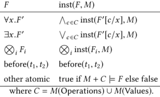
F inst(F, M) ∀x .F′ Ó c ∈Cinst(F′[c/x], M) ∃x .F′ Ô c ∈Cinst(F′[c/x], M) Ë iFi Ëiinst(Fi, M) before(t1, t2) before(t1, t2)

other atomic true if M+ C |= F else false whereC = M(Operations) ∪ M(Values).

Fig. 3. The instantiation of a formula F with model M defined recursively, where C is the finite set of operations and values occurring in M,Ë is an arbitrary logical connective, e.g., ¬, ∧, ∨, and M+ C denotes the model obtained from M by adding identity interpretations for the constants C.

More technically, the instantiation of a history formulaF with a history model M is the formula inst(F ∧ Θ, M) ∧ ord(M), where Θ are the axioms of total order on before:

∀x, y, z. before(x, y) ∧ before(y, z) ⇒ before(x, z), ∀x, y. x = y ∨ before(x, y) ∨ before(y, x), and ∀x, y. ¬before(x, y) ∨ ¬before(y, x),

inst(F ∧ Θ, M) is defined by Figure3, and ord(M) is the conjunction of happens-before constraints

fromM:

{before(o1, o2) :M(before)(o1, o2)}.

Essentially, inst(F, M) replaces the quantified variables of F with the operations and values of M, and replaces atomic formulas unrelated to order with Boolean constants.

An operation-order formula is said to have a total-order axiomatization if it either: • contains the above axiomsΘ of total order on before, or

• is ground, quantifier-free, and contains the matrixΘ′of the above axioms instantiated via Θ′

[o1/x][o2/y][o3/z] for every triple of operation-sort constants o1, o2, o3occurring within3.

Intuitively, when formulas contain total-order axiomatization we may treat the before predicate as uninterpreted since any satisfying model must map before to a total order.

The following lemmas demonstrate that instantiation is an effective reduction from the safety of a history model to the satisfiability of an operation-order formula.

Lemma 5.3. The instantiation of a history formulaF is a ground and quantifier-free operation-order formula with total-order axiomatization computable in polynomial time for any fixed quantifier rank formulaF .

Proof. The instantiation being a ground and quantifier-free operation-order formula with total-order axiomatization is a direct consequence of the definition. For a given history modelM, it is computable in time O(nmax(k,3)_{· |F |) where n is the number of operations and values in M, |F | is}

the size of the formulaF , and k is its quantifier rank. □ Lemma 5.4. The instantiation of a history formulaF can be transformed to conjunctive normal form in polynomial-time for any fixed quantifier rank formulaF .

3_{These instantiations will contain only before atoms. The equality in the second axiom of Θ will be replaced by a boolean}

Proof. The instantiation of a history formulaF of quantifier rank k (assumed to be in CNF) contains at mostk + 2 nestings of boolean operators which can be distributed to produce a CNF formula in time O(nmax(k,3)_{· |F |). □}

Lemma 5.5. The instantiation of a history formulaF with history model M is satisfiable iff M is safe forF .

Proof. A modelM is safe for F iff there exists a total extension Ms ofM such that Ms |= F. SinceMs differs withM just in the interpretation of before, and the interpretation of the latter inMs is consistent with its interpretation inM, we have that Ms |= inst(F ∧ Θ, M) ∧ ord(M).

Also, by definition, any model of inst(F ∧ Θ, M) ∧ ord(M) is a total extension of M (the total order axiomatization included in inst(F ∧ Θ, M) ensures that before is interpreted as a total order). Therefore,M is safe for F iff inst(F ∧ Θ, M) ∧ ord(M) is satisfiable. □ To further reduce the satisfiability of operation-order formulas to propositional Horn satisfiability, we suppose that formulas are in conjunctive normal form. Then let ∼ be the minimal equivalence relation on literals includingp(t1, t2) ∼ ¬p(t2, t1) for any predicatep and terms t1, t2. Intuitively,

the ∼ relation relates literals that are equivalent under the assumption thatp is an antisymmetric order with totality since ¬p(t2, t1) would implyp(t1, t2) and vice versa for termst1, t2. Extending ∼

to clauses, we relate two equal-length clausesÔ {l0, . . . , ln} ∼Ô {l0′, . . . , l ′

n} whenli ∼l_i′for each 0 ≤i ≤ n. The Hornification of a quantifier-free operation-order formula F = Óci in conjunctive normal form is the formula

Û

{c : ∃i. c ∼ c_i andc is Horn}, of all Horn clausesc related to some clause ci ofF .

Example 5.6. The Hornification of the non-Horn clause

before(o1, o2) ∨ before(o2, o4) ∨ ¬before(o1, o4),

is the following set of clauses,

before(o1, o2) ∨ ¬before(o4, o2) ∨ ¬before(o1, o4),

¬before(o2, o1) ∨ before(o2, o4) ∨ ¬before(o1, o4),

¬before(o2, o1) ∨ ¬before(o4, o2) ∨ ¬before(o1, o4),

¬before(o2, o1) ∨ ¬before(o4, o2) ∨ before(o4, o1),

which are in Horn form. All clauses are equivalent in theories where before is a total order. The following lemmas demonstrate that Hornification is an effective reduction from satisfiability to Horn satisfiability of operation-order formulas.

Lemma 5.7. The Hornification of a ground and quantifier-free operation-order formula in conjunctive normal form with total-order axiomatization is a ground, quantifier-free, and Horn operation-order formula.

Proof. Follows by definition of Hornification. □ Lemma 5.8. The Hornification of an operation-order formula is polynomial-time computable. Proof. Without loss of generality, we assume a fixed maximum clause lengthk > 2; any cnf formula can be rewritten to one with maximum clause lengthk in polynomial-time. In more details, every clausec of length m can be split into a conjunction of O(m/k) clauses of length k that use O(m/k) additional variables to ensure that one of the literals in c is true iff there exists an assignment

for the additional variables such that all thek-length clauses are true. This transformation leads to an equivalent formula modulo the interpretation of the additional variables. Given a formula with n clauses of maximum clause length k, any given clause has O(2k_{) possible clauses related by ∼,}

and thus the number of clauses in the Hornification is limited by O(n · 2k_{), which reduces to O(n)}

for fixedk. □

The following result shows that the HornificationF′of a quantifier-free operation-order formula F with total-order axiomatization is equisatisfiable to F . We remark that these formulas are generally not equivalent, sinceF′_{may have models in which before is interpreted to a partial order, while F}

only has total models, since it has a total-order axiomatization.

Lemma 5.9. The Hornification of a ground and quantifier-free operation-order formulaF in con-junctive normal form with total-order axiomatization is satisfiable iffF is satisfiable.

Proof. SinceF is ground and quantifier-free, its satisfiability can be decided using a derivation based on the resolution rule of propositional logic (each atom is viewed as a boolean variable). We prove that any such derivation that uses as axioms clauses inF and derives a clause c can be rewritten to a derivation that uses as axioms clauses in the Hornification ofF and derives a clausec′withc ∼ c′. Instantiating this fact forc being the empty clause we get that F is satisfiable when its Hornification is satisfiable. The other direction is trivial since the clauses added in the Hornification ofF can be always derived by the resolution rule from clauses in F .

W.l.o.g. we assume that all the clauses inF except those which express totality, i.e., the clauses of the form before(o1, o2) ∨ before(o2, o1), are Horn. Otherwise, every other non-Horn clausec can

be replaced with some Horn clausec′such thatc′∼c. The obtained formula is equivalent to the original one.

LetF denote the Hornification of F , and F ⊢ c denote a derivation based on the resolution rule which uses as axioms clauses inF and derives the clause c. We prove that for every such formula F and every derivationF ⊢ c,

there existsF ⊢ c′for all Horn clausesc′_withc′_{∼c. (1)}

We proceed by induction on the numberN of non-Horn resolvents in F ⊢ c. We write F ⊢N c for

a derivation withN non-Horn resolvents.

Base case: A non-empty derivationF ⊢0c may contain non-Horn clauses only as axioms, and the

conclusionc is necessarily a Horn clause (we omit the case of empty derivations which is trivial). Consider an application of the resolution rule in this derivation with at least one non-Horn clause as premise (c1andc2are clauses anda is an atom):

c1∨a c2∨ ¬a

c1∨c2

We calla the pivot of the resolution rule application.

By hypothesis,c1∨c2is Horn and must contain exactly one positive literalb (if it contains no

positive literal, then both premises are Horn). This positive literal must belong toc1(otherwise,

both premises are Horn:c1∨a contains no positive literal other than a, and c2∨ ¬a contains only

b as a positive literal). Therefore, c1∨a is a clause expressing totality of the form b ∨ a with b ∼ ¬a

and the derivation rule becomes:

b ∨ a c2∨ ¬a

Sincec2cannot contain other positive literal thanb and b ∼ ¬a, the conclusion b ∨ c2of this rule is

included inF . Therefore, replacing all such resolution rule applications with axioms from F , the derivationF ⊢0c can be transformed to a derivation F ⊢ c′for somec′∼c.

To conclude, we prove that a derivationF ⊢ c′_{for some Horn clausec}′_{∼c can be rewritten}

to a derivationF ⊢ c′′_{for every Horn clausec}′′_∼c′_{. Whenc}′′_{is obtained fromc}′_{by replacing}

a positive literala with ¬b such that a ∼ ¬b, the same transformation can be applied to all the resolvents in the derivationF ⊢ c′_{and obtain a new derivationF ⊢ c}′′_{(a Horn clause remains Horn}

when a positive literal is replaced by a negative one). Next, w.l.o.g., assume thatc′′_{is obtained from}

c′

by replacing a positive literala with ¬b and a negative literal ¬a′withb′such thata ∼ ¬b and ¬a′_∼b′

. We proceed by induction on the number of applications of the resolution rule inF ⊢ c′. W.l.o.g., assume that the last application of the resolution rule is of the form:

a ∨ c1∨ ¬d ¬a′∨c2∨d

a ∨ c1∨ ¬a′∨c2

wherec1andc2are clauses that contain only negative literals. This rule can be rewritten as follows

¬b ∨ c1∨d′ b′∨c2∨ ¬d′

¬b ∨ c1∨b′∨c2

where ¬d′_{∼d. Applying also the induction hypothesis, we get that there exists a derivation F ⊢ c}′′

. Induction step: Assume that (1) holds for all derivations withN non-Horn resolvents, and let F ⊢_{N +1}c be a derivation. Let

c1∨a c2∨ ¬a

c1∨c2

be an application of the resolution rule inF ⊢N +1c such that all the resolvents in the derivation of

the premisesc1∨a and c2∨ ¬a are Horn and c1∨c2is not Horn. The latter derivation may still

contain other non-Horn clauses than the conclusion, but they are necessarily axioms.

One of the premises above must be a resolvent (since the only non-Horn axioms are those expressing totality, and two such axioms can’t be the premises of the same derivation rule). Also, remark thatc1∨a and c2∨ ¬a can’t be both Horn clauses (otherwise, c1∨c2would be Horn). Also,

the non-Horn clause between the two is necessarily an axiom by the choice of the resolution rule application. Therefore,c1∨a is an axiom expressing totality of the form b ∨ a with b ∼ ¬a and the

derivation rule becomes:

b ∨ a c2∨ ¬a

b ∨ c2

Ifb is not the pivot of a further resolution rule application, then this rule is vacuous and it can be eliminated. More precisely, all the further applications of the resolution rule are enabled ifc2∨ ¬a

is considered instead ofb ∨ c2. Eliminating this application will lead to a derivation with at mostN

non-Horn resolvents for which the induction hypothesis holds.

Assume now thatb is the pivot of a further resolution rule application. The derivation F ⊢_{N +1}c can be then outlined as (Axi withi ∈ [1, 4] are sets of axioms):

b ∨ a Ax1 ·· ·· · c2∨ ¬a c2∨b ·· ·· · Ax2 ·· ·· · c3∨b Ax3 ·· ·· · c4∨ ¬b c3∨c4 Ax4 ·· ·· · c

Applying the induction hypothesis for the derivationsAx1⊢0c2∨ ¬a and Ax3⊢N′c₄∨ ¬b with

N′_{≤N , we get that there exist derivations Ax}

1⊢c₂′∨ ¬a and Ax3⊢c₄′∨a for some Horn clauses

c′

2∨ ¬a ∼ c2∨ ¬a and c4′∨a ∼ c4∨ ¬b. The derivation F ⊢N +1c can be transformed as follows:

Ax1 ·· ·· · c′ 2∨ ¬a Ax3 ·· ·· · c′ 4∨a c′ 2∨c ′ 4 ·· ·· · Ax2 ·· ·· · c′ 3∨c ′ 4 Ax4 ·· ·· · c′

This transformed derivation is correct because of the following:

• {c2∨b} ∪ Ax2 ⊢N′c₃∨b with N′≤N implies {c₂} ∪Ax₂ ⊢_N′c₃. Then, by the induction

hypothesis, there exists a derivation {c2} ∪Ax2⊢c3′for somec ′ 3∼c3.

• since increasing the set of literals in the premises doesn’t disable any resolution rule applica-tion, we get that there exists a derivation {c2∨c4′} ∪Ax2⊢c3′∨c

′ 4.

• for simplicity, assume thatc′ 2∨c

′

4is the only axiom in the latter derivation which belongs

to {c2∨c₄′}. We get thatAx1∪Ax2∪Ax3⊢c₃′∨c₄′. If the simplifying assumption doesn’t

hold, then the derivation ofc′ 3∨c

′

4would contain derivations of other Horn formulas in

{c2∨c₄′}. These derivations can be obtained trough a trivial rewriting from the derivation of

Ax1∪Ax3⊢c2′∨c ′ 4.

• finally, since {c3 ∨c4} ∪Ax4 ⊢N′ c with N′ ≤ N we get that there exists a derivation

{c3∨c4} ∪Ax4⊢c′for somec′∼c. Again, we can assume for simplicity that c₃′∨c₄′is the

only axiom in these derivations which belongs to {c3∨c4}. Otherwise, we can proceed as in

the previous case.

This transformed derivation has axioms fromF and derives a Horn clause c′_{∼c. Such a derivation}

can be rewritten to a derivationF ⊢ c′′_{for every Horn clausec}′′_∼c′_{. This concludes our proof. □}

The proof of Lemma5.9relies on a stronger property of the Hornification: any Horn clausec derived in a resolution proof from the original formulaF can be also derived from the Hornification

ofF . (The reverse holds trivially since any clause added to the Hornification can be derived from the clauses ofF .) When c is the empty clause, this property amounts to equisatisfiability. Looking at the first steps in a derivation ofc from F , a resolution rule application that uses as a premise an instance of the totality axiom corresponds to replacing an atom ¬p(t1, t2) withp(t2, t1). This transformation

is in principle anticipated with the new clauses added in the Hornification ofF . However, the restriction to Horn clauses may force other atoms to be replaced with equivalent counterparts. Therefore, replacing that resolution rule application with a clause from the Hornification may affect other parts of the derivation as well. Nevertheless, these parts of the derivation can be rewritten using again clauses from the Hornification.

Combining instantiation, Hornification, and propositional Horn satisfiability yields an efficient procedure for oos linearizability. Its asymptotic complexity is dominated by quantifier instantiation which is O(nk_{), wherek is the rank of the input operation-order signature.}

Theorem 5.10. oos linearizability is solvable in polynomial time for fixed-rank operation-order signatures.

Proof. Given an operation-order specification ⟨Σ, I, F0, R⟩ and a history h, from the definitions

of history interpretation and operation-order specification we obtain a history modelI(h) in polynomial time which is safe withF0iffh is oos linearizable. By Lemmas5.3–5.9, we know that

I(h) is safe with F0 iff the polynomial-time instantiationF1 ofF0withI(h) is satisfiable, which

in turn is satisfiable iff the polynomial-time HornificationF2ofF1is satisfiable. Constructing a

propositional Horn formulaF3fromF2by replacing each atom before(o1, o2) with a propositional

variablexo1,o2, it follows thatF3 is equisatisfiable toF2, and by Lemma5.2, its satisfiability is

polynomial-time computable. □

The remaining sections demonstrate that oos linearizability amounts to a sound decision proce-dure for linearizability of collection types.

6 COMPLETE COLLECTION-VIOLATION PATTERNS

In this section we demonstrate the fundamental combinatorial properties enjoyed by collection types enabling our reduction to oos linearizability. Essentially, we show that any violation to a collection in an unambiguous sequence (see Section3) can always be reduced to one of a finite number of violation patterns. More technically, we characterize violations via an embedding relation between unambiguous sequences, and demonstrate that this relation always yields a bounded set of minimal sequences of which every violation embeds at least one. Later, in Section7, we demonstrate that this minimal set of violation patterns defines the history formula of an operation-order specification against which the linearizability of a given sequence is judged.

Our embedding relation is built from three smaller relations →s, →r, and →v, relating

operation-label sequencess1ands2whens2is obtained froms1by,

• applying a substitution (→s),

• removing a read-only operation (→r), or

• removing all operations which touch a given value (→v).

Our embedding relation ⊒ is the smallest reflexive and transitive binary relation containing →s,

→_r, and →v. The embedding relatess1⊒σ(s2) for any substitutionσ, where s2is obtained from

s1 by removing all operations touching any given set of values, and any number of read-only

operations. Violations to a collection are characterized by this embedding relation in the sense that any unambiguous sequences1which embeds a violations2(i.e.,s1 ⊒σ(s2)) is also a violation (see

Lemma6.6). For instance, adding read-only operations to a violations2results in a sequences1

Example 6.1. The embedding relation ⊒ relates the following unambiguous sequences of decreas-ing length

push(1) · push(2) · push(3) · pop ⇒ 3 · peek ⇒ 2 · pop ⇒ 1 →v push(1) · push(2) · peek ⇒ 2 · pop ⇒ 1

→r push(1) · push(2) · pop ⇒ 1

→s push(3) · push(4) · pop ⇒ 3,

neither of which are admitted by the stack type.

We show that the embedding relation ⊑ has a finite set of minimal elements when restricted to the set of sequences that touch a bounded set of values and where the number of mutators (non-readonly operations) that touch a given value is also bounded. This property is captured formally with wqos: a well-quasi-ordering (wqo)Q on a set X is a reflexive, transitive binary relation onX for which in every infinite sequence x0x1. . . of elements from X , there exists indices i < j

such thatQ(xi, xj).

For a local type, a valuev is k-valent in a sequence s when |touches∗(s,v) ∩ ¬readonly∗(s)| ≤ k, and a sequences is k-valent when all values are k-valent in s. A sequence s is k-valued if at most k unique input or output parameters occur within, i.e., |Ò

ivals(si)| ≤k. We write Vkto denote the set of sequences which are bothk-valent and k-valued.

Example 6.2. All the sequences in Example6.1are 2-valent since the only mutators touching a given value are push and pop. Moreover, they all belong toV3since they are 3-valued.

Lemma 6.3. ⊑ is a wqo onVkfor all local types andk ∈ N.

Proof. Let (si)_{i ∈N} be an infinite sequence4 _{of sequences fromV}

k. SinceVk is closed under

value substitution, there exists a set of valuesV with |V | ≤ k and conflict-free substitutions σi

with rangeV such that s_i′ = σi(si) ∈ V_k. Letµ be a map from sequences s to multisets µ(s) = {s(j) : j ∈ (¬readonly)∗_{(s)} of non-readonly labels. Since T is local, the labels of the s}′

i sequences

come from a finite set. Moreover, thes_i′sequences arek-valent which implies that the range of possible multisetsµ(s_i′) is bounded. It follows that there exists an infinite subsequence (s_i′)i ∈I for I ⊆ N of operation-label sequences with the same mutator multiset, i.e., µ(s′

i1) = µ(s ′

i2) for all

i1, i2 ∈ I. By Higman’s Lemma, the subsequence order is a wqo on sequences from a bounded

interface, which guarantees the existence ofi1, i2∈I such that i1< i2andsi′1is a subsequence of

s′

i2. Since the mutators ofs ′ i1ands

′

i2are identical, it follows thats ′ i1= s ′ i2ors ′ i1is obtained froms ′ i2

by removing only read-only operations. By the definition of (s′

i)i ∈N, we get thatσi1◦σ −1 i2 (s ′ i1) is a subsequence ofs_i′ 2and thatσi1◦σ −1 i2 (s ′ i1) is obtained froms ′

i2by removing only read-only operations.

Thussi1⊑si2. □

Given an abstract data typeT , we write Pk to denote a minimal set of ⊑-minimal sequences

representing ¯T ∩ Vk, i.e., such thats ∈ (Vk\T ) iff there exists s′∈Pk withs′⊑s. Intuitively, any

violation to the data typeT that belongs to Vkwill embed one of the sequences inPk, referred to

also as violation patterns.

4_{To avoid confusion here we writes}

ito denote theith operation-label sequence in a sequence s0s1. . . of operation-label

Example 6.4. IfT is the stack type with push and pop operations, then P2consists of

pop ⇒ 1

pop ⇒ 1 · push(1)

push(1) · pop ⇒ 1 · pop ⇒ 1 push(1) · push(2) · pop ⇒ 1

push(1) · push(2) · pop ⇒ 1 · pop ⇒ 2

By Lemma6.3the setPkis finite. It can be effectively computed by tracking minimal elements within sequences inVkover a fixed set ofk values and with at most one readonly operation5whose number is bounded byk2_{+ 1 (there are at most k mutators that can touch one of the k values).}

Corollary 6.5. Pkcontains at mostk2+ 1 elements and it is computable.

For the remainder we fix a minimalPk. We show that any sequence that embeds one of the

patterns inPk, for anyk, is a violation to a local and parametric abstract data type. To this, we

introduce a weakening of locality, called partitionability, that is enough to conclude this fact (together with parametricity).

An abstract data typeT is partitionable when s′∈T whenever s ∈ T for some s′⊑s. Note that any partitionable type is also parametric sinceσ(s) ⊑ s for all s.

Lemma 6.6. Local parametric types are partitionable.

Proof. LetT be a local parametric type, s a sequence in T , and s′ ⊑s for some sequence s′. W.l.o.g., we assume thats′→ss, s′→rs or s′→vs. The case s′→ss follows directly from the fact

thatT is parametric. Ifs′ _→

rs, then there exist sequences s1ands2, and operation label ℓ, such thats = s1·ℓ · s2,

s′_{= s}

1·s2, and readonly(s1·ℓ) holds. By the definition of the readonly predicate, s1·ℓ and s1are

equivalent and thus,s1·ℓ · s2 ∈T iff s1·s2 ∈T . Therefore, s′∈T .

Whens′_→

vs, the fact that s′∈T can be proved by induction on the length of s. By definition,

s′_{is obtained froms by removing the labels on positions J = touches}∗_{(s,v) for some value v.}

Essentially, there are two cases two consider.

case 1: Ifs ends with a label that touches v, i.e., |s| − 1 ∈ J, then s without that label is still admitted byT (by prefix closure) and the induction hypothesis applies.

case 2: Otherwise, we haves = s1·ℓ for some sequence s1and label ℓ, such that ¬uses(s1·ℓ,v).

Therefore, drop(s1,v)·ℓ ∈ T . Since T is local, we have that v < vals(ℓ) which implies drop(s1,v)·ℓ =

drop(s,v), and that J = {i : v ∈ vals(si)} which implies drop(s,v) = s′. Hence,s′∈T . □ LetEkbe the set

Ek = {s : ∃s′∈Pk. s′⊑s}

of sequences which embed one of the patterns inPk. When the abstract data typeT is parametric

and partitionable,Ekcontains only sequences which are not admitted byT . Lemma 6.7. IfT is parametric and partitionable and s ∈ Ekthens < T .

Proof. Given a sequences ∈ Ek there exists a ⊑-minimal sequences′∈Pksuch thats′⊑s, and by definition of ⊑ it follows thats′= σ(s′′) for some subsequences′′ofs and substitution σ. By definition ofPk we knowσ(s′′) < T , and then s′< T since T is parametric by hypothesis. Finally s < T since T is partitionable and s′′_{⊑s by definition of ⊑.}

□

We strengthen the result in Lemma6.7by showing that there exists somek such that Ekcontains

exactly all the unambiguous sequences which arek-valent and violations to a given collection. Proving also that all the unambiguous sequences which are notk-valent for some k ≥ 2 are violations to a given collection leads to a characterization of unambiguous violations that is describable using a history formula.

A set of sequencesX is Vk-reducible ifs ∈ X whenever s is k-valent and s′∈X for all s′∈Vk

such thats′⊑s.

Lemma 6.8. The set of unambiguous sequences admitted by a collection are 2-valent.

Proof. Lets be a unambiguous sequence admitted by a collection T . Because T is value-invariant, for any label ℓ ins such that touches(ℓ,v) ∧ ¬readonly(ℓ) holds for some value v, we have that adds(ℓ,v) ∨ removes(ℓ,v) holds. Then, since s is unambiguous, there exists at most one label ℓ such that adds(ℓ,v) holds. This implies that there exists at most one label satisfying removes(ℓ,v), and

thuss is 2-valent. □

Lemma 6.9. The set of unambiguous sequences admitted by a collection isVk-reducible for some k ≥ 2.

Proof. Lets be a unambiguous sequence, i.e., adds(ℓ,v) holds for at most one label ℓ in s, for each valuev, and T a collection. Lemma6.8shows thats ∈ T implies that s is 2-valent. Then, since T is reducible, there exists some bound k such that s ∈ T whenever keep(s,V ) ∈ T for every subset V ⊆ vals(s) of size |V | ≤ k. W.l.o.g., assume that k ≥ 2. Indeed, by definition, if T is reducible with some boundk then it is reducible with any greater bound k′ ≥k. We have that keep(s,V ) ⊑ s becauseT is local, i.e., every operation touches exactly the values appearing in its label. Moreover, ifs is k-valent, then all the subsequences keep(s,V ) are k-valent which concludes the proof. □ A local abstract data typeT has bounded violations in unambiguous sequences when there exists some boundk ≥ 2 such that for every unambiguous sequence s, we have that s < T iff s is not k-valent or s ∈ Ek.

Theorem 6.10. Every collectionT has bounded violations in unambiguous sequences.

Proof. We have to show that for every unambiguous sequences, s < T iff s is not k-valent or s ∈ Ek. The “if” direction holds from Lemmas6.6,6.7, and6.8. For the “only-if” direction, Lemma6.9

implies that the set of unambiguous sequences isVk-reducible, for somek. Therefore, for any

unambiguous sequences < T , either s is not k-valent, or there exists a sequence s′_∈V

kwiths′⊑s

such thats′

< T . Since s′∈ ( ¯T ∩ Vk) there exists a ⊑-minimal sequences′′∈Pksuch thats′′⊑s′,

and thuss′′_{⊑s because ⊑ is transitive. Then s ∈ E}

kby definition ofEk. □

The next section uses the result in Theorem6.10to define a history formula that describes precisely the unambiguous sequences admitted by a collection, which is the essential ingredient of a sound operation-order specification.

7 SOUND OPERATION-ORDER SPECIFICATIONS

In this section we leverage the combinatorial properties of Section6to demonstrate that collection types have sound operation-order specifications. We construct these specifications automatically given a set of violation patterns and a local interpretation for the operation predicates of a given collection type — both which could be inferred usingEmmi and Enea[2016]’s algorithm for extracting patterns from execution samples. The specifications use a restriction to unambiguous histories, and extend the basic history signature with the operation predicates of collection types. The extended signature is interpreted using the local interpretation for a given type, and history