Contributions à la simulation stochastique parallèle : architectures logicielles pour la distribution de flux pseudo-aléatoires dans les simulations Monte Carlo sur CPU/GPU

Texte intégral

(1)Contributions to parallel stochastic simulation : application of good software engineering practices to the distribution of pseudorandom streams in hybrid Monte Carlo simulations Jonathan Passerat-Palmbach. To cite this version: Jonathan Passerat-Palmbach. Contributions to parallel stochastic simulation : application of good software engineering practices to the distribution of pseudorandom streams in hybrid Monte Carlo simulations. Software Engineering [cs.SE]. Université Blaise Pascal - Clermont-Ferrand II, 2013. English. �NNT : 2013CLF22383�. �tel-01980715�. HAL Id: tel-01980715 https://tel.archives-ouvertes.fr/tel-01980715 Submitted on 14 Jan 2019. HAL is a multi-disciplinary open access archive for the deposit and dissemination of scientific research documents, whether they are published or not. The documents may come from teaching and research institutions in France or abroad, or from public or private research centers.. L’archive ouverte pluridisciplinaire HAL, est destinée au dépôt et à la diffusion de documents scientifiques de niveau recherche, publiés ou non, émanant des établissements d’enseignement et de recherche français ou étrangers, des laboratoires publics ou privés..

(2) Contributions to parallel stochastic simulation: Application of good software engineering practices to the distribution of pseudorandom streams in hybrid Monte-Carlo simulations by. Jonathan Passerat-Palmbach A Thesis submitted to the Graduate School of Engineering Sciences of the Blaise Pascal University - Clermont II in fulfilment to the requirements for the degree of. Docteur of Philosophy in Computer Science Supervised by David R. C. Hill at the LIMOS laboratory - UMR CNRS 6158 publicly defended on October, 11th 2013 Committee: Reviewers: Supervisor: Chairman: Examiners:. Pr. Pr. Pr. Pr. Pr. Pr. Dr. Dr.. Michael Mascagni Stéphane Vialle David R. C. Hill Alain Quillot Pierre L’Ecuyer Makoto Matsumoto Bruno Bachelet Claude Mazel. -. Florida State University, USA Supélec, Campus de Metz, France Blaise Pascal University, France Blaise Pascal University, France Montreal University, Canada Hiroshima University, Japan Blaise Pascal University, France Blaise Pascal University, France.

(3)

(4) Abstract. The race to computing power increases every day in the simulation community. A few years ago, scientists have started to harness the computing power of Graphics Processing Units (GPUs) to parallelize their simulations. As with any parallel architecture, not only the simulation model implementation has to be ported to the new parallel platform, but all the tools must be reimplemented as well. In the particular case of stochastic simulations, one of the major element of the implementation is the pseudorandom numbers source. Employing pseudorandom numbers in parallel applications is not a straightforward task, and it has to be done with caution in order not to introduce biases in the results of the simulation. This problematic has been studied since parallel architectures are available and is called pseudorandom stream distribution. While the literature is full of solutions to handle pseudorandom stream distribution on CPUbased parallel platforms, the young GPU programming community cannot display the same experience yet. In this thesis, we study how to correctly distribute pseudorandom streams on GPU. From the existing solutions, we identified a need for good software engineering solutions, coupled to sound theoretical choices in the implementation. We propose a set of guidelines to follow when a PRNG has to be ported to GPU, and put these advice into practice in a software library called ShoveRand. This library is used in a stochastic Polymer Folding model that we have implemented in C++/CUDA. Pseudorandom streams distribution on manycore architectures is also one of our concerns. It resulted in a contribution named TaskLocalRandom, which targets parallel Java applications using pseudorandom numbers and task frameworks. Eventually, we share a reflection on the methods to choose the right parallel platform for a given application. In this way, we propose to automatically build prototypes of the parallel application running on a wide set of architectures. This approach relies on existing software engineering tools from the Java and Scala community, most of them generating OpenCL source code from a high-level abstraction layer. Keywords: Pseudorandom Number Generation (PRNG); High Performance Computing (HPC); Software Engineering; Stochastic Simulation; Graphics Processing Units (GPUs); GPU Programming; Automatic Parallelization.

(5)

(6) Acknowledgements / Remerciements. “Anyone who ever gave you confidence, you owe them a lot. — Truman Capote, Breakfast at Tiffany’s. First of all, I’d like to thank all the members of my committee for having accepted to evaluate my work, read this thesis and attend my defence. Merci à David, mon directeur de thèse, qui a été si présent durant ces 3 années (et même avant). Il a su trouver la bonne formule pour guider mon travail et me permettre d’atteindre mes objectifs, tant professionnels que personnels. Son soutien permanent en fait un proche que j’ai besoin de quitter pour grandir, mais envers qui ma reconnaissance est sans limite. Dans le même esprit, je tiens à évoquer Laurent, mon entraîneur qui me suit depuis tant d’années, qui m’a emmené là où je suis sportivement et humainement. Je lui associe mes succès présents et futurs, et où que je sois, il restera une présence inamovible pour mon équilibre. Après avoir évoqué mes 2 “pères spirituels”, je ne peux qu’évoquer mon père, qui croit tellement en moi depuis toujours, qui m’a donné goût au voyage et à la découverte, et dont le regard sur ce que je fais est si important pour moi. À ton tour, mère, de recevoir mes pensées. Toi qui m’a poussé vers le sport étant jeune, et qui aujourd’hui est un soutien sans faille, peu importe mes résultats ou mes performances, tout ce que tu fais pour moi n’a pas de prix. Je me tourne à présent vers les personnes qui ont guidé mes choix, m’ont passionné et donné envie d’aller dans cette direction plutôt qu’une autre. Je pense à Guénal, François, Sylvie, Michel, Olivier, Édith, Murielle, Philippe et Alain. Mais aussi les “grands frères” : Paul, Paul (encore), Romain, Guillaume et Julien..

(7) iv. Acknowledgements / Remerciements. Cette thèse ne serait pas là sans mes amis présents au quotidien, au travail, à l’entraînement et pour les extras, merci à vous tous de me supporter moi et mon emploi du temps. Un hommage donc à Guillaume, futur associé potentiel, doctorant, machine à écrire et pokéfan; Florian, compagnon de voyage, de billard et de débat philosophiques, dont l’hyperactivité m’épuiserait presque parfois; Jean-Baptiste, mon binôme de toujours, dans les mauvais mais surtout les très bons moments; Lorena, qui m’a donné sa confiance, et fait preuve d’une patience infinie; Nicolas, que j’aime même s’il contribue à tuer des gens, expert en discussion par boîte vocales interposées; Thomas, que j’ai découvert sur le tard, mais qui me fait partager son expérience et surtout ses bonnes histoires; Nicolas (l’autre), soirée foot ou soirée tout court, même délires, mêmes histoires, parfait! Sébastien, ancien co-bureau, actuel co-détenteur du record de présence au labo une veille de Noël; Nathalie, dont je loue la capacité à nous supporter jour après jour; Luc, source intarissable de connaissances informatiques et cascadeur amateur; Jonathan, co-auteur du “bijou”, qui m’a transmis un échantillon de sa rigueur légendaire (petit jeu : il y a un double espace dans ce document); Pierre, le jeune, co-bureau plein d’avenir et de talent, a révélé en moi une vocation d’agent immobilier; Romain, ma conscience, même parti je me demande toujours ce que tu penserais; Clément, mon petit frère, polyglotte notoire dans certains champs lexicaux; Christine, que je ne vois que trop peu souvent; Hélène, cuisinière hors-pair, toujours proche de moi malgré la distance; Benoît, premier contact humain sur le campus, premier retard en cours, toujours là; Faouzi, ami des biologistes, déménageur amateur à mes côtés; Wajdi, my bro! ou Dracula, compagnon de nuit au labo, prétend être tunisien, même si tout le monde sait qu’il est norvégien; Yannick, mon premier stagiaire, développeur de talent, globe-trotter, ogre à sushi; Isaure, ma jumelle, pas besoin de parler pour savoir ce qu’il en est; Lionel, éclaireur de tous les chemins que j’emprunte, apprenti-jardinier; Cédrick, l’homme qui défie la chance, me suivrait jusqu’au bout du monde pour se casser un membre; David, mon exemple de motivation, travaille sans relâche mais trouve toujours du temps pour m’emmener dans des soirées improbables; Romina, ces 10 années de correspondance me donnent l’impression que tu es si proche ma Suissesse; Mathilde, fauve insaisissable parfois, énervante souvent, passionnante tout le temps; Audrey, y’a-t-il quelque chose au-delà de meilleure amie pour représenter ton importance ? Sarah, qui a visiblement su trouver les mots et l’accent pour se faire une place, étonne-moi aussi longtemps que tu le souhaites. Je tiens à présent à remercier mes collègues de travail à l’ISIMA, au LIMOS ou dans d’autres équipes, avec une pensée particulière pour Claude, Bruno et Ivan qui ont joué un rôle majeur dans le travail que je présente. Merci aussi à Loïc, Antoine, Firmin, Violaine, Romuald, Christophe, Corinne, Susan, Béatrice, Françoise et Séverine pour.

(8) Acknowledgements / Remerciements. v. leur soutien et leur bonne humeur qui ont rendu les journées de travail (et les nuits pour certains) très agréables. Dédicace au passage à tous ceux qui n’ont pas cru en moi, preuve s’il en faut qu’on ne gagne pas à tous les coups. Pour Elles, je laisse parler Baudelaire. . . Vous que dans votre enfer mon âme a poursuivies, Pauvres sœurs, je vous aime autant que je vous plains, Pour vos mornes douleurs, vos soifs inassouvies, Et les urnes d’amour dont vos cœurs sont pleins. Un mot enfin pour tous ceux que, pressé par le temps, j’ai oublié de citer mais qui ont compté tout au long de mon parcours. Plus généralement, merci à tous pour votre tolérance quant à mes retards chroniques, mais les hommes libres de Jarry ne m’ont que trop inspiré : “La liberté, c’est de ne jamais arriver à l’heure” !.

(9)

(10) Contents Abstract. i. Acknowledgements / Remerciements. iii. Introduction. 1. 1 Parallel Pseudorandom Numbers at the Era of GPUs. 5. 1.1. Parallel Stochastic Simulation and Random Numbers . . . . . . . . . .. 6. 1.2. About Random Numbers . . . . . . . . . . . . . . . . . . . . . . . . . .. 7. 1.2.1. Pseudorandom Numbers . . . . . . . . . . . . . . . . . . . . . .. 7. 1.2.2. Why do we settle for Pseudorandom Numbers when True Random Numbers are available? . . . . . . . . . . . . . . . . . . . .. 7. 1.3. Pseudorandom Number Generation in parallel . . . . . . . . . . . . . .. 10. 1.4. Pseudorandom streams on GPU . . . . . . . . . . . . . . . . . . . . . .. 11. 1.5. Details about GPUs: programming and architecture . . . . . . . . . . .. 13. 1.5.1. Architecture . . . . . . . . . . . . . . . . . . . . . . . . . . . . .. 13. 1.5.2. Programming model of NVIDIA GPUs . . . . . . . . . . . . . .. 16. 1.5.3. Programming languages . . . . . . . . . . . . . . . . . . . . . .. 19. On the need for software engineering tools . . . . . . . . . . . . . . . .. 22. 1.6.1. Software Engineering . . . . . . . . . . . . . . . . . . . . . . . .. 22. 1.6.2. Object-Oriented Modelling . . . . . . . . . . . . . . . . . . . . .. 22. 1.6.3. Template MetaProgramming . . . . . . . . . . . . . . . . . . . .. 24. 1.6. 2 PRNG in Parallel Environments: the Case of GPUs 2.1. Introduction . . . . . . . . . . . . . . . . . . . . . . . . . . . . . . . . .. 25 26.

(11) viii. Contents. 2.2. Statistical and Empirical Testing Software for Random Streams . . . .. 27. 2.3. Design of Parallel and Distributed Random Streams . . . . . . . . . . .. 29. 2.3.1. Partitioning a unique original stream . . . . . . . . . . . . . . .. 29. 2.3.2. Partitioning multiple streams: Parameterization . . . . . . . . .. 33. 2.3.3. Other techniques . . . . . . . . . . . . . . . . . . . . . . . . . .. 34. 2.3.4. A tool for partitioning: jump-ahead algorithms . . . . . . . . .. 35. 2.3.5. Joint use of the partitioning of a single stream and parameterization 35. 2.4. 2.5. 2.6. Pseudorandom Numbers on GPUs . . . . . . . . . . . . . . . . . . . . .. 37. 2.4.1. The dark age . . . . . . . . . . . . . . . . . . . . . . . . . . . .. 37. 2.4.2. GPUs as hardware accelerators of PseudoRandom Number Generation . . . . . . . . . . . . . . . . . . . . . . . . . . . . . . . .. 37. 2.4.3. Implementation strategies . . . . . . . . . . . . . . . . . . . . .. 38. 2.4.4. PRNGs designed to be used within GPU-enabled applications .. 40. 2.4.5. Description of MTGP. . . . . . . . . . . . . . . . . . . . . . . .. 41. 2.4.6. Other GPU-compatible PRNGs . . . . . . . . . . . . . . . . . .. 44. Random Numbers Parallelization Software . . . . . . . . . . . . . . . .. 46. 2.5.1. Techniques designed for CPUs . . . . . . . . . . . . . . . . . . .. 46. 2.5.2. The case of GPUs . . . . . . . . . . . . . . . . . . . . . . . . . .. 47. Conclusion . . . . . . . . . . . . . . . . . . . . . . . . . . . . . . . . . .. 48. 3 Guidelines about PRNG on GPU. 51. 3.1. Choosing Pseudorandom Streams . . . . . . . . . . . . . . . . . . . . .. 52. 3.2. MTGP Benchmark . . . . . . . . . . . . . . . . . . . . . . . . . . . . .. 53. 3.2.1. Introduction . . . . . . . . . . . . . . . . . . . . . . . . . . . . .. 53. 3.2.2. Empiric Test of 10,000 Statuses . . . . . . . . . . . . . . . . . .. 54. 3.2.3. Statistics-Based Analysis . . . . . . . . . . . . . . . . . . . . . .. 55.

(12) Contents. ix. 3.2.4. Parameterized Status Influence . . . . . . . . . . . . . . . . . .. 58. 3.2.5. Summary about MTGP . . . . . . . . . . . . . . . . . . . . . .. 61. 3.3. Requirements for distribution techniques on GPU . . . . . . . . . . . .. 61. 3.4. Random streams parallelization techniques fitting GPUs . . . . . . . .. 64. 3.4.1. Sequence Splitting . . . . . . . . . . . . . . . . . . . . . . . . .. 64. 3.4.2. Random Spacing . . . . . . . . . . . . . . . . . . . . . . . . . .. 65. 3.4.3. Leap Frog . . . . . . . . . . . . . . . . . . . . . . . . . . . . . .. 66. 3.4.4. Parameterization . . . . . . . . . . . . . . . . . . . . . . . . . .. 67. 3.4.5. Summary . . . . . . . . . . . . . . . . . . . . . . . . . . . . . .. 67. Implementing PRNGs on GPUs . . . . . . . . . . . . . . . . . . . . . .. 67. 3.5.1. GPU specific criteria for PRNGs design . . . . . . . . . . . . . .. 67. 3.5.2. GPU Memory areas and the internal data structures of PRNGs. 69. 3.5. 3.6. Taxonomy of random streams distribution techniques . . . . . . . . . .. 73. 3.7. Choosing the right distribution technique . . . . . . . . . . . . . . . . .. 74. 3.8. Conclusion . . . . . . . . . . . . . . . . . . . . . . . . . . . . . . . . . .. 77. 4 Proposals for Modern HPC Frameworks 4.1. 4.2. 79. Introduction . . . . . . . . . . . . . . . . . . . . . . . . . . . . . . . . .. 80. 4.1.1. Purpose of Shoverand . . . . . . . . . . . . . . . . . . . . . . . .. 80. 4.1.2. ThreadLocalMRG32k3a and TaskLocalRandom . . . . . . . . .. 81. ShoveRand. . . . . . . . . . . . . . . . . . . . . . . . . . . . . . . . . .. 82. 4.2.1. Introduction . . . . . . . . . . . . . . . . . . . . . . . . . . . . .. 82. 4.2.2. A Model-Driven Library to Overcome Known Issues . . . . . . .. 82. 4.2.3. Meta-Model Implementation . . . . . . . . . . . . . . . . . . . .. 85. 4.2.4. PRNGs embedded in Shoverand . . . . . . . . . . . . . . . . . .. 88.

(13) x. Contents 4.2.5. 4.3. 4.4. 4.5. Case study: generating pseudorandom numbers in a CUDA kernel with Shoverand . . . . . . . . . . . . . . . . . . . . . . . . .. 91. 4.2.6. Case study: embedding a new PRNG into Shoverand . . . . . .. 95. 4.2.7. Summary . . . . . . . . . . . . . . . . . . . . . . . . . . . . . .. 96. ThreadLocalMRG32k3a . . . . . . . . . . . . . . . . . . . . . . . . . .. 97. 4.3.1. Introduction . . . . . . . . . . . . . . . . . . . . . . . . . . . . .. 97. 4.3.2. ThreadLocalRandom . . . . . . . . . . . . . . . . . . . . . . . .. 98. 4.3.3. Related Works . . . . . . . . . . . . . . . . . . . . . . . . . . . 100. 4.3.4. MRG32k3a Implementation . . . . . . . . . . . . . . . . . . . . 102. 4.3.5. Summary . . . . . . . . . . . . . . . . . . . . . . . . . . . . . . 106. TaskLocalRandom . . . . . . . . . . . . . . . . . . . . . . . . . . . . . 106 4.4.1. Introduction . . . . . . . . . . . . . . . . . . . . . . . . . . . . . 106. 4.4.2. ThreadLocalRandom Plunged into Tasks Frameworks . . . . . . 108. 4.4.3. Related Works . . . . . . . . . . . . . . . . . . . . . . . . . . . 109. 4.4.4. TaskLocalRandom Implementation . . . . . . . . . . . . . . . . 109. 4.4.5. Results . . . . . . . . . . . . . . . . . . . . . . . . . . . . . . . . 114. 4.4.6. Discussion . . . . . . . . . . . . . . . . . . . . . . . . . . . . . . 117. 4.4.7. Summary . . . . . . . . . . . . . . . . . . . . . . . . . . . . . . 118. Conclusion . . . . . . . . . . . . . . . . . . . . . . . . . . . . . . . . . . 119. 5 Simulation of a Polymer Folding Model on GPU. 121. 5.1. Introduction . . . . . . . . . . . . . . . . . . . . . . . . . . . . . . . . . 122. 5.2. A classical Monte-Carlo simulation of polymer models . . . . . . . . . . 123. 5.3. Description of the original model . . . . . . . . . . . . . . . . . . . . . 125. 5.4. Limitations of the sequential model . . . . . . . . . . . . . . . . . . . . 128 5.4.1. The collisions bottleneck . . . . . . . . . . . . . . . . . . . . . . 128.

(14) Contents 5.4.2 5.5. 5.6. 5.7. 5.8. xi The Possible Futures Algorithm (PFA) . . . . . . . . . . . . . . 128. Parallel model . . . . . . . . . . . . . . . . . . . . . . . . . . . . . . . . 130 5.5.1. Generate possible futures . . . . . . . . . . . . . . . . . . . . . . 130. 5.5.2. Select valid futures . . . . . . . . . . . . . . . . . . . . . . . . . 131. 5.5.3. Determine compatible futures . . . . . . . . . . . . . . . . . . . 132. 5.5.4. Compose the global result . . . . . . . . . . . . . . . . . . . . . 132. GPU implementation choices . . . . . . . . . . . . . . . . . . . . . . . . 133 5.6.1. GPUContext: avoid memory transfers between host and device. 133. 5.6.2. Approximate cylinders to avoid branch divergence . . . . . . . . 134. 5.6.3. Pseudorandom number generation . . . . . . . . . . . . . . . . . 136. Results . . . . . . . . . . . . . . . . . . . . . . . . . . . . . . . . . . . . 137 5.7.1. Efficiency of the parallelization approach . . . . . . . . . . . . . 138. 5.7.2. Performance on the cutting-edge Kepler architecture K20 GPU. 5.7.3. Impact of the ECC memory . . . . . . . . . . . . . . . . . . . . 140. 139. Conclusion . . . . . . . . . . . . . . . . . . . . . . . . . . . . . . . . . . 142. 6 Automatic Parallelization. 145. 6.1. Introduction . . . . . . . . . . . . . . . . . . . . . . . . . . . . . . . . . 146. 6.2. High-Level APIs for OpenCL: Two Philosophies . . . . . . . . . . . . . 148. 6.3. 6.2.1. Ease OpenCL development through high-level APIs . . . . . . . 148. 6.2.2. Generating OpenCL source code from high-level APIs . . . . . . 152. 6.2.3. A complete solution: JavaCL . . . . . . . . . . . . . . . . . . . 155. 6.2.4. Summary table of the solutions . . . . . . . . . . . . . . . . . . 159. Automatic Parallelization of a Gap Model using Aparapi . . . . . . . . 159 6.3.1. Profiling . . . . . . . . . . . . . . . . . . . . . . . . . . . . . . . 160. 6.3.2. Implementation . . . . . . . . . . . . . . . . . . . . . . . . . . . 161.

(15) xii. Contents. 6.4. 6.5. 6.3.3. Results . . . . . . . . . . . . . . . . . . . . . . . . . . . . . . . . 162. 6.3.4. Perspectives . . . . . . . . . . . . . . . . . . . . . . . . . . . . . 164. 6.3.5. Summary . . . . . . . . . . . . . . . . . . . . . . . . . . . . . . 165. Prototyping Parallel Simulations Using Scala . . . . . . . . . . . . . . . 165 6.4.1. Automatic Parallelization using Scala . . . . . . . . . . . . . . . 166. 6.4.2. Case study: three different simulation models . . . . . . . . . . 168. 6.4.3. Results . . . . . . . . . . . . . . . . . . . . . . . . . . . . . . . . 174. 6.4.4. Summary . . . . . . . . . . . . . . . . . . . . . . . . . . . . . . 177. Conclusion . . . . . . . . . . . . . . . . . . . . . . . . . . . . . . . . . . 177. Conclusion. 179. Bibliography. 185. A A Simple Guiana Rainforest Gap Model. 205. A.1 Introduction . . . . . . . . . . . . . . . . . . . . . . . . . . . . . . . . . 205 A.2 Model Description. . . . . . . . . . . . . . . . . . . . . . . . . . . . . . 206. A.2.1 Making trees fall . . . . . . . . . . . . . . . . . . . . . . . . . . 207 A.2.2 Light-based tree regrowth . . . . . . . . . . . . . . . . . . . . . 208 A.2.3 Closing windthrows thanks to the sunlight model . . . . . . . . 209 A.3 Conclusion . . . . . . . . . . . . . . . . . . . . . . . . . . . . . . . . . . 210 B Warp-Level Parallelism (WLP). 211. B.1 Introduction . . . . . . . . . . . . . . . . . . . . . . . . . . . . . . . . . 211 B.2 A Warp Mechanism to Speed Up Replications . . . . . . . . . . . . . . 213 B.3 Implementation . . . . . . . . . . . . . . . . . . . . . . . . . . . . . . . 215 B.4 AOP Declination of WLP . . . . . . . . . . . . . . . . . . . . . . . . . 217.

(16) Contents. xiii. B.5 Results . . . . . . . . . . . . . . . . . . . . . . . . . . . . . . . . . . . . 220 B.5.1 Description of the models . . . . . . . . . . . . . . . . . . . . . 220 B.5.2 Comparison CPU versus GPU warp . . . . . . . . . . . . . . . . 221 B.5.3 Comparison GPU warp versus GPU thread . . . . . . . . . . . . 223 B.6 Conclusion . . . . . . . . . . . . . . . . . . . . . . . . . . . . . . . . . . 225.

(17)

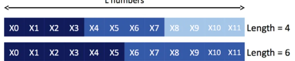
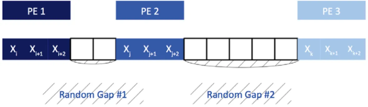
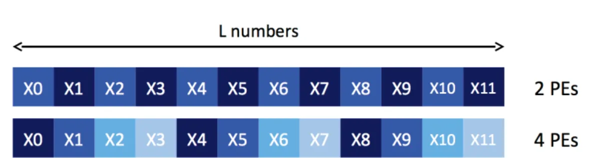
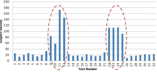
(18) List of Figures. 1.1. Floating-Point Operations per Second for the CPU and GPU (from [NVIDIA, 2011]) . . . . . . . . . . . . . . . . . . . . . . . . . . . . . .. 12. Example of a grid containing 6 blocks of 12 threads (4x3) (from [NVIDIA, 2011]) . . . . . . . . . . . . . . . . . . . . . . . . . . . . . . . . . . . .. 18. Sequence splitting in a unique original stream considering 2 processing elements (PEs), then 3 PEs . . . . . . . . . . . . . . . . . . . . . . . .. 30. 2.2. Random spacing applied to 3 processing elements (PEs) . . . . . . . . .. 31. 2.3. Leap frog in a unique original stream considering 2 processing elements (PEs), then 4 PEs . . . . . . . . . . . . . . . . . . . . . . . . . . . . . .. 33. 2.4. Example of Parameterization for 3 processing elements . . . . . . . . .. 34. 2.5. UML class diagram of a parameterized PRNG . . . . . . . . . . . . . .. 42. 2.6. Class Diagram for MTGP and its components . . . . . . . . . . . . . .. 43. 2.7. Overall arrangement of streams and substreams of MRG32k3a (from the expanded version of [L’Ecuyer et al., 2002a]) . . . . . . . . . . . . . . .. 45. Number of suspect results versus test numbers (extract displaying tests 1 through 32) . . . . . . . . . . . . . . . . . . . . . . . . . . . . . . . .. 56. 3.2. Detailed Results for Tests 35 and 100 of the BigCrush battery . . . . .. 57. 3.3. Extracts of the results for Test 35: MTGP identifiers versus random seeds indices . . . . . . . . . . . . . . . . . . . . . . . . . . . . . . . . .. 59. Percentage of passed results noticed for tests 35 and 100 depending on the PRNG . . . . . . . . . . . . . . . . . . . . . . . . . . . . . . . . . .. 60. 3.5. Bijective relation between threads and stochastic streams . . . . . . . .. 63. 3.6. Two random streams parallelizations based upon Sequence Splitting with two different sub-sequences lengths . . . . . . . . . . . . . . . . .. 64. 1.2. 2.1. 3.1. 3.4.

(19) xvi 3.7. List of Figures Random Spacing creation of three sub-sequences of equal length but differently spaced from each other . . . . . . . . . . . . . . . . . . . . .. 66. 3.8. Different threads numbers leading to different random substreams through the Leap Frog method . . . . . . . . . . . . . . . . . . . . . . . . . . . 66. 3.9. Simple representation of the major elements of a GPU . . . . . . . . .. 70. 3.10 PRNGs implementation scopes and their location in the different memory areas of a GPU . . . . . . . . . . . . . . . . . . . . . . . . . . . . .. 72. 3.11 Taxonomy of distribution techniques . . . . . . . . . . . . . . . . . . .. 75. 4.1. Parameterized Version of the Model . . . . . . . . . . . . . . . . . . . .. 84. 4.2. Meta-Model Describing the ShoveRand Framework . . . . . . . . . . .. 89. 4.3. UML class diagram of the expected interface of a PRNG in Shoverand. 96. 4.4. 3 Threads Jump Ahead Example . . . . . . . . . . . . . . . . . . . . . 105. 4.5. One worker thread per Processing Element is created. It is assigned a queue of tasks to process. . . . . . . . . . . . . . . . . . . . . . . . . . 107. 4.6. Substreams allotted to 3 different tasks and the corresponding pseudorandom sequence from the point of view of a sequential process . . . . 116. 5.1. Worm-like chain model of chromosomes . . . . . . . . . . . . . . . . . . 126. 5.2. A parallel rotation step for 3 blocks . . . . . . . . . . . . . . . . . . . . 129. 5.3. Example of generation of three possible futures for three different blocks 129. 5.4. Compatibility graph of the possible futures . . . . . . . . . . . . . . . . 133. 5.5. Cylindrical element that is part of the chromosome . . . . . . . . . . . 135. 5.6. Pseudo-cylindrical approximation of a segment . . . . . . . . . . . . . . 135. 5.7. Gnuplot 3D representation of a chromosome . . . . . . . . . . . . . . . 138. 5.8. Increase in the acceptance rate with the number of possible futures . . 139. 5.9. Improved performance of the model when run on a Kepler architecture K20 GPU . . . . . . . . . . . . . . . . . . . . . . . . . . . . . . . . . . 140.

(20) List of Figures. xvii. 5.10 Comparison of the execution times of 3 configurations of the Polymer Folding Model on 3 different GPUs . . . . . . . . . . . . . . . . . . . . 141 6.1. Output of the Netbeans Profiler after 200 iterations of the sequential Gap Model . . . . . . . . . . . . . . . . . . . . . . . . . . . . . . . . . 161. 6.2. Execution time for 10 different platforms running the simulation on a different map sizes . . . . . . . . . . . . . . . . . . . . . . . . . . . . . 163. 6.3. Schema showing the similarities between the two approaches: Scala Parallel Collections spread the workload among CPU threads (T), while ScalaCL spreads it among OpenCL Processing Elements (PEs) . . . . . 168. 6.4. Lattice updated in two times following a checkerboard approach . . . . 172. 6.5. Speed-up obtained for the Gap Model depending on the underlying technique of parallelization . . . . . . . . . . . . . . . . . . . . . . . . . . . 176. A.1 UML class diagram of the gap model . . . . . . . . . . . . . . . . . . . 207 A.2 Three different fall shapes for trees . . . . . . . . . . . . . . . . . . . . 208 A.3 Concentric light circles determine the amount of sunlight reaching the ground in windthrows . . . . . . . . . . . . . . . . . . . . . . . . . . . . 209 B.1 Representation of thread disabling to place the application at a warp-level214 B.2 Computation time versus number of replications for the Monte Carlo Pi approximation with 10,000,000 draws . . . . . . . . . . . . . . . . . . . 222 B.3 Computation time versus number of replications for a M/M/1 queue model with 10,000 clients . . . . . . . . . . . . . . . . . . . . . . . . . . 222 B.4 Computation time versus number of replications for a random walk model with 1,000 steps (above: 100 replications, below: 1,000 replications)224 B.5 Comparison of TLP and WLP ratio of the overall Global Memory access time versus computation time . . . . . . . . . . . . . . . . . . . . . . . 224.

(21)

(22) List of Tables 3.1. Summary of the potential PRNG/Parallelization technique associations. 68. 3.2. Summary of the potential uses of Distribution Techniques . . . . . . . .. 76. 4.1. Computation time of several sequential calls to the getTaskId() method 111. 4.2. BigCrush failed results for ThreadLocalRandom and TaskLocalRandom used by 16, 32 and 64 threads. Each test configuration was initialized with 60 different seed-statuses . . . . . . . . . . . . . . . . . . . . . . . 116. 4.3. Ability of Java PRNG facilities to deal with threads and tasks . . . . . 117. 6.1. Comparison of the studied APIs according to three criteria . . . . . . . 159. 6.2. Summary of the studied models’ characteristics . . . . . . . . . . . . . 169. 6.3. Characteristics of the three studied models . . . . . . . . . . . . . . . . 174. 6.4. Execution times in seconds of the three models on several parallel platforms (ScalaPC stands for Scala Parallel Collections) . . . . . . . . . . 175. B.1 Equivalence between original WLP through macros and aspect implementation . . . . . . . . . . . . . . . . . . . . . . . . . . . . . . . . . . 219 B.2 Number of read and write accesses to Global Memory for TLP and WLP versions of the Random Walk . . . . . . . . . . . . . . . . . . . . . . . 224.

(23)

(24) Listings 4.1. The interface of the policy is checked through Boost Concept Check Library . . . . . . . . . . . . . . . . . . . . . . . . . . . . . . . . . . . .. 87. 4.2. MTGP Integrated in ShoveRand . . . . . . . . . . . . . . . . . . . . . .. 90. 4.3. Example of use of the cuRand API . . . . . . . . . . . . . . . . . . . .. 92. 4.4. Example of use of the Thrust API . . . . . . . . . . . . . . . . . . . . .. 93. 4.5. Example of use of Shoverand . . . . . . . . . . . . . . . . . . . . . . . .. 94. 4.6. Example of use of ThreadLocalMRG32k3a . . . . . . . . . . . . . . . . 105. 4.7. Presentation of the API of TaskLocalRandom . . . . . . . . . . . . . . 113. 5.1. Calculation of collisions between spheres . . . . . . . . . . . . . . . . . 135. 5.2. Configuration of ShoveRand to use MRG32k3a . . . . . . . . . . . . . . 136. 5.3. Initialization of ShoveRand with the number of blocks to be used . . . 136. 5.4. Pseudorandom number drawn through ShoveRand . . . . . . . . . . . . 137. 6.1. GPU devices listing and kernel creation using the C++ wrapper API (adapted from [Scarpino, 2011]) . . . . . . . . . . . . . . . . . . . . . . 149. 6.2. GPU context creation kernel enqueueing using QtOpenCL . . . . . . . 151. 6.3. GPU program building using PyOpenCL . . . . . . . . . . . . . . . . . 152. 6.4. Computing cosine of the 1,000,000 first integers through ScalaCL . . . 153. 6.5. Squaring an array of integers using Aparapi . . . . . . . . . . . . . . . 154. 6.6. Squaring an array of integers using JavaCL . . . . . . . . . . . . . . . . 158. 6.7. Sequential version of method processLattice from class IsingModel . . . 172. 6.8. Parallel version of method processLattice from class IsingModel, using Scala Parallel Collections . . . . . . . . . . . . . . . . . . . . . . . . . . 173. B.1 Const-definition of warpIdx . . . . . . . . . . . . . . . . . . . . . . . . 215 B.2 Directive enabling warp-scope execution . . . . . . . . . . . . . . . . . 216.

(25) xxii. Listings. B.3 A whole WLP kernel . . . . . . . . . . . . . . . . . . . . . . . . . . . . 219 B.4 WLP on part of the code only . . . . . . . . . . . . . . . . . . . . . . . 220.

(26) List of Algorithms 5.1. Monte Carlo procedure involved in the simulation process . . . . . . . . 127.

(27)

(28) Introduction “Not so! Alas! Not so. It is only the beginning. — Bram Stoker, Dracula. Pseudorandom Numbers for Parallel Stochastic Simulations The need to reproduce runs of simulations forces the simulation community to champion PseudoRandom Number Generators (PRNGs) as a random source for their applications. However, this kind of random number generation algorithm is sensitive to the way its output random stream is partitioned among computational elements when used in parallel. Consequently, we need highly reliable Random Number Generators (RNGs) and sound partitioning techniques to feed such applications. From the practitioner point of view, sound partitioning techniques of stochastic streams must be employed in the domain of parallel stochastic simulations. Parallel and Distributed Simulation (PDS) is an area where extensive research of effective solutions has been developed. Deterministic communication protocols for synchronous and asynchronous simulation have been studied to avoid deadlocks and preserve causality and the principle of determinism. When considering stochastic simulations, the pseudorandom numbers must be generated in parallel, so that each Processing Element (PE) can autonomously obtain its own stream of pseudorandom numbers independent of other PEs. If independence is not established, the intrinsic statistical qualities are not guaranteed anymore, and the consequences are much more severe because the quality of the results can be flawed.. GPUs and the Emergence of Hybrid Computing for Simulation Recent developments sometimes use trillions of pseudorandom numbers necessitating the use of modern generators [Maigne et al., 2004]. In this context, the problem is that.

(29) 2. Introduction. the execution time of the simulation can be prohibitive without parallel computing. Lately, it has been possible to reduce the computation time of the heaviest simulations based on generalist graphics processors: the GP-GPUs (General Purpose Graphics Processing Units), also named GPUs for the sake of simplicity. These devices open up new possibilities for parallelization, but they also introduce new programming difficulties. Actually, GPUs behave as SIMD (Single Instruction, Multiple Data) vector processors. Such architectures are usually not very convenient to develop on for most developers as they are not familiar with the way they work. In order to democratize GPU programming among the parallel developers community, NVIDIA, the leading vendor of GPUs for scientific applications, has introduced a new programming language called CUDA (Compute Unified Device Architecture) [Kirk and Hwu, 2010]. CUDA exposes threads instead of vectors to developers. As a result, GPUs programming has become more similar to multithread programming on traditional CPUs. Still, there are still lots of constraints bound to GPUs, going from their particular memory hierarchy to thread scheduling on the hardware. Moreover, efficient developments must actually harness both CPU and GPU at the same time to balance the workload on the most appropriate architecture for a task. This paradigm is known as hybrid computing. All these parameters make it difficult for non-specialists to leverage the computing power of GPUs. In addition, they need to handle correctly the distribution of pseudorandom numbers on the device. Theoretical concerns regarding the use of pseudorandom numbers in parallel environments are known for a while and it is interesting to study how well they cope with recent parallel platforms, such as GPUs.. On the need for good software engineering practices CPU-enabled simulations can take advantage of a wide range of statistically sound PRNGs and libraries, but we still need quality random number generators for GPU architectures, and more precisely, a particular care has to be given to their parallelization. Many tries have been done to propose GPU-enabled implementations of PRNGs. Previous studies like [Bradley et al., 2011] bring up random number generation on GPU. Many strategies were adopted, but few of them perform well enough to distinguish themselves. It is also very difficult to select the right PRNG to use since both the statistical quality of the PRNG, and the quality of the GPU implementation need to.

(30) Introduction. 3. be considered for the overall performance of the application not to seriously drop. Recent development frameworks like CUDA enabled much more ambitious developments on GPU. We can now make use of some software engineering techniques, such as Object-Oriented programming or generic programming within GPU applications. This introduces a new scope in GPU-enabled applications development. As GPU-enabled software becomes more complex, it also needs enhanced tools to rely on. Thus, PRNGs implementations on GPU cannot be achieved in non-structured software development environments anymore. We need high-level software tools to smoothly integrate PRNGs in existing developments. In this thesis, we will also put software engineering considerations at the heart of our work and exploit successively Object-Oriented programming, generic programming and Aspect-Oriented programming to serve the needs of parallel stochastic simulation on GPUs and manycore architectures. On the one hand, these tools can fill the gap displayed by recent technologies such as GPU programming. We will present, for instance, an implementation based upon generic programming in C++ to overcome the lack of Object-Oriented features of old NVIDIA CUDA-enabled GPUs. On the other hand, techniques such as Aspect-Oriented programming will enhance existing tools and allow us to introduce extensions to the language without having to write a compiler or a Domain Specific Language (DSL) [Van Deursen et al., 2000]. Finally, Object-Oriented modelling and programming will be involved when it comes to interface with existing developments, or propose counterparts to standard libraries such as those issuing with the Java Development Toolkit.. Organization of the thesis This thesis studies the efforts that have to be made to port a parallel stochastic simulation on GPU, focusing on NVIDIA hardware and the associated CUDA technology. More particularly, it shows the need for good software engineering practices when taking care of pseudorandom numbers distribution across parallel platforms such as GPUs (Chapter 1). We will start by proposing a review of the current literature regarding Pseudorandom Number Generation in parallel and distributed environments. This will summarize the techniques employed to correctly distribute pseudorandom streams across Processing Elements (PEs), with a particular focus on GPUs (Chapter 2)..

(31) 4. Introduction. Having surveyed the behaviour of Pseudorandom Number Generators (PRNGs) in parallel environments, and particularly on GPU, we will propose theoretical guidelines to lead the design and implementation of these tools on GPU platforms. This advice takes into account the specificities of the architecture of GPUs, such as their memory hierarchy and thread scheduling (Chapter 3). Then, we will apply software engineering techniques to implement these theoretical guidelines on both GPU and manycore architectures. Our GPU-enabled development is a C++/CUDA library named ShoveRand that uses Template Metaprogramming to check design constraints at compile time. We target manycore architectures through Java task frameworks. To do so, we introduce TaskLocalRandom, a Java class that handles pseudorandom stream distribution across the tasks of a Java parallel application (Chapter 4). The presentation of a stochastic simulation model where some of these developments have been integrated will follow. Our main simulation application is a chromosome folding model entirely running on GPU. It is a first parallel version aiming at improving an initial sequential model which encounters troubles to evolve in some configurations (Chapter 5). We will eventually discuss a major issue when it comes to parallelize an application: choose the right parallel platform and programming languages. Our final chapter studies the possibility to automatically build prototypes of parallel applications targeting various platforms for free, with the help of software engineering tools from the literature. This strategy obviously needs to be combined with a good quality software toolchain, especially when it comes to Pseudorandom Number generation. Through this approach, the main input of this work about correct Pseudorandom Number distribution across parallel environments is reinforced (Chapter 6). We will now start by stating the context and problems studied in this thesis in Chapter 1..

(32) Chapter 1. Parallel Pseudorandom Numbers at the Era of GPUs: The Need for Good Software Engineering Practices. “[...] I estimate that even if fortune is the arbiter of half our actions, she still allows us to control the other half, or thereabouts. — Niccolò Machiavelli, Il Principe. Contents 1.1. Parallel Stochastic Simulation and Random Numbers . . . .. 6. 1.2. About Random Numbers . . . . . . . . . . . . . . . . . . . . . .. 7. 1.2.1. Pseudorandom Numbers . . . . . . . . . . . . . . . . . . . . . . .. 7. 1.2.2. Why do we settle for Pseudorandom Numbers when True Random Numbers are available? . . . . . . . . . . . . . . . . . . . . .. 7. 1.3. Pseudorandom Number Generation in parallel . . . . . . . . .. 10. 1.4. Pseudorandom streams on GPU . . . . . . . . . . . . . . . . .. 11. 1.5. Details about GPUs: programming and architecture . . . . .. 13. 1.6. 1.5.1. Architecture. . . . . . . . . . . . . . . . . . . . . . . . . . . . . .. 13. 1.5.2. Programming model of NVIDIA GPUs . . . . . . . . . . . . . . .. 16. 1.5.3. Programming languages . . . . . . . . . . . . . . . . . . . . . . .. 19. On the need for software engineering tools . . . . . . . . . . .. 22. 1.6.1. Software Engineering . . . . . . . . . . . . . . . . . . . . . . . . .. 22. 1.6.2. Object-Oriented Modelling . . . . . . . . . . . . . . . . . . . . .. 22. 1.6.3. Template MetaProgramming . . . . . . . . . . . . . . . . . . . .. 24.

(33) 6. 1.1. Chapter 1. Parallel Pseudorandom Numbers at the Era of GPUs. Parallel Stochastic Simulation and Random Numbers. Stochastic simulation is now an essential tool for many research domains. They can require a huge computational capacity particularly when we design experiments to explore large parameter spaces [Kleijnen, 1986]. New technologies in HPC and networking, including hybrid computing, have very significantly improved our computing capacities. The major consequence is the increased interest for parallel and distributed simulation [Fujimoto, 2000]. Random number generators (RNGs) are mainly used in simulation to model the stochastic phenomena that appear in the formulation of a problem or to apply an iterative simulation-based problem solving technique (such as Monte Carlo simulation [Gentle, 2003]) or coupling between simulation and Operations Research optimization tools. Reproducing experiments is the essence of science, and even if this is not always necessary, in the case of stochastic simulation, the need for reproducible generators is essential for various purposes, including the analysis of results. To investigate and understand the results, we have to reproduce the same scenarios and find the same confidence intervals every time we run the same stochastic experiment. When debugging parallel stochastic applications, we need to reproduce the same control flow and the same result to correct an anomalous behaviour. Reproducibility is also necessary for variance reduction techniques, for sensitivity analysis and many other statistical techniques [Kleijnen, 1986; L’Ecuyer, 2010]. In addition, for rigorous scientific applications, we want to obtain the same results if we run the application in parallel or sequentially. Consequently, software random number generation remains the prevailing method for HPC, and we will see that specialists are warning us to be particularly careful when dealing with parallel stochastic simulations [De Matteis and Pagnutti, 1990a; Pawlikowski and Yau, 1992; Hellekalek, 1998b; Pawlikowski and McNickle, 2001]..

(34) 1.2. About Random Numbers. 1.2 1.2.1. 7. About Random Numbers Pseudorandom Numbers. Pseudorandom Number Generators (PRNGs) use deterministic algorithms to produce sequences of random numbers and have been studied in pertinent reviews, many from Michael Mascagni and Pierre l’Ecuyer, and also from other authors, including the wellknown first edition of Knuth’s Art of Computer Programming, volume 2 and its reeditions [Knuth, 1969; James, 1990; L’Ecuyer et al., 2002a; Mascagni and Chi, 2004]. If some applications can cope with ’bad’ or poor randomness according to current standards, we cannot afford producing biased results for simulations in nuclear physics or medicine for instance [Li and Mascagni, 2003; Maigne et al., 2004; Lazaro et al., 2005; El Bitar et al., 2006; Reuillon, 2008a]. For parallel stochastic simulations, there is an even more critical need for a large number of parallel and independent random sequences [L’Ecuyer and Leydold, 2005], each with good statistical properties (approximating as close as possible a truly random sequence). We cannot give a mathematical proof of independence between two random sequences, so each time this word is used, it should be considered as (pseudo) independence according to the best accepted practices in mathematics and statistics. In mathematics, the notion of ‘pseudo’-random refers to polynomial-time unpredictability properties in the area of cryptology. However, in this thesis, we do not consider RNGs for cryptographic usage but only for scientific simulations. We do not consider quasi-random numbers either. They can improve the convergence speed (and accuracy) of Monte Carlo integration and also of some Markovian analysis [Niederreiter, 1992]. However, these numbers are not independent and even if they are interesting they can only be used for some specific applications.. 1.2.2. Why do we settle for Pseudorandom Numbers when True Random Numbers are available?. Before considering the use of True Random (TR) sequences in stochastic simulations, we need to recall the basic principles of such applications. Stochastic simulations are developed for their results to be analysed and reproducible. To do so, we need to master every parameter of the model. Considering stochastic models, the random sequence.

(35) 8. Chapter 1. Parallel Pseudorandom Numbers at the Era of GPUs. feeding the simulation is also a parameter that we need to be able to reuse and provide to other scientists. In doing so, they can check or rerun our experiments and check the results. As long as True Random sequences are not issued by a deterministic algorithm but by quantum phenomena, they are not reproducible if they are not stored. This supposes that True Random sequences in Stochastic Simulations would have to be prerecorded in files before being used. This is perfectly suitable for small scale simulations where memory mapping techniques will help to reduce the impact on performances (see [Hill, 2003] for more details about unrolling of random sequences). However, this approach has the major drawback that the files containing the TR numbers will have to be located on the same machine as the simulations programs they feed. In order to explore a Design of Experiments (DOE), or to run several replications of a High Performance Simulation (MRIP: Multiple Replications in Parallel), we will often want to distribute these independent executions in order to speed-up the whole experiment time. This raises the problem of the random data migration. For more than 7 years, our research team has been faced with simulations in nuclear physics and medicine that needed up to hundreds of billions of random numbers (for a single replicate). This represents tenths of gigabytes. As a matter of fact, moving such amounts of data to distributed environments, such as computing grids for instance, might significantly impact the overall execution time of the simulation. Now, we can think of other approaches. Being not reproducible is not the sole constraint of True Random sequences. Most of the time, their numbers are generated with the help of either internal or external devices plugged into a computer. These devices may vary from a small USB key to recent GPU boards. Consequently, if we want to take advantage of True Random features in a distributed environment, we must ensure that every machine that will run our binaries is equipped with such devices. Unfortunately, this is hardly possible when we consider serious distributed systems where resources are shared by a large community across a wide area. For example, as users of the European Grid Initiative (EGI), we are not aware of any True Random equipment available in EGI’s sites (among more than 337,000 cores available at the time of writing). Lastly, we could rely on a central element to provide random numbers in a distributed environment. This would imply having one or several servers, dedicated to True Random numbers generation across a network. Moreover, we would also need a user-friendly API (Application Programming Interface) allowing one to easily get random numbers from these servers. The web site located at http://random.irb.hr/ offers such a service [Stevanovic et al., 2008], but only for very low scale applications..

(36) 1.2. About Random Numbers. 9. Registered users benefit from an easy to use library to get True Random numbers directly from a remote server. Basically, centralized approaches are well-known for the bottleneck problem they introduce. Apart from this previously evoked problem, which makes a central server hardly implementable in a High Performance Computing context, the ‘irb’ library displays other weaknesses. First, it is based upon the network availability of the server, which might not be a 100% reliable way to draw random numbers. Moreover, what appears as an attempt to prevent bottlenecks becomes a hindrance: there are quotas limiting the daily numbers output to 100 MB per user, with respect of a monthly barrier of 1GB per user. This does not meet at all HPC expectancies. Finally, we have described three ways to employ TR numbers within stochastic simulations: • Take advantage of a device plugged in the machine running the simulation; • Record True Random sequences in files; • Query a remote server for the numbers. These approaches have all displayed major flaws, and are clearly not satisfying solutions in an HPC environment executing a large amount of simulations. As a conclusion, we still have to champion Pseudorandom Numbers Generators, whose statistical quality is good enough for any scientific application nowadays. Pseudorandom Numbers Generators are a definitely more portable solution when tackling distributed applications. The portability of PRNGs usually results from the few hundred lines of code necessary to implement them. Although True-Random numbers would bring a perfectly unpredictable randomness, only sensitive cryptographic applications require this characteristic. On the other hand, scientific applications might even take advantage of the deterministic behaviour of PRNGs. At the time of writing, True Random numbers sequences are not a relevant solution neither for HPC nor for stochastic simulation because of hardware considerations. However this might evolve in the future in view of an innovative Intel chip, called Bull Mountain, which takes advantage of True Random number generation facilities. This chip is already integrated in the cutting-edge Intel’s Ivy Bridge architecture, but at the moment the TRNG is so slow that it is dedicated to seed a hardware-implemented PRNG..

(37) 10. 1.3. Chapter 1. Parallel Pseudorandom Numbers at the Era of GPUs. Pseudorandom Number Generation in parallel. When dealing with stochastic parallel simulation, we have to consider two main aspects: the quality of the PRNG and the technique used to distribute pseudorandom streams across parallel Processing Elements (PE). If stochastic sequential simulations always require a statistically sound PRNG, in the case of parallel simulations, this requirement is even more crucial. The parallelization technique should ideally generate pseudorandom numbers in parallel, that is, each PE should autonomously obtain either its own pseudorandom sequence or its own subsequence of a global sequence (partitioning of a main sequence). If such independence is not guaranteed, the parallelism is affected. Then, the sequences assigned to each PE must not depend on the number of processors, or the simulation results could not be reproduced. Designers of parallel stochastic simulations always have to reply to this fundamental question: how can we make a safe RNG repartition to keep, on the one hand, efficiency, and on the other hand, a sound statistical quality of the simulation to obtain credible results? Indeed, the validation of such parallel simulations is a critical issue. Paul Coddington precisely states: ‘Random number generators, particularly for parallel computers, should not be trusted’ [Coddington and Ko, 1998]. Much research has been undertaken to design good sequential RNGs. Whatever the parallelization technique is, we have to rely on a ‘good’ sequential generator according to a set of main principles proposed by specialists [Lagarias, 1993; Coddington and Ko, 1998; Hellekalek, 1998a]. Among the best generators currently available, we can cite Mersenne Twister (MT hereafter) [Matsumoto and Nishimura, 1998] introduced in 1997. SFMT [Saito and Matsumoto, 2008] is currently less known. It is an SIMD-oriented version of the original Mersenne Twister generator with the following improvements: speed (twice as fast as MT), a better equidistribution and a quicker recovery from bad initialization (zero-excess in the initial state). The periods being supported by SFMT are incredibly large, ranging from 2607 to 2216091 . The WELL generators (Well Equidistributed Long-period Linear), on the basis of similar principles (Generalized Feedback Shift Register), have been produced by Panneton in collaboration with L’Ecuyer and Matsumoto [Panneton, 2004]. L’Ecuyer suggests that multiple recurrence generators (MRGs) with much smaller periods (above 2100 but less than 2200 ), such as MRG32k3a [L’Ecuyer and Buist, 2005], can also have very interesting statistical properties, and are easier to parallelize according to our current knowledge. At the end of the 1980s, as the interest for distributed simulation increased, numerous research works took on to.

(38) 1.4. Pseudorandom streams on GPU. 11. design parallel RNGs [De Matteis and Pagnutti, 1988; Durst, 1989; Percus and Kalos, 1989; Eddy, 1990; De Matteis and Pagnutti, 1995; Entacher et al., 1999; Srinivasan et al., 2003]. Assessing the quality of random streams remains a hard problem, and many widely used partition techniques have been shown to be inadequate for some specific applications. For instance, several studies in networking and telecommunication question the relevance of many stochastic simulations because of the use of poor quality RNGs [Pawlikowski and Yau, 1992; Pawlikowski, 2003b; Hechenleitner, 2004], as well as the mediocre parallelization techniques used in some software [Entacher and Hechenleitner, 2003]. Chapter 2.3 will give a survey of those parallelization techniques.. 1.4. Pseudorandom streams on GPU. Recent developments try to shrink computation time by relying more and more on Graphics Processing Units (GPUs) to speed-up stochastic simulations. Such devices bring new parallelization possibilities thanks to their high computing throughput compared to CPUs, as explained by Figure 1.1. They also introduce new programming difficulties. Since the introduction of Tesla boards, Nvidia, ATI and other manufacturers of GPUs have changed the way we use our high computing performance resources. Since 2010, we have seen that the top supercomputers are now often hybrid. Given that RNGs are at the base of any stochastic simulation, they also need to be ported to GPU. In this thesis we intend to present the good practices when dealing with pseudorandom streams on parallel platforms, and especially on GPUs. Two main questions arise from these considerations: • How are these random streams produced on GPU? • How can we ensure that they are independent? In our case, we focus on the parallelization techniques of pseudorandom streams used to directly feed parallel simulation programs running on GPU (called kernels in the CUDA language). Before stating what we will study in this thesis, let us point out first, that we will not propose any new PRNG, and second, that our study is not tied to the parallelization of random number generation algorithms, albeit we do survey some parallel PRNG algorithms. Still, Chapter 3.3 proposes guidelines that will hopefully help developers to use reliable parallelization techniques of random streams to.

(39) 12. Chapter 1. Parallel Pseudorandom Numbers at the Era of GPUs. Figure 1.1: Floating-Point Operations per Second for the CPU and GPU (from [NVIDIA, 2011]) ensure their independence, and that are, in addition, well adapted to GPU architectures particularities. Some works have attempted to speed-up generation using the GPU before retrieving random numbers back onto the host. However, current CPU-running PRNGs display fairly good performances thanks to dedicated compiler optimizations. For instance, Mersenne Twister for Graphics Processors (MTGP) [Saito and Matsumoto, 2013], the recent GPU implementation of the well-known Mersenne Twister [Matsumoto and Nishimura, 1998], is announced as being 6 times faster than the CPU reference SFMT (SIMD-oriented Fast Mersenne Twister) [Saito and Matsumoto, 2008], which is already very efficient in terms of performance. Meanwhile, previous studies have shown that the time spent generating pseudorandom numbers could represent at most 30% of CPU time for some “stochastic-intensive” nuclear simulations [Maigne et al., 2004], but they are very scarce. For less intensive simulations, where less than a billion numbers are needed, there is no real need for parallelization and unrolling is still the most efficient technique [Hill, 2003]. Considering the small part of the execution time used by most stochastic simulations to generate random numbers, it is not worth limiting GPUs usage at the generation task. To har-.

(40) 1.5. Details about GPUs: programming and architecture. 13. ness the full potential of GPUs, we are more interested in providing random numbers to GPU-running applications that will consume them directly on the device.. 1.5. Details about GPUs: programming and architecture. In this section we will briefly introduce some background about NVIDIA GPUs on which this thesis mainly relies. We will describe in turn the architecture, the programming model and languages available to program such devices. Although this section focuses on NVIDIA GPUs only, most of the notions introduced hereafter can apply to other brands of devices.. 1.5.1. Architecture. 1.5.1.1. Architecture of GPUs (before 2010): the example of the Tesla C1060 (T10) board. The Tesla C1060 card with the NVIDIA T10 processor was the first GPU dedicated to scientific computing. It does not even have a graphical output! GPUs were originally designed to perform relatively simple, but also very repetitive, operations for a large number of data (each pixel of an image for instance). They dedicate a wide area of their chip to processing units which can perform the same operation in parallel [Nickolls and Dally, 2010]. For example, while the majority of recent microprocessors have less than 10 cores, NVIDIA announced its Tesla T10 as owning 240 “CUDA cores”. However, the cores present in GPU and CPU cores are very different and it is not simple to take advantage of the enormous power of GPU. The core architecture of GPUs from Tesla T10 generation consists of 30 Streaming Multiprocessors (SMs) (3 in each of the 10 TPC - Thread Processor Clusters). Each of these streaming processors consists of several components: • for calculation: – 8 thread processors (SP Thread Processor or SP) for floating-point computations;.

(41) 14. Chapter 1. Parallel Pseudorandom Numbers at the Era of GPUs – 2 Special Function Units (SFU) performing complex mathematical calculations such as cosine, sine or square root; – 1 Double Precision unit (DP) for double-precision floating-point computations; • for memory management: – Shared Memory; – Cache.. The 240 “CUDA cores” announced by NVIDIA correspond to 240 (30x8) thread processors on the board. However, this is more a marketing denomination than an actual description. The element of a GPU that matches most of the characteristics of a CPU core are SMs. They have their own memory, cache and particularly scheduler. Thus, two distinct Streaming Multiprocessors can perform different instructions at the same time, whereas the thread processors belonging to the same SM cannot. Thread processors behave according to the SIMD (Single Instruction Multiple Data) paradigm, executing a single statement on 8 different data sets only. Moreover, unlike microprocessors, few efforts have been made over legacy GPUs to speed up memory accesses, making them particularly disadvantageous for an application.. 1.5.1.2. GPU Architecture (2010-2012): the inputs of Fermi. The second architecture of NVIDIA GPUs, codenamed Fermi, corrects the main limitations mentioned above and improves the raw performance. The declination of this GPU architecture dedicated to scientific computing is the Tesla C2075. In terms of computing power, the C2075 has only 14 streaming multiprocessors, compared to the 30 SMs of the previous C1060. They are composed of two groups - scheduled separately – of 32 SIMD thread processors (448 "CUDA cores" versus 240 previously). In addition, double precision floating point calculations on these thread processors support the IEEE754-2008 standard. The double precision calculations have been significantly improved: each SM now owns 1 double-precision unit for 2 single-precision units, whereas the previous ratio was 1 double-precision unit for 8 single-precision units [Wittenbrink et al., 2011]. The major changes brought by this new architecture is the appearance of L1 and L2 caches. The 64KB L1 cache is also used to implement the shared memory area of the SM. It is partly configurable as it allows allocating the largest part (48KB) to.

(42) 1.5. Details about GPUs: programming and architecture. 15. either L1 cache or shared memory. The appearance of these caches usually helps to increase the performance of an application for free. With regard to reliability, Fermi introduces a major input with ECC (Error Correcting Code) RAM available with the scientific range of NVIDIA GPUs. This is mandatory for HPC applications on the road to exascale computing, where lots of physical parameters (alpha particles, . . . ) can occasionally modify data in memory. Finally, the architecture, coupled with a version of the CUDA SDK from 4.0 and later, improves compatibility with the C++ standard. It proposes the main features of C++ on the device: dynamic allocation, inheritance, polymorphism, templates, . . .. 1.5.1.3. GPU Architecture (> 2012): Kepler. The new architecture proposed by NVIDIA in late 2012 was named Kepler [NVIDIA, 2012]. The Kepler architecture continues to improve the performance of GPU computing while focusing on a more economical power consumption. The number of CUDA cores continues to increase, rising from 240 CUDA cores for the C1060 to 448 cores for the C2050, and now 2,496 cores for the K20, the scientific version of the Kepler generation. However, let us recall that these CUDA cores are nothing more than vector units and should not be compared to traditional CPU cores. The two major features of this architecture are called Dynamic Parallelism and Hyper-Q. Dynamic Parallelism can break the master-slave relationship between the CPU and the GPU. Traditionally, the CPU controls the execution and delegates massively parallel computing to the GPU. Dynamic Parallelism allows the GPU to gain autonomy in being able to launch new parallel computations without CPU intervention. The other novelty, Hyper-Q, focuses on a problem tied to the popularization of GPUs. Many developments including GPU cannot take advantage of 100% of their capacity. To compensate this under-utilization, Hyper-Q allows multiple CPUs to address the same GPU. Previously, only one physical connection was possible between CPU and GPU. Now, up to 32 connections can be created. Several applications could also benefit from this new opportunity. We think primarily of applications using MPI to distribute the workload across multiple CPU cores, which can now collaborate with each GPU installed in the host machine. Dynamic Parallelism and Hyper-Q are only enabled on Kepler devices which host runs a CUDA 5.0 SDK..

(43) 16. Chapter 1. Parallel Pseudorandom Numbers at the Era of GPUs. 1.5.1.4. Summary. The main advantage of GPUs is obviously the potential computing capacity that this technology offers at low cost. At the time of writing, parallel applications running on GPUs are still strongly impacted by the poor performance of some memory accesses within the same GPU and memory transfers between the CPU and the GPU. Even if recent architectures have greatly improved things by adding caches, it is always necessary to perform the largest number of instructions on the smallest amount of data by computing element, in order to obtain the announced performances.. 1.5.2. Programming model of NVIDIA GPUs. NVIDIA call their parallel programming model SIMT (Single Instruction, Multiple Threads) [NVIDIA, 2011]. It is actually an abstraction layer of SIMD (Single Instruction, Multiple Data) parallel architectures described in Flynn’s taxonomy [Flynn, 1966]. The idea behind SIMT is to ease the use of a SIMD architecture to developers that are more used to create threads than to fill in vectors. The following lines will detail the base concepts of the SIMT programming model and its interaction with the hardware.. 1.5.2.1. Grids, Blocks and Threads. To take advantage of the many thread-processors present on the GPU, it is not necessary to manually create as many threads as desired and then assign each thread to a processor. Simply, the number of threads is specified when the function intended to run on the GPUs is called (named kernel in CUDA terminology). This number is provided by filling the block size (the number of threads included in a block) and the grid size (number of blocks included in the grid). To allow a large number of threads to run the same kernel, the threads must be grouped into blocks, which are grouped in a grid. The distribution between the grid and the blocks is left free to developers. These figures can significantly impact the performance of the parallel application. The two concepts of grid and blocks will be detailed later, it is sufficient for now to understand that a block contains a given number of threads and the grid contains a given number of blocks. Before coming to the very important concept of blocks, it is necessary to make a short digression on the concept of warp introduced by NVIDIA. A warp is a software.

(44) 1.5. Details about GPUs: programming and architecture. 17. concept that refers to a group of 32 threads that will execute the same instruction at the same time on a Streaming Multiprocessor (SM). The fact that it is a software concept means that there is no material equivalent to warps. The concept of warp has an important impact on the programming of GPUs because of their role in memory access and in thread scheduling. Actually, the memory accesses within a warp can be merged. Thus, if all the threads in a warp access contiguous memory locations, only two requests will be required. In addition, versions of pre-Fermi GPUs cannot schedule more than 48 warps at the same time on a single SM. A warp itself containing 32 threads, it is impossible to exceed 1,536 threads run simultaneously. Blocks are used to group the threads in a first logical group. Unlike warps, block can be controlled and configured by the developer. The maximum number of threads that can be contained in a block depends on the GPU board used (up to 1,024 threads per block on current GPU at the time of writing). The execution of all the threads belonging to the same block will be performed on a the same SM (conversely, threads present on different blocks can be executed on different SMs). Now being run on the same SM is not insignificant and will allow threads of the same block to take advantage of the shared memory area of the SM (to communicate but also to pool the memory accesses). It will also be possible to synchronize all the threads of a block at a specific location of a kernel. The sole utilization of blocks does not maximize the power of GPUs. They can run multiple blocks at the same time and thus increase the number of calculations in parallel. It is then necessary to have a large number of threads, a number that can easily happen to exceed the maximum of 1,024 threads in a block. In this case, it is necessary to work with multiple blocks in the grid. The grid represents the top bundle of threads launched for a given kernel. Historically, a single grid was associated with a kernel, but recent versions of CUDA (5.0 and later) now allow to launch new kernels, and thus create new grids, from a kernel. Figure 1.2 sums up the multi-scale hierarchy of threads at the heart of the SIMT programming model.. 1.5.2.2. Scheduling on the GPU. Most of the considerations in this section are from our personal experience, intersected with a smattering of documentation provided by NVIDIA on the subject. Although the CUDA language is well documented, the proprietary architecture that executes it often appears as a black box. This is particularly the case for GigaThread, the scheduler discussed in this section, whose behaviour may seem quite erratic at first..

(45) 18. Chapter 1. Parallel Pseudorandom Numbers at the Era of GPUs. Figure 1.2: Example of a grid containing 6 blocks of 12 threads (4x3) (from [NVIDIA, 2011]). A Streaming Multiprocessor (SM) of the Fermi architecture is composed of 32 thread-processors. Now, the SM works on warps with 32 threads. A SM is able to perform an operation for 32 threads of a warp at each clock tick. At the same time, warps are scheduled by two warp schedulers on each SM. Each warp scheduler, however, can only assign threads to half of the thread-processors, 16 threads in a single warp. Thus, it takes 2 clock cycles to fully execute an instruction for a warp. Moreover, thread-processors perform operations on data in memory that it is obviously necessary to load first. These memory accesses required to execute an instruction by an entire warp are made by warp (32 memory accesses at a time) on recent architectures, unlike the half-warp access of the previous architectures. Of course, the instructions can not be executed until data has been loaded and the performance decreases if no warp is ready to run. One key to achieve satisfactory performance on GPU is handling a large number of warps to hide latency. It is customary that the Fermi architecture requires a minimum of 18 per SM warps to hide latency for example. Thus, warp scheduling is necessary in order to hide at most the latency of memory accesses..

(46) 1.5. Details about GPUs: programming and architecture. 19. Another scheduling level takes place with blocks. A GPU owns several SMs, and it is possible to run several blocks simultaneously on different SMs. Scheduling is required when the number of blocks is too large to allow their simultaneous executions. In this case, the blocks are executed in several runs. The GPU can schedule up to 8 different blocks on a single SM, provided the limit of the maximum number of threads that can be scheduled on a SM is not reached at the same time. Blocks scheduling allows to some extent to reduce the impact of memory access by running other threads when some are awaiting data from the memory. Since each SM has its own unit to read and decode instructions, each block can be managed independently. Thus, a block which all threads have completely finished their execution can be immediately replaced by a new block without having to wait for all the blocks already assigned to the SM to complete. This mechanism explains why, in some cases, the execution time will slightly change when the number of blocks used is increased: as block execution can still be performed simultaneously, the total execution time does not increase in proportion to the number of threads used (although it generally grows, as increasing the number of threads usually leads to a rise in the size of the data to process, and thus of the number of memory accesses).. 1.5.3. Programming languages. 1.5.3.1. CUDA. The NVIDIA’s CUDA technology1 is the toolkit designed to exploit highly parallel computation using NVIDIA GPUs. Its SDK was first released by NVIDIA in February 2007. The main purpose of CUDA is to let people use GPUs as platforms for computations and not only for games. CUDA not only refers to a particular range of GPU architectures, but it also designates the tools and the language used to program the GPU. NVIDIA offers a lot of tools to code, debug and profile their applications, to developers willing to use their devices. The CUDA language provides an extension to the C++ language to allow interface with the GPU. All the constructs available in C++ are available in CUDA, but extra keywords and new functions are provided to communicate with the GPU, and parallelize the application. Even if NVIDIA releases a C++ SDK, wrappers exist that enable other languages 1. CUDA Zone: http://www.nvidia.com/object/CUDA_home_new.html, last access 8/12/13.