HAL Id: hal-00112620
https://hal.archives-ouvertes.fr/hal-00112620
Submitted on 9 Nov 2006
HAL is a multi-disciplinary open access archive for the deposit and dissemination of sci-entific research documents, whether they are pub-lished or not. The documents may come from teaching and research institutions in France or
L’archive ouverte pluridisciplinaire HAL, est destinée au dépôt et à la diffusion de documents scientifiques de niveau recherche, publiés ou non, émanant des établissements d’enseignement et de recherche français ou étrangers, des laboratoires
Ordered monoids and J-trivial monoids
Karsten Henckell, Jean-Eric Pin
To cite this version:
Karsten Henckell, Jean-Eric Pin. Ordered monoids and J-trivial monoids. J.-C. Birget, S. Margolis, J. Meakin and M. Sapir. Algorithmic problems in Groups and Semigroups (Lincoln, NE, 1998), Birkhäusern, Boston, MA, USA, pp.121-137, 2000, Trends in Mathematics. �hal-00112620�
Ordered monoids and
J -trivial monoids
Karsten Henckell∗and Jean-Eric Pin† July 19, 1999
Abstract
In this paper we give a new proof of the following result of Straubing and Th´erien: every J -trivial monoid is a quotient of an ordered monoid satisfying the identity x ≤ 1.
We will assume in this paper that the reader has a basic background in finite semigroup theory (in particular, Green’s relations and identities defining varieties) and in computer science (languages, trees, heaps). All semigroups except free monoids and free semigroups are assumed finite. As a consequence, the term variety always means variety of finite semigroups (or pseudo-variety) and the term identity refers to pseudo-identity, in the terminology of Almeida [2].
A relation ≤ on a semigroup S is stable if, for every x, y, z ∈ S, x ≤ y implies xz ≤ yz and zx ≤ zy. An ordered semigroup is a semigroup S equipped with a stable partial order ≤ on S. Ordered monoids are defined analogously.
Let A∗ be a free monoid. Given a subset P of A∗, the relation ¹P defined
on A∗ by setting u ¹P v if and only if, for every x, y ∈ A∗,
xvy ∈ P ⇒ xuy ∈ P,
is a stable partial preorder. The equivalence relation ∼P associated with
¹P is defined, for every x, y ∈ A∗, by
xuy ∈ P ⇐⇒ xvy ∈ P
The monoid M (P ) = A∗/∼P, ordered with the order relation induced by
¹P, is called the ordered syntactic monoid of P .
∗
New College of the University of South Florida, Sarasota, FL 34243, USA, [email protected]
†
LIAFA, Universit´e Paris VII et CNRS, Tour 55-56, 2 Place Jussieu, 75251 Paris Cedex 05, FRANCE, [email protected]
1.
Introduction
The aim of this paper is to give a new proof of the following result of Straub-ing and Th´erien [20]:
Theorem 1.1. Every J -trivial monoid is a quotient of an ordered monoid satisfying the identity x ≤ 1.
There are several reasons to consider Theorem 1.1 as an important result in the theory of finite semigroups. The first reason is its close connection with a celebrated result of Simon in language theory [16]. Recall that a language of A∗is piecewise testable if it is a boolean combination of languages of the form A∗a1A∗a2A∗· · · A∗anA∗. Simon’s theorem can be stated as
follows.
Theorem 1.2. A recognizable language is piecewise testable if and only if its syntactic monoid is J -trivial.
It is not very difficult to establish the equivalence of Theorems 1.1 and 1.2. In one direction, it suffices to observe that the ordered syntactic monoid of a language of the form A∗a1A∗a2A∗· · · A∗anA∗satisfies the identity x ≤ 1.
In the opposite direction, it is easy to establish that any language recognized by an ordered monoid satisfying the identity x ≤ 1 is piecewise testable. There are actually several known proofs of Theorem 1.2, but the proof of Straubing and Th´erien was the first to proceed by induction on the size of the monoid.
The second reason of the importance of Theorem 1.1 lies in the role played by ordered monoids in this statement. A systematic use of ordered monoids in language theory was initiated in [11] and developed for instance in [13, 14, 15]. This approach, combined with some deep results obtained in the recent years [3, 4, 5, 6, 7, 8, 9, 10] gives evidence that Theorem 1.1, far from being an isolated result, is actually the prototype of a new kind of covering theorems. We list a few of these results from [13] below, to give the flavor to the reader. Recall that a block group is a monoid in which every regular R-class and L-class contains a unique idempotent. Many equivalent definitions can be found for instance in [12].
Theorem 1.3. Every block group monoid is the quotient of an ordered monoid satisfying the identity xω ≤ 1.
Theorem 1.4. Every monoid with commuting idempotents is the quotient of an ordered monoid with commuting idempotents satisfying the identity xω ≤ 1.
Our last example comes from language theory. The languages of level 1 in the so called dot-depth hierarchy were characterized by Knast [9, 10]. Their syntactic semigroup satisfies Knast identity:
(xωpyωqxω)ωpyωs(xωryωsxω)ω = (xωpyωqxω)ω(xωryωsxω)ω (K) Theorem 1.5. Every semigroup satisfying (K) is the quotient of an ordered semigroup satisfying the identity xωyxω ≤ xω.
All these statements follow the same pattern, stated here in the monoid case:
Every monoid M of a certain variety of monoids V is the quotient of an ordered monoid ˆM of a certain variety of ordered monoids V0. Unfortunately, no direct proof of Theorems 1.3, 1.4 or 1.5 is known and it is a challenging problem to find such a direct proof. One of the difficulties is that the covering monoid ˆM is usually not constructed directly. Even in the proof of Straubing and Th´erien [20], the cover is built by induction on the size of M , and thus its construction requires several steps.
In this paper, we give a proof of Theorem 1.1 which provides a direct construction of the covering monoid. Although our construction is rather abstract, we hope it will be easier to adapt to the cases noted above than the indirect proofs.
Factorization forests play an important role in this proof. This gives some evidence that this concept introduced by Simon in 1989 [17, 18, 19] to supersede the Ramsey-type arguments used in semigroup theory, is indeed a fundamental tool. Another illustration of the power of factorization forests can be found in [13].
Technically speaking, our proof is a global version of that of Straubing and Th´erien. We keep the idea of using 2-factorizations, but since we want a direct construction, the induction used in [20] has to be done in one single step. This leads naturally to factorization trees, which exactly encode iter-ated factorizations. The level of induction of the Straubing-Th´erien proof is now controlled by the label of the nodes in the factorization tree. This is the reason why our factorizations trees form a heap with respect to the ≤J-order.
The resulting proof is certainly much longer than the original proof. The main reason is that dealing with trees requires an important amount of notation. Nevertheless, our construction is not conceptually difficult. Given a set of generators A of M , it consists in defining a preorder on A∗ in the following way:
(1) Every word admits a factorization tree.
(2) The ≤J-order on M induces a natural preorder ≤ on factorization
trees.
(3) The preorder on trees extends naturally to a preorder on words: if u and v are words, u ≤ v if, for every factorization tree s of u, there is a factorization tree t of v such that s ≤ t.
Now the equivalence ∼ associated with ≤ is a congruence of finite index, and the required cover is the monoid A∗/∼, equipped with the partial order inherited from ≤.
2.
Ordered monoids and
J -trivial monoids
In the sequel, we fix a J -trivial monoid M . Then there exists a finite alphabet A and a surjective monoid morphism π : A∗ → M such that, for each a ∈ A, µ(a) 6= 1. One can take for instance A = M \ {1} and set µ(a) = a for each a ∈ A.
The set of idempotents of M is denoted by E(M ) and the set of words of A∗ with an idempotent image in M is denoted by R. In particular, R = π−1(E(M )). An element which is not idempotent is called null. The
set of null elements of M is denoted by Null(M ). Finally, we denote by B = A \ R the set of letters with a null image in M . We first recall some elementary facts about J -trivial monoids.
Proposition 2.1. Let a, b, c ∈ M and e ∈ E(M ).
(1) If a ≤J b and if ac ∈ E(M ), then ac ≤Lbc (and thus ac ≤J bc).
(2) If e ≤J a, then e = ea = ae.
(3) If e ≤J a and e ≤J b, then e ≤J ab.
(4) If e ≤J abc, then e ≤J ac.
Proof. (1) If a ≤J b, then a = xby for some x, y ∈ M . Thus xbyc =
ac = (ac)(ac) = (xbyc)(xbyc). Since M is J -trivial, it follows that xbyc is fixed under right multiplication by x, b, y and c. Therefore ac = xbycxbc = (xbycx)bc. Thus ac ≤Lbc.
(2) If e ≤J a, e = xay for some x, y ∈ M . Thus xay = (xay)(xay)
and xay is fixed under right multiplication by a, whence e = ea. A dual argument would show that e = ae.
(3) If e ≤J a and e ≤J b, then ea = e = eb by (2) and thus e = eab,
whence e ≤J ab.
(4) If e ≤J abc, then e ≤J a since abc ≤J a. Similarly, e ≤J c, and by
(3), e ≤J ac.
We now introduce one of the key concept of this article. A good factorization of a word u ∈ A∗ is a triple of one of the following types:
(1) (u0, a, u1) with u0, u1 ∈ A∗, a ∈ B, u = u0au1, π(u) <J π(u0) and
π(u) <J π(u1).
(2) (u0, 1, u1) with u0, u1 ∈ A∗, u = u0u1, π(u) <J π(u0) and π(u) <J
π(u1).
Proposition 2.2. Every word of A∗\ R has a good factorization.
Proof. Let u ∈ A∗\ R. Since π(u) is not idempotent, u is not the empty
word, and π(u) <J π(1). Therefore, u has a maximal prefix u0 such that
π(u) <J π(u0). Setting u = u0au1, with a ∈ A, we have π(u0a) = π(u)
by the maximality of u0. It follows that π(u1) 6= π(u), for otherwise, π(u)
would be idempotent. Thus π(u) <J π(u1). If a ∈ B, (u0, a, u1) is a
good factorization of u. Otherwise π(a) is idempotent, and we claim that (u0, 1, au1) is a good factorization. We already know that π(u) <J π(u0)
and it suffices to verify that π(u) <J π(au1). Assume by contradiction that
π(u) = π(au1). Then, the sequence of equalities
π(u) = π(u0)π(a)π(u1) = π(u0)π(a)π(a)π(u1) = π(u0a)π(au1) = π(u)π(u)
shows that π(u) is idempotent, a contradiction.
3.
Binary trees
Binary trees play a crucial role in this article and we need a rigorous defi-nition of these objects. In general, given a set S of symbols and a set V of variables, the set T (S, V ) of binary trees over S and V is the smallest set T such that
(1) for each v ∈ V , (v) ∈ T ,
A set of trees is called a forest. The root, the leaves and the internal nodes of a tree t are defined by structural induction as follows.
(1) if t = (v), then v is the root and the unique leaf of t. In this case, t does not have any internal node.
(2) if t = (t0, s, t1), then s is the root of t. The leaves of t are those of t0
and of t1. The internal nodes of t are s and those of t0 and of t1.
It is often convenient to use a graphical representation for trees, according to the following rules:
(1) the tree (v) is represented by v ,
(2) if t0 and t1 are represented respectively by t0 and t1 , then
(t0, a, t1) is represented by a
t0 t1
In this representation, the leaves are variables and the internal nodes are symbols. For instance, the tree ((u, a, v), 1, ((v, a, v), b, (u, 1, w))) is repre-sented by 1 a u v b a v v 1 u w Figure 3.1. A tree
An occurrence of a node within a tree may be given by its position, which is a word of {0, 1}∗ describing the path from the root of the tree to the node, with the convention that 0 means left and 1 means right. For instance, in the tree represented in Figure 3., there are two occurrences of the node u, the nodes in position 00 and 110. Given a position p in a tree t, the subtree of t rooted at p is denoted t|p. The tree obtained by replacing this subtree t|p by a tree s is denoted by t[s]p. Here is the formal definition:
(2) If p = 0q for some q ∈ {0, 1}∗, and if t = (t0, x, t1), then t|p= t0|q and
t[s]p = (t0[s]q, x, t1).
(3) If p = 1q for some q ∈ {0, 1}∗, and if t = (t0, x, t1), then t|p= t1|q and
t[s]p = (t0, x, t1[s]q).
A position q is said to be on the right of p (or that p is on the left of q), if q is visited after p in an inorder walk of the tree. Formally, one of the following cases hold:
(1) p = r0p0 and q = r1q0, for some r, p0, q0 ∈ {0, 1}∗,
(2) q = p1q0, for some q0∈ {0, 1}∗, (3) p = q0p0, for some p0 ∈ {0, 1}∗.
By extension, we say that a position q is on the right of the subtree rooted at p if q is on the right of every position in p{0, 1}∗, which amounts to saying
that we are in case (1) or in case (3).
4.
Factorization trees
Formally, a factorization tree is a tree with symbols in (B ∪ {1}) × Null(M ) and variables in R × E(M ) satisfying certain conditions. It means that the internal nodes are pairs of the form (a, n), with a ∈ B∪{1} and n ∈ Null(M ). The leaves are pairs of the form (u, e), where u ∈ R and e ∈ E(M ). The first component of a node, which is always an element of A∗, is called the
yield of the node. The second component, which is always an element of M , is called its label. The label of a tree t is the label of its root. It is denoted by λ(t).
Factorization trees are more conveniently defined by structural induction as follows:
(1) If u ∈ R and e ∈ E(M ), then (u, e) is a factorization tree if and only if e ≤J π(u).
(2) If t0 and t1 are factorization trees, if a ∈ B ∪ {1} and n ∈ Null(M )
satisfies n <J λ(t0), n <J λ(t1) and n ≤J π(a), then (t0, (a, n), t1) is
a factorization tree.
The second condition states that the labels of a factorization tree form a heap, with respect to the >J order: the label of each descendant of a given
node is J -above the label of that node.
We use a graphical representation in which a node (a, n) is represented by a circled a labelled by n.
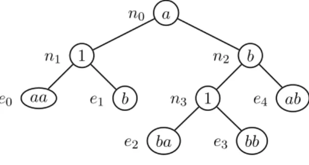
Example 4.1. For instance, the tree
(((aa, e0), (1, n1), (b, e1)), (a, n0), (((ba, e2), (1, n3), (bb, e3)), (b, n2), (ab, e4)))
is represented below n0 a n1 1 e0 aa e1 b n2 b n3 1 e2 ba e3 bb e4 ab
Figure 4.1. A factorization tree
This tree represents the iterated factorization ((aa, 1, b), a, ((ba, 1, bb), b, ab))
The yield of a tree t is the word µ(t) spelled during an inorder walk of t. It can be formally defined by structural induction as follows:
(1) if t = (u, e) then µ(t) = u,
(2) if t = (t0, (a, n), t1), then µ(t) = µ(t0)aµ(t1).
For instance, if t is the tree represented in Figure 4.1, an inorder walk of t prints, in this order, the words aa, 1, b, a, ba, 1, bb, b, ab. Therefore, the yield of this tree is aabababbbab.
The value of a tree t is the value of its yield in M , denoted by ν(t). In other words, ν = π ◦ µ. We remind the reader that the leaves of our trees are elements of R × E(M ). It follows in particular that if t has a single node, then ν(t) is necessarily an idempotent of M .
If the yield of a tree is u, the tree is called a factorization tree of u. The set F (u) of all the factorization trees of u is called the factorization forest of u. The next proposition shows in particular that F (u) is never empty. Proposition 4.1. Each word u admits a factorization tree of label π(u). Proof. If u ∈ R, then (u, π(u)) is by definition a factorization tree of u. This covers in particular the case u = 1. If u /∈ R, then by Proposition 2.2, u admits a good factorization (u0, a, u1), with a ∈ B ∪ {1}. Arguing
factorization trees t0 and t1, of label π(u0) and π(u1), respectively. We claim
that t = (t0, (a, π(u)), t1) is a factorization tree of u. First the yield of t is u.
Next, since (u0, a, u1) is a good factorization of u, π(u) <J π(u0) = λ(t0),
π(u) <J π(u1) = λ(t1) and π(u) ≤J π(a), proving the claim.
Example 4.2. Let A = {a, b, c} and let M be the syntactic monoid of the language a∗bc. Thus M is the monoid with zero presented by ({a, b, c} | a2 =
a, ab = b, ac = ba = bb = ca = cb = cc = 0). Thus M = {1, a, b, c, bc, 0}. The J -class structure of M is represented in Figure 4.2
∗0
bc b
∗a c
∗1
Figure 4.2. The J -class structure of M Some factorization trees are listed below.
in F (1): 1 1 , a 1 , 0 1 , b 1 1 1 1 1 , b 1 1 1 a 1 , b 1 a 1 1 1 , b 1 a 1 a 1 , bc 1 1 1 1 1 , bc 1 1 1 a 1 , bc 1 a 1 1 1 , bc 1 a 1 a 1 , bc 1 b 1 1 1 1 1 b 1 1 1 1 1 in F (a): a a , 0 a , etc.
in F (b): b b 1 1 1 1 , bc b 1 1 1 1 , etc. in F (c): c c 1 1 1 1 , bc c 1 1 1 1 , bc c a 1 1 1 , bc c 1 1 a 1 , bc c a 1 a 1 in F (aa): a aa , 0 aa , b 1 a a a a , bc 1 a a a a in F (ab): b b a a 1 1 , bc b a a 1 1 , b b a a a 1 , etc. in F (ac): 0 ac , bc 1 a a c c 1 1 1 1 , bc c b 1 a a 1 1 1 1 , etc. in F (abc): bc b a a c c 1 1 1 1 , bc c b b a a 1 1 1 1 , etc.
Under certain conditions, replacing a factorization tree in a factorization tree gives a factorization tree.
Proposition 4.2. Let s and s0 be two factorization trees and let p be a position in s such that λ(s|p) ≤J λ(s0). Then s[s0]|p is a factorization tree.
Proof. The result is quite intuitive, but we give nevertheless a formal proof by structural induction on s. If p is the empty word, then s[s0]
result is trivial. Assume that p = 0q for some q ∈ {0, 1}∗ (the case p = 1q would be similar). Then, if s = (s0, (a, n), s1), s[s0]|p = (s0[s0]|q, (a, n), s1).
Now, s1 is a factorization tree by definition and since λ(s0|q) = λ(s|p) ≤
λ(s0), s0[s0]|q is a factorization tree by the induction hypothesis.
Further-more, since s is a factorization tree, n ≤J π(a), n <J λ(s0) and n <J λ(s1).
Therefore, it suffices to verify that
n <J λ(s0[s0]|q) (1)
If q is the empty word, s0[s0]|q = s0 and s|p= s0. Therefore,
n <J λ(s0) = λ(s|p) ≤J λ(s0) = λ(s0[s0]|q)
which proves (1). If q is not empty, then λ(s0[s0]|q) = λ(s0), which again
gives (1).
5.
A preorder on factorization trees
We define a relation ≤ on factorization trees by structural induction: (1) If s has a single node, then s ≤ t if and only if ν(s) ≤J ν(t) and
λ(s) ≤J λ(t),
(2) If s = (s0, (a, n), s1), then s ≤ t if and only if t = (t0, (b, n), t1) with
s0 ≤ t0, s1 ≤ t1 and b ∈ {1, a}.
Some of the properties of this relation are summarized in the next proposi-tion.
Proposition 5.1.
(1) If s ≤ t, then λ(s) ≤J λ(t).
(2) If e ≤J ν(s) for some idempotent e and if s ≤ t, then e ≤J ν(t).
(3) The relation ≤ is a preorder on factorization trees.
Proof. (1) If s has a single node, then λ(s) ≤J λ(t) by definition. If
s = (s0, (a, n), s1), then λ(s) = λ(t) = n.
(2) By structural induction on s. If s has a single node, then ν(s) ≤J
ν(t) and thus e ≤J ν(s) ≤J ν(t). Otherwise s = (s0, (a, n), s1) and since
e ≤J ν(s) = ν(s0)π(a)ν(s1), e ≤J ν(s0), e ≤J π(a) and e ≤J ν(s1). Now,
since s ≤ t, t = (t0, (b, n), t1) with b ∈ {1, a}, s0 ≤ t0 and s1 ≤ t1. Then
e ≤J π(a) ≤J π(b) since b ∈ {1, a}. Applying the induction hypothesis to
s0 and s1, we get e ≤J ν(t0) and e ≤J ν(t1) and by Proposition 2.1 (4),
(3) The relation is clearly reflexive. Suppose that r ≤ s and s ≤ t. We prove that r ≤ t by structural induction on r. First, λ(r) ≤J λ(s) ≤J λ(t)
by (1). If r has a single node, then ν(r) ≤J ν(s). Since ν(r) is idempotent,
we have by (2), ν(r) ≤J ν(t), whence r ≤ t. If r = (r0, (a, n), r1), then
s = (s0, (b, n), s1), with r0 ≤ s0, r1 ≤ s1and b ∈ {1, a} and t = (t0, (c, n), t1),
with s0 ≤ t0, s1 ≤ t1 and c ∈ {1, b}. Then c ∈ {1, a} since b ∈ {1, a}, and
by induction r0≤ t0 and r1 ≤ t1. Therefore r ≤ t.
Corollary 5.2. Let s and t be trees such that s ≤ t. (1) If ν(s) is idempotent, then ν(s) ≤J ν(t).
(2) If the yield of the root of s is 1, then the yield of the root of t is also 1.
Proof. (1) is a direct consequence of Proposition 5.1 (2).
(2) By structural induction on s. Suppose first that s has a single node. Then the yield of s is the empty word, whence ν(s) = 1, and by (1), 1 ≤J
ν(t). Since M is J -trivial, it follows that ν(t) = 1, and thus the yield of t is the empty word, since we assume that π(a) 6= 1 for every a ∈ A.
If s has more than one node, then necessarily s = (s0, (1, n), s1), and
since s ≤ t, t = (t0, (1, n), t1) with s0 ≤ t0 and s1 ≤ t1. Therefore, the yield
of the root of t is 1.
However, Property 5.2 (1) fails if ν(s) is not idempotent, as shown in the next example.
Example 5.1. We take the same morphism π as in Example 4.2. Let
s = bc b a a c c 1 1 1 1 and t = bc 1 a a c c 1 1 1 1 Then s ≤ t but ν(s) = bc 6≤J ν(t) = 0.
We come back to a more positive result with the next theorem. Denote by ∼ the equivalence associated with ≤, defined by s ∼ t if and only if s ≤ t and t ≤ s.
Proof. By structural induction on s. First assume that s has a single node. Then, since t ≤ s, t also has a single node. Furthermore ν(s) ≤J ν(t) and
ν(t) ≤J ν(s), whence ν(s) = ν(t). Suppose now that s = (s0, (a, n), s1)
for some a ∈ B ∪ {1}. As s ≤ t, t = (t0, (b, n), t1), with s0 ≤ t0, s1 ≤ t1,
b ∈ {a, 1}, and as t ≤ s, t0 ≤ s0, t1≤ s1 and a ∈ {b, 1}. It follows that a = b,
s0 ∼ t0 and s1 ∼ t1, and, by induction, ν(s0) = ν(t0) and ν(s1) = ν(t1).
Therefore ν(s) = ν(s0)π(a)ν(s1) = ν(t0)π(b)ν(t1) = ν(t).
The next proposition shows that the preorder is inherited by subtrees. Proposition 5.4. Let s and t be trees such that s ≤ t.
(1) If p is a position in s, then p is also a position in t and s|p ≤ t|p. In
particular, λ(s|p) ≤J λ(t|p).
(2) If p is an internal position in s, then p is also an internal position in t. Furthermore, if the node in position p in s is (a, n), then the node in position p in t is equal to (b, n), for some b ∈ {a, 1}.
Proof. The result is clear if p is the empty word, since then, s|p = s and t|p= t. This covers the case where s has a single node. Arguing by induction on the structural complexity of s, assume that s = (s0, (a, n), s1). Then since
s ≤ t, t = (t0, (b, n), t1) with s0 ≤ t0, s1 ≤ t1 and b ∈ {a, 1}. If p = 0q for
some q ∈ {0, 1}∗, then s
|p = s0|q, t|p = t0|q, and by induction s0|q ≤ t0|q.
Therefore s|p≤ t|p.
Furthermore, if p is an internal node of s, then q is an internal node of s0. By induction, q is an internal node of t0 and hence p is an internal node
of t. Finally, if the node in position p in s is (a, n), the node in position q in s0 is also (a, n), and by induction, the node in position q in t0 is equal to
(b, n), for some b ∈ {a, 1}. But this node is also the node in position q of t. The case p = 1q is handled similarly.
We conclude this section by a result which states that, under certain conditions, the preorder ≤ is stable under replacement.
Proposition 5.5. Let s and t be trees such that s ≤ t and let p be a position in s. Then if s0 and t0 are factorization trees such that s0 ≤ t0, λ(s|p) ≤J
λ(s0) and λ(t|p) ≤J λ(t0), then s[s0]|p and t[t0]|p are factorization trees and
s[s0]
|p ≤ t[t0]|p.
Proof. The fact that s[s0]|pand t[t0]|pare factorization trees is a consequence
of Proposition 4.2.
If p is the empty word, the relation s[s0]
|p ≤ t[t0]|p reduces to s0 ≤ t0.
the structural complexity of s, assume that s = (s0, (a, n), s1). Then since
s ≤ t, t = (t0, (b, n), t1) with s0 ≤ t0, s1 ≤ t1 and b ∈ {a, 1}. Suppose that
p = 0q for some q ∈ {0, 1}∗ (the case p = 1q would be similar). Then s[s0]|p= (s0[s0]|q, (a, n), s1), t[t0]|p= (t0[t0]|q, (b, n), t1)
and by induction, s0[s0]|q ≤ t0[t0]|q. It follows that s[s0]|p ≤ t[t0]|p.
It is convenient to state separately a consequence of Proposition 5.5 which will be used in the proof of Theorem 6.4. Let (a, n) be an internal node in position p of a tree s. For each b ∈ B ∪ {1} such that n ≤J π(b), we
shall denote by s[a → b]|pthe tree obtained by replacing this node by (b, n). Corollary 5.6. Let s and t be trees such that s ≤ t and assume that s and t have the same internal node (a, n) in position p. Then, for each b ∈ B ∪ {1}, s[a → b]|p≤ t[a → b]|p.
Proof. By Proposition 5.4 (1), s|p ≤ t|p. Since p is an internal position, s|p = (s0, (a, n), s1) and thus t|p = (t0, (a, n), t1) with s0 ≤ t0 and s1 ≤ t1.
Let s0 = (s0, (b, n), s1) and t0 = (t0, (b, n), t1). By construction, s0 ≤ t0.
Furthermore, λ(s|p) = nλ(s0) and, similarly, λ(t
|p) = λ(t0). The corollary
now follows from Proposition 5.5.
6.
A preorder on words
We define a preorder on A∗ by setting u ≤ v if and only if, for each tree s ∈ F (u), there exists a tree t ∈ F (v) such that s ≤ t.
Proposition 6.1.
(1) If e ≤J π(u) for some idempotent e and if u ≤ v, then e ≤J π(v).
(2) The relation ≤ is a preorder on A∗. (3) The relation u ≤ 1 holds for every u ∈ A∗.
Proof. The first two properties follow directly from Proposition 5.1. For the last property, it suffices to verify that, for each tree s, there exists a tree t ∈ F (1) such that s ≤ t and λ(s) = λ(t). If s has a single node, say s = (u, e), one can take t = (1, e). If s = (s0, (a, n), s1), we may assume
by induction that there exist two trees t0, t1 ∈ F (1) such that s0 ≤ t0,
factorization tree, since n <J λ(s0) = λ(t0), n <J λ(s1) = λ(t1) and
n ≤J π(1). Furthermore ν(t) = ν(t0)π(1)ν(t1) = 1 and thus t ∈ F (1).
Finally s ≤ t and λ(s) = λ(t) by construction, and this completes the induction step.
Theorem 5.3 also has its counterpart on words. As for trees, we denote by ∼ the equivalence associated with the preorder ≤, defined on A∗.
The next theorem requires an auxiliary definition. Let t be a factoriza-tion tree. If we replace each leaf (u, e) of t by (π(u), e), we obtain a new tree with variables in E(M ) × E(M ), called “t modulo π”.
Theorem 6.2. The relation ∼ has finite index.
Proof. We first observe that two factorization trees with the same internal nodes and the same leaves modulo π are equivalent. It follows that if two words have the same factorization forests modulo π, they are equivalent. Now each factorization tree modulo π is a binary tree satisfying the following conditions:
(1) its depth is bounded by the J -depth of M , (2) its internal nodes are in (B ∪ {1}) × Null(M ), (3) its leaves are in E(M ) × E(M )
Since there are finitely many such trees, ∼ has finite index. Theorem 6.3. If u ∼ v, then π(u) = π(v).
Proof. Let s be a maximal element of F (u). Since u ≤ v, there exists t ∈ F (v) such that s ≤ t, and since v ≤ u, there exists s0 ∈ F (u) such that t ≤ s0. Thus s ≤ t ≤ s0 and since s is maximal, it follows s ∼ s0, whence s ∼ t ∼ s0. Therefore π(u) = ν(s) = ν(t) = π(v) by Theorem 5.3.
We are now ready to prove the main property of the preorder. Theorem 6.4. The preorder ≤ is stable on A∗.
Proof. Let u, v ∈ A∗ with u ≤ v, and let a ∈ A. By symmetry, it suffices to show that ua ≤ va. Let s ∈ F (ua). Let p be the right most position such that the yield of the node N in position p in s is not the empty word. In particular, the yield of every node on the right of N is 1.
If N is an internal node, it is of the form (a, n) for some n ∈ Null(M ), and necessarily, a ∈ B. Then s0 = s[a → 1]|pis a factorization tree for u, and
since u ≤ v, there exists a tree t0 ∈ F (v) such that s0 ≤ t0. By construction, the yield of the root of s0
|p is 1 and by Corollary 5.2 (2), the yield of the root
of t0|p is also 1. Setting t = t0[1 → a]|p and observing that s = s0[1 → a]|p, we have s ≤ t by Corollary 5.6. Furthermore, if q is a position at the right of p in s, and hence in s0, the yield of the corresponding node is 1. By Proposition 5.4, s0|q ≤ t0|q and by Corollary 5.2 (2), the yield of the node in position q in t0, and hence in t, is also 1. It follows that the yield of t is va, and hence t ∈ F (va).
Assume now that N is a leaf. By the choice of p, the yield of N is a suffix of ua and thus N = (u1a, e) for some suffix u1 of u. By Proposition
4.1, u1 has a factorization tree s1 of label π(u1). Since (u1a, e) is a leaf,
π(u1a) and e are idempotent and
e ≤J π(u1a) ≤J π(u1) = λ(s1) = ν(s1)
It follows that λ(s|p) = e ≤J λ(s1) and, by Proposition 4.2, the tree s0 =
s[s1]|p is a factorization tree of u. Note that, if q is a position of s to the
right of p, or equivalently, if q is a position of s0 to the right of s
1, then
s0|q = s|q. It follows that the yield of the node in position q in s0 is 1.
u1a s p e s1 s0 p π(u1)
Now since u ≤ v, there exists a tree t0 ∈ F (v) such that s0 ≤ t0. Let t1 = t0|p. Observing that s1 = s0|p, we have s1 ≤ t1 by Proposition 5.4. Let
q be a position of s0 to the right of s1. We have seen that the yield of the
corresponding node is 1. By Proposition 5.4, s0
|q ≤ t0|q and by Corollary 5.2
(2), the yield of the node in position q in t0 is also 1. It follows that the yield v1 of t1 is a suffix of v.
Since π(u1a) ≤J ν(s1) and s1≤ t1, Proposition 5.1 shows that
e ≤J π(u1a) ≤J ν(t1) = π(v1)
Furthermore e ≤J π(u1a) ≤J π(a) and by Proposition 2.1
e ≤J π(u1a) ≤J π(v1)π(a) = π(v1a) (2)
By Proposition 4.1, v1a has a factorization tree r of label π(v1a). Now
λ(s|p) = e ≤J π(v1a) = λ(r) and by Proposition 4.2, the tree t = s[r]|p is a
factorization tree of va.
t1 t0 p π(v1) r t p π(v1a)
We claim that (u1a, e) ≤ r. Indeed, by (2)
and
λ(u1a, e) = e ≤J π(v1a) = λ(r)
proving the claim. Thus by Proposition 5.5, s = s[(u1a, e)]|p ≤ s[r]|p =
t.
7.
Conclusion
We are now ready to prove Theorem 1.1.
Proof. Theorem 6.2 shows that the monoid N = A∗/∼ is finite.
Further-more, the preorder ≤ defined on A∗ induces a partial order, also denoted by ≤, on N . This order can be formally defined by x ≤ y if u ≤ v for some u ∈ π−1(x) and v ∈ π−1(y). Now, by Proposition 6.1 and Theorem 6.4,
(N, ≤) is an ordered monoid satisfying the identity x ≤ 1. Furthermore, Theorem 6.3 shows that M is a quotient of N .
References
[1] J. Almeida, Implicit operations on finite J -trivial semigroups and a conjecture of I. Simon, J. Pure Appl. Algebra 69, (1990), 205–218. [2] J. Almeida, Finite semigroups and universal algebra, Series in Algebra
Vol 3, World Scientific, Singapore, 1994.
[3] C. J. Ash, Finite semigroups with commuting idempotents, in J. Aus-tral. Math. Soc. Ser. A 43, (1987), 81–90.
[4] C. J. Ash, Inevitable sequences and a proof of the type II conjecture, in Proceedings of the Monash Conference on Semigroup Theory, World Scientific, Singapore, (1991), 31–42.
[5] C. J. Ash, Inevitable Graphs: A proof of the type II conjecture and some related decision procedures, Int. Jour. Alg. and Comp. 1, (1991), 127–146.
[6] K. Henckell, Blockgroups = Power Groups, in Proceedings of the Monash Conference on Semigroup Theory, World Scientific, Singapore, (1991) 117–134.
[7] K. Henckell, S. W. Margolis, J.-E. Pin and J. Rhodes, Ash’s Type II Theorem, Profinite Topology and Malcev Products, Int. Jour. Alg. and Comp. 1, (1991), 411–436.
[8] K. Henckell and J. Rhodes, The theorem of Knast, the P G = BG and Type II Conjectures, in Monoids and Semigroups with Applications, J. Rhodes (ed.), Word Scientific, (1991), 453–463.
[9] R. Knast, A semigroup characterization of dot-depth one languages, RAIRO Inform. Th´eor. 17, (1983), 321–330.
[10] R. Knast, Some theorems on graph congruences, RAIRO Inform. Th´eor. 17, (1983), 331–342.
[11] J.-E. Pin, A variety theorem without complementation, Izvestiya VUZ Matematika 39 (1995) 80–90. English version, Russian Mathem. (Iz. VUZ) 39 (1995) 74–83.
[12] J.-E. Pin, BG = PG, a success story, in NATO Advanced Study In-stitute Semigroups, Formal Languages and Groups, J. Fountain (ed.), Kluwer academic publishers, (1995), 33–47.
[13] J.-E. Pin and P. Weil, Polynomial closure and unambiguous product, Theory Comput. Systems 30, (1997), 1–39.
[14] J.-E. Pin and P. Weil, Semidirect product of ordered monoids, in prepa-ration.
[15] J.-E. Pin and P. Weil, The wreath product principle for ordered semi-groups, in preparation.
[16] I. Simon, Piecewise testable events, Proc. 2nd GI Conf., Lect. Notes in Comp. Sci. 33, Springer Verlag, Berlin, Heidelberg, New York, (1975), 214–222.
[17] I. Simon, Properties of factorization forests, in Formal properties of finite automata and applications, J.-E. Pin (ed.), Lect. Notes in Comp. Sci. 386, Springer Verlag, Berlin, Heidelberg, New York, (1989), 34–55. [18] I. Simon, Factorization forests of finite height, Theor. Comp. Sc. 72,
(1990), 65–94.
[19] I. Simon, A short proof of the factorization forest theorem, in Tree Au-tomata and Languages, M. Nivat and A. Podelski eds., Elsevier Science Publ., Amsterdam, (1992) 433–438.
[20] H. Straubing and D. Th´erien, Partially ordered finite monoids and a theorem of I. Simon, J. of Algebra 119, (1985), 393–399.