Tropospheric ozone budget: regional and global calculations

(1)

HAL Id: hal-00301118

https://hal.archives-ouvertes.fr/hal-00301118

Submitted on 11 Feb 2004

HAL is a multi-disciplinary open access

archive for the deposit and dissemination of sci-entific research documents, whether they are pub-lished or not. The documents may come from teaching and research institutions in France or abroad, or from public or private research centers.

L’archive ouverte pluridisciplinaire HAL, est destinée au dépôt et à la diffusion de documents scientifiques de niveau recherche, publiés ou non, émanant des établissements d’enseignement et de recherche français ou étrangers, des laboratoires publics ou privés.

Tropospheric ozone budget: regional and global

calculations

F. M. O’Connor, Kathy S. Law, J. A. Pyle, H. Barjat, N. Brough, K. Dewey,

T. Green, J. Kent, G. Phillips

To cite this version:

F. M. O’Connor, Kathy S. Law, J. A. Pyle, H. Barjat, N. Brough, et al.. Tropospheric ozone bud-get: regional and global calculations. Atmospheric Chemistry and Physics Discussions, European Geosciences Union, 2004, 4 (1), pp.991-1036. �hal-00301118�

(2)

ACPD

4, 991–1036, 2004

Regional and global ozone budget F. M. O’Connor et al. Title Page Abstract Introduction Conclusions References Tables Figures J I J I Back Close Full Screen / Esc

Print Version Interactive Discussion

www.atmos-chem-phys.org/acpd/4/991/ SRef-ID: 1680-7375/acpd/2004-4-991 © European Geosciences Union 2004

Atmospheric Chemistry and Physics Discussions

Tropospheric ozone budget: regional and

global calculations

F. M. O’Connor1, K. S. Law2, a, J. A. Pyle1, H. Barjat3, b, N. Brough4, K. Dewey3, T. Green4, J. Kent3, and G. Phillips5, c

1

NCAS-Atmospheric Chemistry Modelling Support Unit, Centre for Atmospheric Science, University of Cambridge, United Kingdom

2

Centre for Atmospheric Science, University of Cambridge, United Kingdom 3

Met. Research Flight, United Kingdom 4

School of Environmental Sciences, University of East Anglia, United Kingdom 5

Department of Chemistry, University of Leicester, United Kingdom a

Now at Service d’A ´eronomie/IPSL, Paris, France b

Now at Centre for Atmospheric Science, University of Cambridge, United Kingdom c

Now at Geophysical Institute, University of Alaska Fairbanks, USA

Received: 6 January 2004 – Accepted: 2 February 2004 – Published: 11 February 2004 Correspondence to: F. M. O’Connor (fiona.oconnor@atm.ch.cam.ac.uk)

(3)

ACPD

4, 991–1036, 2004

Results from a tropospheric three-dimensional chemical transport model (TOMCAT) have been used to examine the terms of the ozone budget, both regionally and glob-ally. The global calculations are discussed in light of other published estimates. Re-gional budgets are calculated for continental regions, including the American Mid-West,

5

Sahara, and central Europe. These are compared with regional budgets for oceanic regions, including the Azores High and the Tropical Pacific Warm Pool. Furthermore, the coastal region of the UK and Ireland is also considered. The validity of these regional budgets from TOMCAT are discussed by comparing TOMCAT with measure-ments from a number of aircraft campaigns. The budgets for central Europe and the

10

American Mid-West indicate that continental regions dominate the ozone budget of the northern extratropics. This is in spite of the remote oceanic regions being photochemi-cal sinks for ozone. The regional budget photochemi-calculations for the UK and Ireland exhibit net photochemical production of ozone in the boundary layer but this is not consistent with available aircraft measurements. This is attributed to the coarse horizontal resolution

15

of the TOMCAT model which results in the model’s photochemical budget being more typical of a polluted continental region than a relatively remote one. On the other hand, the ozone photochemical rates calculated for the Azores High and the Tropical Pacific Warm Pool agree rather well with other estimates.

1. Introduction

20

Although only a trace gas, ozone plays an important role in the atmosphere both radia-tively and chemically. Stratospheric ozone, for example, prevents shortwave ultraviolet (UV) radiation reaching the Earth’s surface. As a result, stratospheric ozone deple-tion can cause increased UV levels at the Earth’s surface, with implicadeple-tions for human health (e.g. DeGruijl et al., 2003), animal and plant life (e.g. Caldwell et al., 2003).

25

(4)

ACPD

4, 991–1036, 2004

least as important a greenhouse gas as methane (Mickley et al., 2001). In the tropo-sphere, ozone is also the precursor for the main tropospheric oxidising agents, the hy-droxyl (OH) and nitrate (NO₃) radicals. Consequently, tropospheric ozone has a strong influence on the ability of the troposphere to remove greenhouse gases and other

pol-5

lutants such as non-methane hydrocarbons (NMHCs). However, surface ozone is a pollutant and is detrimental to people with respiratory problems (e.g. Peden, 2001) and ecosystems (e.g. Nali et al., 2002). High levels of ozone at the surface are already an air quality problem in much of the Northern Hemisphere and predictions reported by Prather et al. (2003) show that air quality standards, in relation to ozone, may be further

10

violated in the coming decades if the model calculations and the proposed emission scenario are correct. However, there is still a large degree of uncertainty in the factors which control ozone in the troposphere (Prather et al., 2001). As a result, there is a need for better quantitative understanding of these factors, such that more accurate projections for the future can be made.

15

For a long time, it was believed that tropospheric ozone was controlled by a bal-ance between stratosphere-troposphere exchange (STE) processes (Holton et al., 1995) and loss at the surface through dry deposition. In the early 1970s, however, Crutzen (1973) and Chameides and Walker (1973) suggested that photochemical oxi-dation of carbon monoxide (CO) and hydrocarbons, catalysed by NO_x and HO_x, could

20

be a significant tropospheric source of ozone. Numerous studies have since been carried out on in-situ ozone photochemistry in different regions. It was found that pho-tochemistry can result in either a net photochemical loss or gain of ozone depending on the environment. Over continental areas, significant net ozone production can occur in the boundary layer close to source regions (e.g. Frost et al., 1998). On the other hand,

25

the net effect of photochemistry in the boundary layer of remote regions is generally to destroy ozone (e.g. Carpenter et al., 1997; Monks et al., 2000). However, mea-surements downwind of continental regions suggest that continental outflow of ozone precursors can result in net ozone production over remote regions, even at the

(5)

low-ACPD

4, 991–1036, 2004

ozone production can also occur in the free troposphere over continental regions (e.g. Zanis et al., 2000) due to transport of ozone precursors from the polluted boundary layer into the free troposphere as a result of frontal activity (e.g. Bethan et al., 1998) and/or convection (Dickerson et al., 1987) or from in-situ sources, such as lightning

5

and aircraft emissions. Although there is net destruction of ozone at lower levels over remote regions, it is often accompanied by small but positive net ozone production rates aloft (e.g. Davis et al., 1996; Reeves et al., 2002); this can be attributed to long-range transport, the increased lifetime of NO_x (Liu et al., 1987) and the relatively low concentrations required to maintain net ozone production in the upper troposphere.

10

Given that the lifetime of ozone in the troposphere is quite long, the distribution of tro-pospheric ozone is also influenced by transport across the tropopause. Although cross-tropopause transport can occur in both directions, the net global effect of stratosphere-troposphere exchange (STE) events, in terms of ozone, is downward transport of ozone-rich air from the stratosphere into the troposphere. Numerous studies have

15

been published on observations of stratospheric air in the troposphere associated with synoptic-scale and mesoscale processes, such as convective events (Poulida et al., 1996) and in particular, tropopause folds near jetstreams (e.g. Vaughan et al., 2001) and cut-off lows (Price and Vaughan, 1993). Ozone-rich air from the stratosphere can penetrate quite deeply into the troposphere and has even been associated with

20

episodes of high ozone concentrations at the surface (Davies and Schuepbach 1994). Furthermore, layers of stratospheric air can be quite persistent (Bithell et al., 2000), given the lifetime of ozone in the troposphere (Liu et al., 1987). Stratospheric air transported into the troposphere can, therefore, contribute directly and significantly to the tropospheric ozone budget (Fabian and Pruchniewicz, 1977) and affect surface

25

air quality standards in relation to ozone. Due to the different chemical characteristics of stratospheric and tropospheric air, Pierrehumbert and Yang (1993) noted that air masses of different composition will be brought close together following STE events. Indeed, Methven et al. (2003) recently reported on aircraft observations of a

(6)

strato-ACPD

4, 991–1036, 2004

pol-luted boundary layer air. Over time, these layers of differing chemical characteristics will be stretched to smaller and smaller scales giving rise to efficient mixing between the air masses. Parrish et al. (2000), for example, presented a case study from the North At-lantic winter troposphere, in which air of anthropogenic origin mixed with stratospheric

5

air. The effect of mixing high-ozone air with tropospheric water vapour was proposed to lead to enhanced production of hydroxyl radicals by Esler et al. (2001), thereby in-fluencing the tropospheric oxidising capacity.

In addition to photochemistry and STE, the third term which has a direct impact on the tropospheric ozone burden and budget is dry deposition. This is a process by which

10

certain trace species are transferred from the atmosphere to the Earth’s surface and then lost at the surface by chemical, physical, and biological processes in the absence of precipitation. Dry deposition fluxes of trace species are parameterised in models as the trace gas concentration multiplied by a deposition velocity. Deposition velocities, themselves, are extremely difficult to measure, although it is evident that they depend

15

strongly on surface characteristics (e.g. Fuentes et al., 1992; Lenschow et al., 1982). Natural surfaces, such as plant leaves, act as relatively efficient sinks but deposition velocities are also affected by diurnal and seasonal cycles in plant activity. On the other hand, water does not provide an efficient surface for dry deposition. In the case of ozone, estimates of the ratio between the hemispheres for this loss range between

20

1.5 and 3 (Galbally and Roy, 1980). This difference between the hemispheres reflects that deposition rates are much more efficient over land than ocean.

Given that the net effect of photochemistry is region-dependent and that tropospheric ozone is influenced by long-range transport of pollutants as well as cross-tropopause transport, three-dimensional chemical modelling is required to quantify the various

25

terms of the global ozone budget. The purpose of the current study is to examine global and regional ozone budgets using the global TOMCAT model. The model is first described in Sect.2and a summary of model intercomparison and validation studies is given in Sect.3. Seasonal and annual global budget calculations will be presented in

(7)

ACPD

4, 991–1036, 2004

In Sect.5, regional budget calculations are discussed and validated in certain cases using available aircraft observations and/or other estimates. Some concluding remarks will be presented in Sect.6.

2. The TOMCAT model

5

The model used in this study is the three-dimensional chemical transport model (CTM), TOMCAT (Law et al., 1998; Law et al., 2000). Advection is performed using the second order moment scheme of Prather (1986) and forced with meteorological analyses from the European Centre for Medium-Range Weather Forecasts (ECMWF). The resolution of TOMCAT is approximately 2.8◦by 2.8◦ in the horizontal. There are 31 levels

extend-10

ing up to 10 hPa in the vertical, which are defined as terrain-following sigma levels near the surface, pure pressure levels in the stratosphere and a hybrid of the two types in the intermediate levels; the resolution is approximately 40 hPa in the mid and upper troposphere.

The moist convection parameterisation implemented in TOMCAT is the mass flux

15

scheme of Tiedtke (1989). It includes convective updrafts and large-scale subsidence associated with deep and shallow convection, as well as turbulent and organised en-trainment and deen-trainment. Coupled to the convection scheme, both in time and space, are lightning emissions of NO_x, which were implemented by Stockwell et al. (1999). The only difference here is that the lightning emissions were scaled to give a global

an-20

nual total of 5 Tg N year−1in line with Prather et al. (2001) from the Third Assessment Report (TAR) of the Intergovernmental Panel on Climate Change (IPCC).

TOMCAT uses the Holtslag and Boville (1993) non-local vertical diffusion scheme from the National Center for Atmospheric Research (NCAR) Community Climate Model, Version 2 (CCM2). This scheme determines the planetary boundary layer (PBL)

25

height explicitly and takes account of large eddy transports that can occur throughout the boundary layer even when part of it is statically stable. Implementation and

(8)

valida-ACPD

4, 991–1036, 2004

The chemical scheme in TOMCAT considers 48 species that describe CH₄ -CO-NMHC-NO_xchemistry, of which 27 are advected. The model accounts for 28 photodis-sociation, 89 bimolecular, and 15 termolecular reactions; no heterogeneous chemistry is included. The chemical species are treated as chemical families with the ASAD code

5

(Carver et al., 1997) which uses the IMPACT time integration scheme of Carver and Stott (2000). Bimolecular and termolecular rate coefficients are taken from DeMore et al. (1997) and Atkinson et al. (1997). Photolysis rates are calculated off-line in the Cambridge 2D model (Law and Pyle, 1993) with the Hough (1988) scheme. This takes account of multiple scattering by clouds using a climatological cloud cover dataset and

10

a fixed aerosol profile. The Cambridge 2D model (Law and Pyle, 1993) is also used to provide boundary conditions for ozone, NO_y and CH₄ at the top of TOMCAT, which is currently at 10 hPa.

Emissions of NO_x, CO, CH₄ and NMHCs are included in TOMCAT. NO_x emissions are added according to the recommendations used in the TAR of the IPCC (Prather

15

et al., 2001) and include industrial, biomass burning, soil, aircraft, and lightning emis-sions. A seasonal variation is applied to the biomass burning emissions according to Hao and Liu (1994). The global annual total of NO_x emissions is 44.4 Tg N year−1. Emissions of CO from industry, biomass burning, vegetation, and oceans are also according to the IPCC TAR (Prather et al., 2001), with the same seasonality

ap-20

plied to the CO biomass burning emissions as for NO_x. An additional 220 Tg CO is also emitted to take account of isoprene oxidation, giving a global annual emission of 1770 Tg CO year−1.

Methane emissions in TOMCAT include emissions from termites (Sanderson, 1996), animals, biomass burning and gas (M ¨uller and Brasseur 1995), mining (M ¨uller, 1992),

25

landfills and sewage (M ¨uller and Brasseur, 1995), rice paddies (Aselmann and Crutzen, 1989), wetlands, and the ocean. A soil sink is also taken into account (Dorr et al., 1993), giving a net annual emission of 517 Tg CH₄ year−1. Emissions of ethane (16 Tg year−1), propane (16 Tg year−1) and aldehydes are included. For

(9)

formalde-ACPD

4, 991–1036, 2004

from biomass burning after Yokelson et al. (1997) and an additional 1 Tg from indus-tral sources (Shallcross, 1999). For methylaldehyde (MeCHO), 0.3 Tg is emitted. Fi-nally, a global annual emission of acetone of 50 Tg is added according to the IPCC TAR (Prather et al., 2001).

5

TOMCAT also takes account of loss at the surface through the process of dry de-position, using prescribed deposition velocities at 1 metre above the ground (Valentin, 1990 and references therein) which are dependent on surface type, season, and time of day. They are then extrapolated from 1 metre to the centre of the bottom gridbox, according to Berntsen and Isaksen (1997), using the vertical diffusion coefficient

calcu-10

lated explicitly by the model’s PBL scheme. In this way, the model’s dry deposition loss rates are dependent on wind velocity, surface roughness and the stability of the bound-ary layer. The wet deposition scheme uses the model’s convective and large-scale rainfall, following a scheme originally developed by Walton et al. (1988). The scheme uses the scavenging coefficient values for nitric acid (HNO₃) proposed by Penner et

15

al. (1991), which are scaled down according to the fraction of each species in the liquid phase determined by Henry’s Law. Both the wet and dry deposition schemes have been implemented and validated in TOMCAT by Giannakopoulos et al. (1999).

3. Model validation

Various studies have been carried out to validate the TOMCAT model. Law et

20

al. (1998), for example, compared ozone data collected on passenger aircraft as part of the Measurement of Ozone by Airbus In-Service Aircraft (MOZAIC) project with mod-elled ozone from the TOMCAT model. They found that the model showed good agree-ment with seasonally averaged data at cruise altitudes in the upper troposphere/lower stratosphere (UTLS) region and with individual vertical profiles collected during takeoff

25

and landing. The TOMCAT model was further validated by participating in a com-parison of several CTMs with two years of MOZAIC data by Law et al. (2000). The

(10)

ACPD

4, 991–1036, 2004

it did show a tendency to overestimate ozone at cruise altitudes in the tropics and mid-latitudes. This was attributed by the authors to an overly strong stratospheric circulation and/or the treatment of ozone at the top boundary.

More recently, modelled ozone from the TOMCAT model was compared with a larger

5

set of three-dimensional models and evaluated using ozonesonde and ground-based observations in a study by Prather et al. (2001). Here, TOMCAT was able to reproduce the seasonal cycle of ozone at various latitudes, although it overestimated ozone in the mid and upper troposphere, particularly at northern high latitudes. This study also included a comparison of the models with observations of CO from surface sites at a

10

variety of altitudes and latitudes. TOMCAT performed very well in capturing the sea-sonal cycle in observed CO in the tropics and in the northern mid and high latitudes. However, TOMCAT, in addition to the other models, overestimated CO at the remote site of Cape Grim, suggesting that Southern Hemisphere emissions of CO were over-estimated in the IPCC recommendations.

15

In the study by Prather et al. (2001), they also noted that the available databases of NO_x measurements at that time (Emmons et al., 1997; Thakur et al., 1999) were not extensive enough to provide an adequate test of global models, due to the large spatial variability in emissions of NO_x from industrial sources, lightning, and biomass burning. The EU-funded TRADEOFF project has gone some way to address this by

20

compiling a new database of in-situ measurements from several measurement cam-paigns which were not included in Emmons et al. (2000). In particular, measurements of NO_y species and peroxides have been included. This database has very recently been used to perform a rigorous evaluation of two General Circulation Models (GCMs) and five CTMs, one of which was the TOMCAT model (Brunner et al., 2003). In

TOM-25

CAT, it was found that mixing across the tropopause was too strong, resulting in high modelled concentrations of CO in the lowermost stratosphere and high ozone concen-trations in the upper troposphere. Comparison with NO_x measurements indicated that TOMCAT underestimated NO_x over north America both in the mid troposphere and in

(11)

ACPD

4, 991–1036, 2004

good agreement with observations at northern midlatitudes. Each model in this study had particular strengths and weaknesses; generally the TOMCAT behaviour was sat-isfactory in comparison with the other models.

4. Global annual ozone budget

5

For the work here, TOMCAT was initialised on 1 January 2000 from a previous model integration and forced by ECMWF analyses. The analysis were interpolated from their original 60 levels to 31 levels, which extend from the surface up to 10 hPa. TOMCAT was integrated until May 2001, allowing 4 further months for model spin-up and a total of 12 months for the global annual budget calculations. The net photochemical term

10

of the ozone budget was calculated by integrating the difference in the tropospheric ozone burden before and after the chemistry scheme in TOMCAT through the time period of interest. A combined tropopause was used to define the troposphere – the 380 K isentropic surface in the tropics and the 3.5 PVU surface in the extratropics. The stratospheric input was calculated in the same way, although in this case, the difference

15

used was that of the ozone burden before and after the call to the transport scheme. This was considered an appropriate method to calculate STE because the model’s advective mass fluxes are highly variable and it was found that the calculation of the stratospheric flux using these fluxes was very sensitive to the sampling frequency and the time period considered. For the dry deposition loss term, the ozone burden in the

20

bottom gridbox of the model was output every chemical timestep along with the first order loss rate due to deposition. In this way, the integrated effect of dry deposition could be evaluated. Table1 shows the tropospheric source and sink terms and the tropospheric ozone burden for three regions (the northern extratropics, tropics, and the southern extratropics) and four seasons (December, January, and February; March,

25

April, and May; June, July, and August; September, October, and November). Global and annual terms are given as well as the residual, which is defined as the sum of the

(12)

ACPD

4, 991–1036, 2004

The net effect of photochemistry in TOMCAT shows a strong seasonal cycle, with maximum net ozone production during the JJA season in the northern extratropics. This can be attributed to the enhanced photochemical production occurring during summer in the Northern Hemisphere and is in qualitative agreement with other

mod-5

elling studies (Hauglustaine et al., 1998; Roelofs and Lelieveld, 1995). TOMCAT also indicates that the annual global net ozone production is equally divided between the tropics and the northern extratropics and is consistent with a study of present and pre-industrial tropospheric ozone by Levy et al. (1997). Despite the qualitative agreement between TOMCAT and other models in regard to the seasonal and regional

contribu-10

tions, the quantitative agreement is not so robust. On a global scale, the net photo-chemical term from a number of global chemistry models was reported by Prather et al. (2001) to be in the range from −850 to+500 Tg O₃ year−1. This suggests that in some models, the troposphere is a photochemical sink for ozone while others predict that the troposphere is a net source of ozone. However, in EC (2003), the range was

15

reported as+70 to +880 Tg O₃year−1. The value of+664 Tg O₃year−1from TOMCAT is at the upper end of this range although it is very similar to that reported recently by Zeng and Pyle (2003), who used the same chemistry scheme as TOMCAT in the UK Met Office’s Unified Model. The large discrepancy between models, not only in the sign of the photochemical impact but also in its magnitude, highlights the uncertainty

20

which still remains. Part of this uncertainty is due to the net photochemical term being the sum of two large but oppositely signed terms. However, the discrepancy has also been attributed to the large uncertainty in the influence of stratospheric ozone on the troposphere (Prather et al., 2001; Zeng and Pyle, 2003).

In the IPCC TAR, Prather et al. (2001) highlighted the range of estimates for the

25

contribution of stratosphere-to-troposphere transport on the tropospheric ozone bud-get from a large number of models involved in the OxCOMP intercomparison exer-cise; the range was 390–1440 Tg O₃ year−1. The value of 851 Tg O₃ year−1 for the global annual stratospheric flux calculated here is well within the range reported by

(13)

ACPD

4, 991–1036, 2004

of the stratosphere on tropospheric ozone in the present-day atmosphere. Given that stratosphere-to-troposphere exchange is sensitive to model resolution (Kentarchos et al., 2000), the range of estimates may be partly due to the range of resolutions used by the models. Results are also sensitive to the definition of the tropopause used. For

5

future predictions, however, the uncertainty may be even further complicated by the in-crease in the mass exchange between the stratosphere and troposphere expected due to a changing climate (Butchart and Scaife, 2001). Despite the uncertainty in the global annual estimates themselves, there is some consistency between models. For exam-ple, TOMCAT predicts that the global stratospheric flux shows a seasonal cycle, with

10

maximum fluxes in DJF and MAM, consistent with other modelling studies (Wauben et al., 1998; Roelofs and Lelieveld, 1995; Lelieveld and Dentener, 2000). TOMCAT, however, does not exhibit such a strong seasonal cycle as in other models, which may be the result of a poor seasonal cycle in the boundary conditions prescribed at 10 hPa or due to a lack of resolved dynamics in the stratosphere. TOMCAT also indicates that

15

significant downward transport of ozone occurs in the tropics, associated with breaks in the subtropical jetstreams and is consistent with the tropical upwelling being limited to equatorward of ±15◦ latitude except in the Southern Hemisphere winter (Rosenlof and Holton, 1993).

As well as transport and photochemistry, the third term which influences the global

20

ozone budget is dry deposition. From TOMCAT, the dry deposition term in the northern extratropics demonstrates a seasonal cycle, with maximum deposition occurring during the Northern Hemisphere summer. This is consistent with photochemical production of ozone being a maximum in JJA and the increased vertical mixing in the boundary layer during summer. A similar result has been found by Bernsten and Isaksen (1997),

25

Roelofs and Lelieveld (1997), and Hauglustaine et al. (1998). Furthermore, TOMCAT indicates that ozone is very efficiently deposited in the tropics, particularly during the Northern Hemisphere summer. This may be the result of the subsidence of relatively ozone-rich air from the upper troposphere associated with convection and/or the

(14)

occur-ACPD

4, 991–1036, 2004

Ozone in the southern extratropics, on the other hand, is not strongly deposited, partly because of low ozone concentrations but also because deposition over the ocean is not as efficient as over land. Again, a comparison of the global estimates for the loss of ozone at the surface by dry deposition was presented by Prather et al. (2001). The

5

range of estimates was 530–1200 Tg O₃year−1. This term is dependent on the depo-sition velocities used by the models, the modelled surface ozone concentrations and the efficiency of mixing within their respective boundary layers. A dry deposition term of 1529 Tg O₃ year−1 from TOMCAT is high relative to the other models, whose max-imum deposition term was approximately 1200 Tg O₃year−1. This may be indicative

10

of the modelled surface ozone concentrations being too high in TOMCAT although this is not apparent in ozonesonde comparisons (e.g. Prather et al., 2001). Alternatively, it may be suggestive of a too well-mixed boundary layer (Granier et al., 2003), in which relatively ozone-rich air is being efficiently transported down into the bottom gridbox and then deposited.

15

Finally, the mean global tropospheric ozone burden was found to be 297 Tg O₃, using the combined 380 K and 3.5 PVU surfaces to define the tropopause. This estimate is well within the range of 270–370 Tg O₃ reported by Prather et al. (2001) although TOMCAT does tend to overestimate ozone in the upper troposphere (Law et al., 2000; Brunner et al., 2003). A spring/summer ozone maximum is also evident in the northern

20

extratropics. Many observational studies indicate that the spring ozone maximum is a hemispheric phenomenon (e.g. Oltmans and Levy III 1994; Fishman and Brackett, 1997) and results from TOMCAT suggest that it is due to combined contributions from STE and photochemical production of ozone. STE peaks in DJF but is still significant in MAM, while photochemical production of ozone rapidly increases between the DJF and

25

MAM seasons. A modelling study by Wang et al. (1998) came to a similar conclusion although they found that chemistry was the most important factor. A review of the observations and origins of the spring ozone maximum can be found in Monks (2000). Given these results and the large uncertainty in the various terms of the global ozone

(15)

ACPD

4, 991–1036, 2004

sections, TOMCAT is used to evaluate the ozone budgets over various regions, some of which have been sampled by intensive aircraft measurement campaigns. In this way, the validity of the modelled regional budgets can be assessed.

5. Regional ozone budgets

5

Six regions are considered; these are indicated in Table 2 along with the size of the region and illustrated in Fig. 1. Budgets for one coastal, three continental, and two oceanic regions have been calculated and are discussed below.

5.1. UK and Ireland

The domain considered here was chosen to extend from 50◦N to 60◦N and from 10◦W

10

to 0◦W. Although the region to be considered is quite limited, it was chosen to coin-cide with the area sampled by an aircraft campaign (see below). Table3 shows the ozone budget for the region encompassing the UK and Ireland as a function of season. It indicates that the region, on an annual basis, is a photochemical source of ozone and an exporter of ozone. There is significant net ozone production in the Northern

15

Hemisphere summer (JJA) but weak net ozone destruction in DJF. The transport term, which is the net effect of STE and horizontal transport, suggests that the region is a net exporter of ozone in all seasons except SON; this is most likely due to net photo-chemical production of ozone being quite weak in SON but deposition at the surface still being relatively strong.

20

The validity of the ozone budget for the UK and Ireland region, presented in Table3, can be assessed to some extent by a comparison of TOMCAT with available mea-surements from the region. During May 2000, an aircraft campaign involving the UK Met Office C-130 aircraft took place over Scotland as part of the ACTO (Atmospheric Chemistry and Transport of Ozone) project. The aircraft was equipped to take

(16)

ACPD

4, 991–1036, 2004

Fig-ure2shows the flight tracks of the C-130 aircraft during the entire campaign. Although the aircraft principally flew over the marine sector, a large variety of air masses was sampled, including stratospheric air, polluted continental boundary layer air and clean marine boundary layer air. The last flight of the ACTO campaign has been discussed

5

in more detail by Methven et al. (2003).

Figure 3a shows modelled net ozone production rates, calculated along the flight tracks, plotted as a function of pressure. It indicates that there is net ozone pro-duction in the boundary layer over the UK and Ireland region with maximum rates of +3.5 ppbv hour−1. Carpenter et al. (1997), however, found that the NO compensation

10

point (the concentration of NO above which net ozone production occurs) in the bound-ary layer at Mace Head, Ireland during Spring was between 26 and 84 pptv NO. From Fig.3b, in which modelled and measured NO concentrations are plotted, the measured NO concentrations in the boundary layer during ACTO are of the order of 0–50 pptv, and are therefore more consistent with either weak net ozone production or destruction.

15

Modelled NO concentrations are strongly overestimated in the lowest 2 km, leading to modelled net ozone production rates in the boundary layer over the UK and Ireland re-gion which are too strongly positive. This can most likely be attributed to the proximity of the region to continental Europe and the coarse horizontal resolution of TOMCAT, resulting in the model’s boundary layer having NO concentrations more typical of a

20

continental boundary layer than a remote one. Although TOMCAT indicates that there is photochemical production of ozone in the boundary layer in this region, modelled ozone itself is not overestimated, as indicated in Fig.3c. This suggests that sufficient ozone is being lost through dry deposition to counteract the net ozone production. As a result, it is likely that dry deposition over this region has also been overestimated.

25

In the free troposphere, modelling some flights from the ACTO campaign suggests that there is net ozone destruction, albeit small (e.g. Flight A755 in Fig.3a) whereas other flights have a slightly positive net ozone production rate (e.g. Flight 754). How-ever, on average, the net ozone production rates are close to zero. This result is

(17)

ACPD

4, 991–1036, 2004

investigate the contribution of photochemistry to the winter-spring ozone maximum in the Northern Hemisphere mid-latitude free troposphere. They found that there is net photochemical production of ozone at 500 hPa between 30 and 60◦N during the winter period but that in May, the region is in photochemical balance. However, their model

5

simulation also suggested that there is net ozone production in the lower free tropo-sphere (685 hPa) of this region in May and, although this is what is also predicted by TOMCAT, it is not consistent with the ACTO measurements.

5.2. Central Europe

The seasonal and annual ozone budget for part of central Europe can be found in

10

Table 3. In this region there is always net photochemical production of ozone, with maximum net production during the Northern Hemisphere summer (JJA). This coin-cides with a maximum in loss of ozone at the surface through dry deposition. This seasonal variation in photochemistry and dry deposition over central Europe is similar to that for the whole of the northern extratropics, suggesting that the budget for the

15

northern extratropics is dominated by that of the continental regions. The transport term, including both horizontal transport into/out of the region and STE, indicates that the region exports ozone in all seasons except MAM.

TOMCAT shows that net ozone production over central Europe is a maximum in JJA and Fig.4 shows the modelled net ozone production rates, calculated along aircraft

20

flight tracks from the EXPORT (European eXport of Precursors and Ozone by long-Range Transport) campaign (see below), plotted as a function of pressure. It indicates that there is net ozone production in the boundary layer over central Europe during July/August 2000, with a range of 1.0–3.5 ppbv hour−1. An analysis of the ozone ten-dency in polluted air masses arriving at Mace Head from Britain and continental

Eu-25

rope by Salisbury et al. (2002) showed that the mean net ozone production rate during summer was 2.9 ppbv hour−1, consistent with our modelled estimates. Furthermore, constrained box model calculations based on aircraft observations from the EU-funded

(18)

ACPD

4, 991–1036, 2004

net ozone production rates of up to 4 ppbv hour−1were encountered in polluted bound-ary layer air (Hov et al., 2000). Whereas over western Europe, the free troposphere ap-peared to be strongly decoupled from the boundary layer (see Fig.3a), Fig.4suggests that there is significant transport of boundary layer air and ozone precursors into the

5

free troposphere. Indeed, rapid uplift associated with embedded convection in a warm conveyor belt resulted in elevated concentrations of NMHCs being observed in the mid troposphere (Purvis et al., 2003). This boundary layer to free troposphere transport results in net ozone production rates of the order of 0.0–1.0 ppbv hour−1 in the free troposphere. These rates are higher than ozone tendencies evaluated from free

tropo-10

spheric measurements at Jungfraujoch in the Swiss Alps for April/May 1996 by Zanis et al. (2000), who found net ozone production rates of the order of 0.1–0.3 ppbv hour−1 in background conditions. Here, however, the rates are more strongly positive, consis-tent with the uplift of recently polluted air masses from the boundary layer into the free troposphere and higher photolytic activity. A modelling study by Yienger et al. (1999)

15

suggests that the global free troposphere between 30 and 60◦N during JJA is pho-tochemically destroying ozone. However, they did find that net production still occurs over the polluted continents, as is the case here.

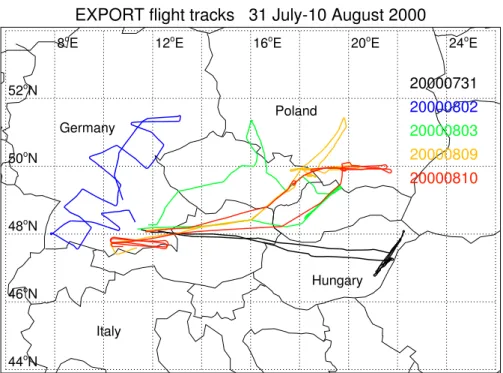
Although the modelled rates from TOMCAT for July/August 2000 appear to agree with other studies, the extent to which they are consistent with the EXPORT aircraft

20

measurements will be investigated next by examining individual production and de-struction pathways. During the EXPORT campaign in July/August 2000, the C-130 aircraft was based at Oberpfaffenhoffen, near Munich, and sampled air over central and eastern Europe between 0 and 8 km. The flight tracks are shown in Fig.5. The air sampled on the flights was quite polluted, with very recent uplifted boundary layer air

25

being sampled in the free troposphere. Some of the measurements taken during this campaign and the mechanisms for tranporting air from the boundary layer into the free troposphere have been discussed recently by Purvis et al. (2003).

(19)

re-ACPD

4, 991–1036, 2004

and water vapour concentrations along the EXPORT flight tracks and their modelled equivalents allow a direct comparison of measured and modelled in-situ ozone loss rates by this process. Figure6a shows the comparison for the EXPORT flights, with the points coloured according to altitude. Both modelled and measured in-situ ozone

5

loss rates due to the reaction of O1D and water vapour decrease with altitude. This is primarily due to the reduction of available water vapour, which is not compensated for by the higher photolysis rates and increasing ozone concentrations. This was also found by Reeves et al. (2002) who calculated ozone production and loss rates us-ing a box model constrained by sprus-ingtime aircraft measurements over the North

At-10

lantic. Here, the modelled and measured ozone loss rates compare very well when the loss rates are relatively small at higher altitudes. However, measured loss rates of greater than 0.3 ppbv hour−1 are not well captured by TOMCAT. A maximum loss rate of 0.3 ppbv hour−1 was calculated by Reeves et al. (2002) for comparable ozone and water vapour concentrations. However, the higher measured ozone loss rates here are

15

consistent with higher photolysis rates during summer. Given that the comparison be-tween modelled and measured ozone and water vapour concentrations was quite good during EXPORT (Fig.7), the discrepancy in the in-situ loss rates is attributed to di ffer-ences in modelled and measured j(O1D) rates (not shown). For TOMCAT, photolysis rates are calculated off-line in the Cambridge 2D model (Law and Pyle 1993), using a

20

two-stream approach and a climatological cloud field. This results in modelled photoly-sis rates which are generally lower than those measured on the aircraft, particularly at lower altitudes. A similar result was found for a comparison from the ACTO campaign (not shown). The modelled photolysis rates are still too low at lower altitudes even in the absence of cloud, suggesting that it could be due to the 2D model’s vertical ozone

25

distribution or ozone column or its treatment of surface albedo. However, equally, the discrepancy may be the result of uncertainties in the measurements of j(O1D). These measurements are difficult to make and have an accuracy of approximately 13 % in clear sky conditions. In cloudy conditions, the uncertainty is probably even greater.

(20)

ACPD

4, 991–1036, 2004

taken on board the C-130 aircraft according to Brough et al. (2003) and Green et al. (2003), respectively. Using these measurements, situ ozone production rates, in-volving modelled and measured concentrations of NO and CH₃O₂radicals, can also be compared. Figure6b shows a comparison of the in-situ ozone production rate along the

5

EXPORT flight tracks. Ozone production from the NO/CH₃O₂pathway decreases sub-stantially with altitude as a result of lower NO and radical concentrations in the upper troposphere compared to the boundary layer. Figure6b also suggests that TOMCAT does not capture enhanced ozone production within the boundary layer. The maxi-mum measured ozone production rate from the NO/CH₃O₂pathway was approximately

10

3.0 ppbv hour−1whereas TOMCAT only predicted a maximum of 0.5 ppbv hour−1. The high measured ozone production rates are associated with high observed NO con-centrations from local sources, which are not captured at the coarse resolution of the TOMCAT model. The discrepancy may also be a reflection of the lack of non-methane hydrocarbons in the TOMCAT chemical scheme, which will have a pronounced

influ-15

ence on peroxy radical concentrations and net ozone production rates (Klonecki and Levy, 1997) especially in the boundary layer. However, above the boundary layer, mod-elled and measured rates are reasonably comparable, with ozone production rates from this pathway being typically less than 0.3 ppbv hour−1.

5.3. Other regions

20

The seasonal and annual ozone budgets for the remaining four regions (Azores High, American Mid-West, Sahara, and the tropical Pacific Warm Pool) can be found in Ta-ble3. The Azores High region is a photochemical sink for ozone in all seasons, with maximum net ozone destruction occurring during the Northern Hemisphere summer (JJA) when photolytic activity is at a maximum. The transport term suggests that the

25

region is an importer of ozone except in MAM; this may be related to the region being a strong source of stratospheric ozone during this season. Dry deposition is quite weak in comparison with the UK/Ireland and central Europe regions, reflecting that

(21)

deposi-ACPD

4, 991–1036, 2004

Azores High boundary layer are low.

Modelling results by Berntsen and Isaksen (1997) for the Atlantic also indicate that the region is a net sink for ozone. However, they found that the bulk of the net destruc-tion occurs in the mid-troposphere with the marine boundary layer only weakly

destroy-5

ing ozone. Figure8c shows modelled net ozone production rates from TOMCAT over the Azores High during May 2000, suggesting that there is strong net ozone destruc-tion in the marine boundary layer as well as in the free troposphere. A comprehensive study on tropospheric photochemical ozone formation over the north Atlantic/Azores High region has recently been carried out by Reeves et al. (2002). They used a

pho-10

tochemical box model, constrained by in-situ observations to calculate instantaneous ozone production and loss rates. They found that there was net ozone destruction from the surface up to an altitude of 7 km during April 1997. At the surface, net destruction rates were mostly between -0.1 and -0.5 ppbv hour−1. The negative rates showed a de-crease in magnitude with altitude and above 7 km, the regime switched from one of net

15

destruction to net production. This altitude trend has been found in other model stud-ies of the remote troposphere (Davis et al., 1996; Jacob et al., 1996). The modelled rates from TOMCAT, in Fig.8c, show a similar transition with altitude. Furthermore, the magnitudes of the photochemical rates from TOMCAT are remarkably similar to those of Reeves et al. (2002), giving confidence in our budget calculations for the Azores

20

High region from the TOMCAT model. In the study by Berntsen and Isaksen (1997), however, the region they considered spanned the Atlantic from 47.5◦W to 12.5◦W and it is possible that their budget calculations for the marine boundary layer were affected by photochemical rates at the coasts being dominated by the effect of the continents, as was discussed in Sect.5.1.

25

The seasonal and annual budget for the American mid-West can be found in Ta-ble3. As was the case for central Europe, this region is a net photochemical source of ozone in all seasons, with maximum net ozone production during JJA. This is consis-tent with the seasonal variation in photochemistry over the northern extratropics in a

(22)

ACPD

4, 991–1036, 2004

photochem-istry, shows a maximum during the Northern Hemisphere summer as was the case for central Europe. Figure8d shows modelled net ozone production rates from TOMCAT over the American Mid-West region at local noon on 15 days during May 2000. It sug-gests that there is a large variability in the ozone photochemistry over the American

5

mid-West. On the whole, strong net ozone production occurs both in the boundary layer and in the free troposphere and is very similar to Fig.8b for central Europe. How-ever, rates over the American mid-West are signficantly higher in the boundary layer and marginally higher in the free troposphere than over central Europe, with the net effect that the American mid-West is a stronger photochemical source of ozone than

10

central Europe. Berntsen and Isaksen (1997), in their CTM study, also considered the ozone budget over north America. They found that there was net ozone production throughout the vertical domain, with the mid-troposphere being the weakest source. Here, the upper troposphere appears to be the weakest source. Modelled NO_x from TOMCAT was recently found to be low in comparison with NO_x measurements in the

15

UTLS region over north America (Brunner et al., 2003) which was attributed to con-vective transport being underestimated and biased towards the tropics in the TOMCAT model. This could result in modelled net ozone production rates being too low in the upper troposphere.

Figure8e shows net ozone production rates from TOMCAT for the Saharan region,

20

suggesting that there is strong net ozone production over this region during May. Al-though net ozone production occurs in May, the seasonal and annual budget for the re-gion, presented in Table3, indicates that the Saharan region is, in fact, a photochemical sink of ozone except in SON. This can be attributed to the region not having significant emission sources. However, strong variability, as evidenced by the May photochemical

25

rates, suggests that there can be strong import of ozone precursors from other source regions. Deep boundary layer heights over the Sahara (Holtslag and Boville, 1993) mean that when ozone precursors are imported into the region, significant net ozone production rates can occur throughout the vertical domain. However, on the whole,

(23)

ACPD

4, 991–1036, 2004

oc-curring during the Northern Hemisphere summer (JJA). Yienger et al. (1999), in their assessment of the role of photochemistry to the winter/spring ozone maximum in the northern mid-latitude free troposphere, examined the monthly variation of the Northern Hemisphere ozone photochemical tendency for the 2–4 km altitude range. They found

5

that the Saharan region was generally net destroying ozone or neutral in terms of ozone tendency. However, they did show incidences when there was net ozone production over the Sahara. These were clearly related to transport of ozone precursors into the region. Yienger et al. (1999) did not contour those regions of neutral or net destruc-tion but, at least qualitatively, our result appears to be consistent with theirs although a

10

quantitative comparison is not possible. In terms of transport, Table3suggests that the region is a net importer of ozone, except in MAM. There is also strong dry deposition, due in part to the import of ozone from other photochemical source regions and also due to the deep boundary layer which results in efficient mixing of ozone down to the surface.

15

As expected from the Azores High budget, TOMCAT shows that the Tropical Pacific Warm Pool is also a photochemical sink for ozone in all seasons. However, whereas the Azores High appears to have a stratospheric source of ozone during MAM, the tropical Pacific Warm Pool is a net importer of ozone in all seasons. Deposition is very weak and shows no seasonal variation, reflecting the oceanic nature of the region and the low

20

ozone concentrations within the tropical marine boundary layer. Figure8f shows the in-situ net ozone production rates at local noon over the Tropical Pacific Warm Pool during May 2000. It suggests that there is net ozone destruction in the boundary layer and the lower free troposphere with a switch over to net ozone production at approximately 350 hPa. This result is in contrast to results by Berntsen and Isakesen (1997), who

25

found that there was weak net ozone production in the boundary layer over the Pacific and strong photochemical loss of ozone aloft. However, they assessed a much larger region of the Pacific and it may be that their modelled boundary layer was strongly influenced by continental outflow (Crawford et al., 1997) and/or horizontal resolution,

(24)

ACPD

4, 991–1036, 2004

Pacific Warm Pool region chosen here was selected to represent the remote Tropical Pacific described as the low-NOx regime during PEM-West B (Crawford et al., 1997). Using a time dependent photochemical box model constrained with observations of O₃, CO, H₂O, and NMHCs, Crawford et al. (1997) calculated diurnal net ozone production

5

rates for this region for spring 1994; they were of the order of −2.0 ppbv day−1 in the lowest 4 km. Here, our mean surface instantaneous rate at local noon for the region is -0.25 ppbv hour−1, which results in a diurnal rate of -2.1 ppbv day−1. The slight difference may be the result of a difference in the time of year or interannual variability. However, the agreement is good. Furthermore, they found that there was a switch from

10

net destruction to net production at 8 km, which agrees with our estimate of 350 hPa. Above 8 km, the study of Crawford et al. (1997) calculated a diurnal net ozone produc-tion rate of +0.07 ppbv day−1 whereas the diurnal rate from TOMCAT is of the order of+0.08 ppbv day−1. Given that TOMCAT is only constrained by emissions and me-teorological analyses, our diurnal photochemical rates compare rather well to those of

15

Crawford et al. (1997) in terms of both magnitude and the vertical profile. Other studies have carried out an assessment of ozone photochemistry over other parts of the Pa-cific (Davis et al., 1996; Hauglustaine et al., 1999). However, their rates are not directly comparable to those calculated here because of the strong latitudinal and longitudinal trend in net PO₃found over the Pacific (Kotchenruther et al., 2001). However, the

com-20

parison with results from Crawford et al. (1997) does provide some confidence in the modelled budget for the Tropical Pacific Warm Pool region from TOMCAT.

6. Conclusions

A number of previous studies have evaluated the performance of the TOMCAT model by comparing modelled ozone against ozonesonde observations (Prather et al., 2001)

25

and aircraft measurements from the MOZAIC programme (Law et al., 1998; Law et al., 2000). TOMCAT has also recently participated in a number of model intercomparisons

(25)

ACPD

4, 991–1036, 2004

calculations from TOMCAT have previously been reported. Here, we evaluated the global annual and seasonal terms for photochemistry, stratospheric flux and dry depo-sition. A spring ozone maximum is evident in the northern extratropics and attributed to combined contributions from STE and photochemical production of ozone in the

TOM-5

CAT model. STE in the northern extratropics maximises in DJF while photochemical production rapidly increases between the DJF and MAM seasons. The global annual stratospheric input into the troposphere is well within the range of estimates from other model studies (Prather et al., 2001; EC, 2003). However, our net photochemical term was positive and at the upper end of the range of other estimates. The dry deposition

10

term was also high, but given that modelled ozone at the surface is not overestimated, it suggests that the Holtslag and Boville (1993) boundary layer scheme results in a boundary layer that is too well mixed.

The seasonal and annual ozone budgets for six regions have been analysed. The budgets for central Europe and the American mid-West indicate that they are strong

15

photochemical sources of ozone, with maximum net ozone production occurring in the boundary layer during the Northern Hemisphere summer (JJA). The results also suggest that the budget of the northern extratropics is dominated by that of the con-tinental regions. This is despite the oceanic regions being photochemical sinks for ozone. Moreover, the modelled rates from TOMCAT for the oceanic regions compare

20

rather well with constrained box model calculations, providing confidence in our mod-elled ozone budget over remote oceanic regions. The UK/Ireland region is found to be positive in terms of its ozone photochemical tendency but this is not consistent with available aircraft measurements from the region. This discrepancy is attributed to the coarse horizontal resolution of the TOMCAT model which results in the model’s

photo-25

chemical budget in this region being more typical of a polluted continental region than a relatively remote one. Over central Europe, aircraft measurements allowed a direct comparison of modelled and measured in-situ ozone production and destruction rates. There is clearly an underestimation of modelled ozone loss rates at lower altitudes

(26)

ACPD

4, 991–1036, 2004

underestimated in the boundary layer, but net ozone production rates are reasonably consistent with other studies.

Generally, the regional budget calculations show that there is strong net ozone pro-duction in the boundary layer over continental regions. Over central Europe and the

5

American Mid-West, there is also significant net ozone production in the free tropo-sphere, as a result of the uplifting of recently polluted air from the boundary layer. In the upper troposphere, there is also ozone production, albeit small, but the rates may be underestimated as a result of insufficient or weak convection. In remote regions, on the other hand, there is net ozone destruction in the boundary layer and lower free

10

troposphere and weak net ozone production aloft. Overall, however, the ozone budget of the northern extratropics appears to be dominated by that of the continents even though there is net ozone destruction over the remote oceanic regions.

Acknowledgements. The authors acknowledge the Natural Environment Research Council for

funding the ACTO and EXPORT campaigns. The authors also wish to thank all those involved 15

in taking measurements and/or flight planning during both campaigns. We also acknowledge the European Centre for Medium-Range Weather Forecasts (ECMWF) for allowing access to their meteorological products and the British Atmospheric Data Centre for providing them. The planetary boundary layer scheme used in TOMCAT has been kindly provided by NCAR from their Community Climate Model (CCM2). The authors also wish to thank John Methven and 20

Glenn Carver for useful comments on this manuscript.

The Atmospheric Chemistry Modelling Support Unit is one of the distributed centres of the NERC Centres for Atmospheric Science (NCAS). F. M. O’Connor acknowledges the NERC’s Upper Troposphere/Lower Stratosphere (UTLS) thematic programme and NCAS for funding.

References

25

Aselmann, I. and Crutzen, P. J.: Global distribution of natural fresh-water wetlands and rice paddies, their net primary productivity, seasonality and possible methane emissions, J. At-mos. Chem., 8, 4, 307–358, 1989.

(27)

ACPD

4, 991–1036, 2004

Atkinson, R., Baulch, D. L., Cox, R. A., Hampson, R. F., Kerr, J. A., Rossi, M. J., and Troe, J.: Evaluated kinetic, photochemical and heterogeneous data for atmospheric chemistry : Sup-plement V – IUPAC Subcommittee on Gas Kinetic Data Evaluation for Atmospheric Chem-istry, J. Phys. Chem. Ref. Data, 26, 521–1011, 1997.

Berntsen, T, K. and Isaksen, I. S. A.: A global three-dimensional chemical transport model for 5

the troposphere 1. Model description and CO and ozone results, J. Geophys. Res., 102, 21 239–21 280, 1997.

Bethan, S., Vaughan, G., Gerbig, C., Volz-Thomas, A., Richer, H., and Tiddeman, D. A.:

Chem-ical air mass differences near fronts, J. Geophys. Res., 103, 13 413–13 434, 1998.

Bithell, M., Vaughan, G., and Gray, L. J.: Persistence of stratospheric ozone layers in the 10

troposphere, Atmos. Environ., 34, 2563–2570, 2000.

Brough, N., Reeves, C. E., Penkett, S. A., Stewart, D. J., Dewey, K., Kent, J., Barjat, H., Monks, P. S., Ziereis, H., Stock, P., Huntrieser, H., and Schlager, H.: Intercomparison of aircraft instruments on board the C-130 and Falcon 20 over southern Germany during EX-PORT 2000, Atmos. Chem. Phys., 3, 2127–2138, 2003.

15

Brunner, D., Staehelin, J., Rogers, H. L., et al.: An evaluation of the performance of chemistry transport models by comparison with research aircraft observations. Part 1: Concepts and overall model performance, Atmos. Chem. Phys., 3, 1609–1631, 2003.

Butchart, N. and Scaife, A. A.: Removal of chlorofluorocarbons by increased mass exchange between the stratosphere and troposphere in a changing climate, Nature, 410, 799–802, 20

2001.

Caldwell, M. M., Ballare, C. L., Bornman, J. F., Flint, S. D., Bjorn, L. O., Teramura, A. H., Kulandaivelu, G., and Tevini, M.: Terrestrial ecosystems : increased solar ultraviolet radiation and interactions with other climatic change factors, Photoch. Photobio. Sci., 2, 1, 29–38, 2003.

25

Carpenter, L. J., Monks, P. S., Bandy, B. J., Penkett, S. A., Galbally, I, E., and Meyer, C.P.: A study of peroxy radicals and ozone photochemistry at coastal sites in the northern and southern hemispheres, J. Geophys. Res., 102, 25 417–25 427, 1997,

Carver, G. D., Brown, P. D., and Wild, O.: The ASAD atmospheric chemistry integration package and chemical reaction database, Comput. Phys. Comms., 105, 2–3, 197–215, 1997. 30

Carver, G. D. and Stott, P. A.: IMPACT: an implicit time integration scheme for chemical species and families, Ann. Geophys., 18, 337–346, 2000.

(28)

Geo-ACPD

4, 991–1036, 2004

phys. Res., 78, 8751–8760, 1973.

Crawford, J. H., Davis, D. D., Chen, G., et al.: Implications of large scale shifts in tropospheric

NO_xlevels in the remote tropical Pacific, J. Geophys. Res., 102, 28 447–28 468, 1997.

Crutzen, P. J.: A discussion of the chemistry of some minor constituents in the stratosphere and troposphere, Pure Appl. Geophys., 106, 1385–1399, 1973.

5

Davies, T. D. and Schuepbach, E.: Episodes of high ozone concentrations at the surface result-ing from transport down from the upper troposphere/lower stratosphere: A review and case studies, Atmos. Environ., 28, 53–68, 1994.

Davis, D. D., Crawford, J., Chen, G., et al.: Assessment of ozone photochemistry in the west-ern North Pacific as inferred from PEM-West A observations during the fall 1991, J. Geo-10

phys. Res., 101, 2111–2134, 1996.

DeGruijl, F. R., Longstreth, J., Norval, M., Cullen, A. P., Slaper, H., Kripke, M. L., Takizawa, Y., and van der Leun, J. C.: Health effects from stratospheric ozone depletion and interactions with climate change, Photoch. Photobio. Sci., 2, 1, 16–28, 2003.

DeMore, W. B., Sander, S. P., Howard, C. J., Ravishankara, A. R., Golden, D. M., Kolb, C. E., 15

Hampson, R. F., Kurylo, M. J., and Molina, M. J.: Chemical kinetics and photochemical data for use in stratospheric modelling: Evaluation number 12, JPL Publ., 97-4, 14–143, 1997.

Dickerson, R. R., Huffmann, G. J., Luke, W. T., et al.: Thunderstorms: An Important Mechanism

in the Transport of Air Pollutants, Science,, 235, 460–465, 1987.

Dorr, H., Katruff, L., and Levin, I.: Soil texture parameterization of the methane uptake in

aer-20

ated soils, Chemosphere, 26, 1–4, 697–713, 1993.

Emmons, L. K., Carrol, M. A., Hauglustaine, D. A., et al.: Climatologies of NOx and NOy: A comparison of data and models, Atmos. Environ., 31, 1851–1904, 1997.

Emmons, L. K., Hauglustaine, D. A., M ¨uller, J. -F., Carroll, M. A., Brasseur, G. P., Brunner, D., Stahelin, J., Thouret, V., and Marenco, A.: Data composites of airborne observations of 25

tropospheric ozone and its precursors, J. Geophys. Res., 105, 20 497–20 538, 2000. Esler, J. G., Tan, D. G. H., Haynes, P. H., et al.: Stratosphere-troposphere exchange: Chemical

sensitivity to mixing, J. Geophys. Res., 106, 4717–4731, 2001.

EC: European Commission, Ozone-climate interactions, Air pollution research report 81, ISBN 92-894-5619-1, 2003.

30

Fabian, P. and Pruchniewicz, P. G.: Meridional distribution of ozone in the troposphere and its seasonal variation, J. Geophys. Res., 82, 2063–2073, 1977.