HAL Id: hal-00316743
https://hal.archives-ouvertes.fr/hal-00316743
Submitted on 1 Jan 2001
HAL is a multi-disciplinary open access
archive for the deposit and dissemination of
sci-entific research documents, whether they are
pub-lished or not. The documents may come from
teaching and research institutions in France or
abroad, or from public or private research centers.
L’archive ouverte pluridisciplinaire HAL, est
destinée au dépôt et à la diffusion de documents
scientifiques de niveau recherche, publiés ou non,
émanant des établissements d’enseignement et de
recherche français ou étrangers, des laboratoires
publics ou privés.
thermosphere
A. L. Aruliah, E. Griffin
To cite this version:
A. L. Aruliah, E. Griffin. Evidence of meso-scale structure in the high-latitude thermosphere. Annales
Geophysicae, European Geosciences Union, 2001, 19 (1), pp.37-46. �hal-00316743�
Annales Geophysicae (2001) 19: 37–46 c European Geophysical Society 2001
Annales
Geophysicae
Evidence of meso-scale structure in the high-latitude thermosphere
A. L. Aruliah and E. Griffin
Atmospheric Physics Laboratory, University College London, 67–73, Riding House Street, London W1P 7PP, England Received: 31 January 2000 – Revised: 11 September 2000 – Accepted: 21 September 2000
Abstract. There is a widely held assumption that the
ther-mospheric neutral gas is slow to respond to magnetospheric forcing owing to its large inertia and therefore, may be treated as a steady state background medium for the more dynamic ionosphere. This is shown to be over simplistic. The data presented here compare direct measurements of the thermospheric neutral winds made in Northern Scandinavia by Fabry-Perot Interferometers (FPIs) with direct measure-ments of the ionosphere made by the EISCAT radar and with model simulations. These comparisons will show that the neutral atmosphere is capable of responding to ionospheric changes on meso-scale levels, i.e., spatial and temporal scale sizes of less than a few hundred kilometres and tens of min-utes, respectively.
Key words. Atmospheric composition and structure
(air-glow and aurora; instruments and techniques) – Ionosphere (ionosphere-atmosphere interactions)
1 Introduction
The thermosphere is the dominant repository of energy prop-agating up from the middle atmosphere through tides and gravity waves and down from the magnetosphere via the iono-sphere. The thermosphere also has a controlling influence on plasma flow through ion-neutral collisions. Most of the key parameters in upper atmosphere energetics require measure-ment of the relative behaviour of the ionosphere against the neutral background. However, while the measurement and understanding of the ionosphere is becoming increasingly so-phisticated, thermospheric research has been studied less in-tensively because it is still generally assumed that the neutral atmosphere is a slowly moving, predictable medium through which the dynamic plasma moves.
The assumptions made are that thermospheric behaviour has large spatial and temporal scale sizes of several hundreds Correspondence to: A. L. Aruliah
of kilometres and a few hours during the nighttime. There are three main reasons for this: 1) the great inertia of the neutral atmosphere because it consists of 99.9% of the mass of the upper atmosphere; 2) the fact that the main driving force is solar heating which is a diurnal variation and 3) the large kinematic viscosity in the upper thermosphere. How-ever, there is already evidence of medium scale spatial struc-ture at high-latitudes. Early observations of barium cloud re-leases by Meriwether et al. (1973) showed indications of gra-dients in the wind field between northern and central Alaska. More recently, measurements of polar cap winds from Thule and Sondrestrom show considerably non-uniform flows over the field of view of the observing FPIs (Meriwether et al., 1988; Killeen et al., 1995). This paper adds to the spatial evidence and makes comparison with plasma velocities, but furthermore shows meso-scale temporal variations in wind speeds and temperatures. Meso-scale structure exists be-cause the high-latitude electric field is dynamic and can drive the plasma to large velocities, resulting in considerable mo-mentum transfer to the neutral atmosphere.
Significant parameters such as ion drag and Joule heating rely on knowledge of the behaviour of the ionosphere relative to the neutral atmosphere. Without independent measure-ment of the neutral atmosphere, ionospheric research relies on derived values. These values come from models that are known to be highly smoothed at high-latitudes owing to poor spatial resolution or, for the empirical models, limited data coverage. These values also come from assumptions of ion-neutral dynamics that are being challenged by our own work, amongst others (e.g. Farmer et al., 1990).
A new generation of FPIs has been built at UCL over the last 4 years that use state-of-the-art CCD technology. A five times increase in temporal resolution is possible, plus far more accurate temperature measurements. The FPIs are co-located with the EISCAT and ESR radars and are able to make simultaneous observations of the thermosphere that can match the capabilities of the radar measurements of the iono-sphere. It is anticipated that the results shown here will em-phasize the usefulness of these improvements.
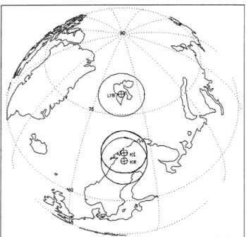
Fig. 1. Location of the three FPIs at Longyearbyen, Kilpisjarvi and
Kiruna. The circles surrounding each site indicate the field of view of the FPI for the zenith angle of observation used with each FPI. This assumes a peak emission height of 240 km for the 630 nm emission and a zenith angle of 60◦which gives a circle with radius 416 km.
2 The instruments
The Atmospheric Physics Laboratory has operated FPIs for many years and has had instruments deployed at 3 sites in Scandinavia for a large part of the past 20 years (e.g. Rees et al., 1989). Observation of the OI emission at 630 nm allows the determination of the neutral winds and temperatures of the upper thermosphere. The combination of data from the 3 sites can be used to see the large-scale flow behaviour of the high-latitude thermosphere, from polar cap regions to the auroral oval. The two auroral sites are at Kiruna, Sweden (67.8◦N, 20.4◦E) and Kilpisjarvi, Finland (69.2◦N, 20.8◦E). The polar cap site is on the island of Svalbard, at Longyear-byen (78.2◦N, 15.6◦E). Figure 1 shows the location of these three FPIs. The circles surrounding each site indicate the fields of view of the FPIs for the zenith angle of observa-tion used with each instrument. This assumes a peak emis-sion height of 240 km for the 630 nm emisemis-sion, which cor-responds to a horizontal radius of 416 km for a zenith angle of 60◦. Originally, all three FPIs used this angle until the zenith angle of the Kiruna FPI was changed to 45◦ (which corresponds to a horizontal radius of 240 km) at the end of December 1990, in order to improve the geometry of exper-iments requiring co-located observations with the EISCAT radar.
The FPI has a 1◦field of view. Observations are made by way of a tilted mirror of 7 viewing directions plus a neon cal-ibration lamp to monitor the instrument stability. The stan-dard cycle of observations are: North, North-East, East,
Cal-Fig. 2. Average large-scale thermospheric wind flow at high-latitudes (60◦N–80◦N) for geomagnetically quiet conditions (0≤ Kp < 2). Neutral gas motion is dominated by pressure gradients set up by solar heating, thus the flow is mainly anti-sunward.
Fig. 3. Average large-scale thermospheric wind flow at high-latitudes (60◦–80◦N) for moderately active geomagnetic conditions (2 ≤ Kp < 5). The modifying influence of the plasma is appar-ent in several respects. A clockwise cell corresponding to the dusk cell of the high-latitude electric field can be seen, centred at about 1600UT and between 70◦–75◦N. Between 56◦–70◦N the flow is westward before 2100UT and eastward afterwards. The Harang Discontinuity is fairly distinct. There is little evidence of the dawn cell.
ibration Lamp, South, Zenith, West and North-West. The integration time has generally been 1 minute for each direc-tion. Thus, a complete cycle takes 15 minutes when includ-ing the time taken for the mirror to rotate to each new po-sition. The average separation of the zenith and calibration lamp peaks over the complete night is calculated and used as an offset to the calibration lamp peak. This is used as the zero Doppler shift baseline from which the Doppler shifts and consequently wind speeds in each of the line-of-sight di-rections can be deduced. This procedure is discussed in more detail in Sect. 4.1.1 and also in Aruliah and Rees (1995).
The wind vectors shown in this paper (i.e., Figs. 2–5) are derived by vectorially combining 3 adjacent line-of-sight mea-surements, such as NW, N and NE, together with a mean vec-tor calculated from a complete cycle of measurements. Since the 3 line-of-sight measurements are not contemporaneous,
A. L. Aruliah and E. Griffin: Evidence of meso-scale structure in the high-latitude thermosphere 39
Fig. 4. (a) EISCAT radar ion velocities for the 24 hour period
be-ginning at 1200UT on the 15thDecember 1987. For clarity, only velocities for each hour are plotted. (b) Labelled regions common to both the ion and neutral flows are superposed on the ion velocities for comparison with Fig. 5.
the procedure is to use linear interpolation of the actual mea-surements to calculate line-of-sight winds at 15 minute in-tervals (e.g. at 0000UT, 0015UT, 0030UT . . .. etc.). The interpolated line-of-sight winds are subsequently combined as described.
The overall mean vector is found by fitting a sinusoid to all the interpolated line-of-sight measurements for a given 15 minute interval. The assumption made here is that there is a uniform wind field over the whole field of view. This is patently not true which is why the 3 line-of-sight mea-surements are also used to look for non-uniform flow on the meso-scale. The line-of-sight measurements are presumed to lie on the circumference of a circle as shown in Fig. 1. The combination of 3 adjacent line-of-sight measurements means that the resultant vector is smoothed only over the time taken to make the 3 measurements, i.e. a period of 5 minutes for an integration time of 1 minute. The mean vector represents a 15 minute smoothing effect, but its contribution is only a quarter of the total. The purpose of its inclusion is to allow for a continuity of wind flow over the whole field of view. This is just one of several methods used to derive vectors from successive line-of-sight measurements (e.g., Burnside et al., 1981; Meriwether et al., 1987; Greet et al., 1999).
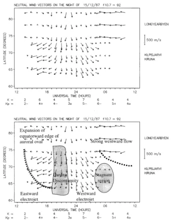
Fig. 5. (a) Neutral winds observed on the night of 15–16 December
1987 with FPIs at Kiruna, Kilpisjarvi and Longyearbyen. (b)
Labelled regions common to both the ion and neutral flows are superposed on the neutral winds for comparison with Fig. 4.
3 Large-scale behaviour of high-latitude wind
The sets of data presented in Sect. 3 as Figs. 2, 3 and 5 il-lustrate the large-scale wind flow from the polar cap to the auroral oval as seen by the FPIs at Kiruna, Kilpisjarvi and Longyearbyen. This gives a context for the meso-scale flows that will be described in Sect. 4. Section 3.1 discusses the be-haviour of average winds for geomagnetically quiet and mod-erately active conditions to indicate the important controlling factors and the subsequent direction of the wind flow. This is followed in Sect. 3.2 by a comparison between EISCAT plasma velocities and FPI winds from a single moderately active night.
One of the major issues of concern is a commonly used simplification when calculating Joule heating that sets the neutral wind speed to zero. The equation for Joule heating should beR σpE0dz, where σpis the Pedersen conductivity, E0=E + U × B is the electric field in the neutral frame of
reference, E is the electric field in the Earth’s frame of refer-ence and U is the neutral wind at height z. The Joule heating equation can be simplified to ER σpdz, by assuming U = 0
at all heights, which further simplifies to EP
p, where P
p
is the height integrated conductivity. This is usually justified by reasoning that the neutral winds are very variable over
the height region concerned (i.e., greater than 90 km), and that there are very few measurements available. (Also, the height integrated conductivity can be directly measured by radar and ionosonde while deriving a height profile of σpis a
more involved process.) However, the figures in Sect. 3 show that the large-scale neutral wind flows at 240 km altitude are not insignificant and consequently should not be ignored. The same applies to lower thermosphere winds as can be seen, for example, in those deduced from EISCAT radar mea-surements by Kirkwood et al. (1996). Furthermore, Thayer (1998) has estimated that the inclusion of neutral winds when calculating the height integrated Joule heating made a differ-ence of up to 400% for the two 24-hour periods of data from the Sondrestrom incoherent scatter radar that he studied.
The inertia of the neutral atmosphere also introduces an added dimension which Aruliah et al. (1999) have termed the “geomagnetic history”. This means that the geomagnetic activity conditions of the previous 3–6 hours will affect the neutral wind, resulting in a considerable difference in the mo-mentum transfer and Joule heating. Thus, the current level of geomagnetic activity is not a sufficient indicator of the be-haviour expected.
3.1 Average winds: Dependence on geomagnetic activity Figures 2 and 3 show average neutral wind vectors for a 24-hour period centred on 0000UT, between latitudes 60◦– 82◦N. The data are long-term averages from the FPI databa-ses of winds at Kiruna and Longyearbyen during solar min-imum (F10.7 < 150) which are sorted by geomagnetic ac-tivity. Figure 2 shows average wind vectors for geomag-netically quiet (0 ≤ Kp < 2) conditions and Fig. 3 for moderately active (2 ≤ Kp < 5) conditions. The number of nights contributing to the average wind values observed at Longyearbyen is 54 ± 15 and 41 ± 14 for the quiet and moderately active conditions, respectively. These were ob-tained from 4 winters of observations. The number of nights from 6 winters of observations at Kiruna is 26 ± 13 and 69
±41 for the quiet and moderately active conditions, respec-tively. The “±” range of dates reflects the seasonal depen-dence of the observing period because the FPI is only able to take images during the hours of darkness. At Kiruna, for example, the observing period ranges from about 4 hours at the beginning and end of the observing season (September and April, respectively) to around 17 hours in mid-winter. Consequently, the largest data contribution coming from all the winter months is around local midnight, while the early evening and morning hours can only be observed in the mid-dle of winter.
The average winds for geomagnetically quiet conditions (Fig. 2) demonstrate that solar heating is the dominant driv-ing force for Kp < 2. The flow is generally antisunward over the polar cap. Thus, above 75◦N, the flow is equator-ward (southequator-ward) between 1600–0300UT and poleequator-ward for a few hours around 1200UT. The average wind vector ro-tates smoothly between poleward and equatorward flow di-rections. Meanwhile, in the auroral region between 65◦–
72◦N, the afternoon vectors (1500–1800UT) are eastward,
rotating to south at 0200UT and then west after 0400UT. Increased geomagnetic activity strongly modifies the neu-tral wind flow because ion-neuneu-tral coupling becomes more effective owing to the increase in electron density through particle precipitation at these latitudes. The increased strength of ion drag diverts the neutral flow from the pressure-gradient driven antisunward direction to a flow pattern that more clo-sely matches the two cell convection pattern of the high-latitude electric field which the ions follow. This is clearly seen in Fig. 3. A clockwise flow centred on 1600–1800UT and 70◦–75◦N corresponds to the dusk cell of the high-lati-tude electric field. The Harang Discontinuity, which sepa-rates the westward electrojet from the eastward electrojet, is apparent in the change in the neutral wind flow at around 2100UT. However, the dawn cell does not appear in the neu-tral winds. Fuller-Rowell and Rees (1984) have interpreted this as being due to the Coriolis force that favours the clock-wise motion of the neutral flow in the dusk cell in the North-ern Hemisphere. The direction of this force on the neutrals constrains the particles within the cell so that momentum is built up. Meanwhile, the Coriolis force throws the gas par-cel out of the region of the anticlockwise plasma flow of the dawn cell, so the anticlockwise flow cannot be maintained for the neutral circulation.
There is a close correspondence between the geomagnetic activity Kp index and the Bz component of the
Interplane-tary Magnetic Field (IMF). This means that a similar trend in the large scale wind flow can be expected when com-paring average winds sorted according to BZ-negative
val-ues (“open magnetosphere” resulting in geomagnetically ac-tive conditions) with average winds sorted according to small
BZ-positive values (“closed magnetosphere” resulting in
ge-omagnetically quiet conditions). The BY component of the
IMF modifies the relative size of the dawn and dusk cells of the high-latitude electric field (e.g. Weimer, 1995). As a result, the sizes of both the BY and BZ components have
a significant effect on the ion-neutral coupling relationship, and consequently, the neutral winds, as has been shown by Meriwether and Shih (1987) and Killeen et al. (1995). The next section shows that the more dynamic the situation for an individual period of observation, the smaller the scale size of the neutral wind response to magnetospheric driving. 3.2 A particular night 15–16 December 1987: Comparison
with ion flows
A single moderately active night, 15–16 December 1987, has been chosen from the winter of 1987–1988, when all three FPIs were operating and there were several nights with sig-nificant periods of cloudless skies at all the sites. Cloudless skies are necessary because the presence of clouds causes scattering of the emission resulting in directional informa-tion being lost. In addiinforma-tion, the EISCAT radar was operat-ing in CP-3 mode which is a scannoperat-ing mode where the radar antenna moves along the magnetic meridian pausing at 13 different elevation angles, with a cycle period of about 30
A. L. Aruliah and E. Griffin: Evidence of meso-scale structure in the high-latitude thermosphere 41 minutes. The data cover a range of latitudes between 64◦–
73◦N.
Figures 4a and 5a show the ion velocities and neutral winds, respectively, observed on this night. Superficially the two sets of data have only a passing resemblance. However, dis-tinct regions of matched behaviour may be identified as shown by comparison of Figs. 4b and 5b. These are the same plots as Figs. 4a and 5a, but with the superposition of labelled re-gions. It is the close correspondence of the behaviour of the two datasets that is being highlighted in this section, to show that the neutral winds can indeed be significantly variable un-der moun-derately active conditions when ion-neutral coupling is strong.
The ion velocities shown in Fig. 4 are measured at a con-stant height of 280 km. The data are sorted into 5 bins, each covering a latitude range of 2◦. There are several features to
be pointed out. The Kp index for the period 1200–1500UT is 2− and then it rises to 4+ for the next 3 hours. It re-mains moderately high for the rest of the 24 hour period. Between 1200 and 1800UT the equatorward edge of the au-roral oval can be identified as the separation between small and large ion velocities. It is seen to move from about 71◦N at 1300UT to 65◦N between 1400 and 1800UT. The ion flow in the auroral oval is strongly south-westward, followed by a clear switch to a north-eastward flow. This occurs at dif-ferent times for difdif-ferent latitudes. Thus, at 72◦N, the switch occurs at 2000UT and at 65◦N, it is 2 hours later. This is broadly consistent with the region of the Harang Discontinu-ity.
Figure 5 shows the equivalent neutral winds for this night. The Longyearbyen FPI covers a latitude range of about 75◦–
83◦ N, and the Kiruna and Kilpisjarvi FPIs cover a range
of about 64◦–73◦N. Before 1500UT the winds observed at
Kiruna and Kilpisjarvi are small, north-easterly, and typical of quiet conditions as shown in Fig. 2. This indicates that the winds are driven by the pressure gradient and that the auroral oval is poleward of these sites. Meanwhile, the winds ob-served at Longyearbyen are strongly westward, which means that the pressure gradient is not the dominant driving force in the polar cap despite a quiet geomagnetic index value of
Kp =2. Comparison with Fig. 4 shows that the ion flows above 70◦N at 1300UT and 1400UT are westward and south-westward, respectively, which is compatible with the neutral flow. At 1600UT there is a sharp acceleration of the neutral atmosphere above Kiruna and Kilpisjarvi to speeds of around 300 m/s in a west-southwest direction. This corresponds to the extension of the equatorward edge of the auroral oval to the latitude of Kiruna as indicated by the sharp rise of the Kp index to Kp = 4+. (The local K index for Kiruna, which is also given in Fig. 5, rises to K = 6 for the interval 1500– 1800UT.)
The Harang Discontinuity is clearly defined between 2000– 2300UT. The westward ion flow in the dusk sector is far more successful in diverting the neutrals than the eastward ion flow due to the Coriolis force, as explained earlier. Thus, while the neutral winds flow parallel to the ions between 1600– 2100UT, from about 2200–0500UT, the two flows are almost
orthogonal.
In the region defined by 0400–0700UT and 64◦–70◦N, the
ion flow appears to be confused. This may be understood if, instead of considering the abscissa as a time axis, it is consid-ered a longitudinal axis, in which case, this region is a con-fluence of two strong flow regimes: a strong northeast flow prior to 0400UT and a strong southwest flow after 0800UT. The neutral winds at Kiruna and Kilpisjarvi consequently can become very small from 0400UT until the end of the FPI ob-serving period.
There is a further compatibility between the radar and FPI observations. The CP-3 radar observations extend only to 73◦N, which is south of the southernmost observing position of the Longyearbyen FPI. The radar first sees large westward ion flows at 0800UT at 73◦N. An hour later, fast flows are seen at 64◦N too. However, the neutral wind observed at
Longyearbyen turns strongly westward between 0400–0500 UT. The magnitude of the neutral wind is only about 270 m/s compared with 700 m/s ion flows. The implication from the behaviour of the neutral winds at Longyearbyen is that the ionospheric forcing started at very high-latitudes before mov-ing equatorward.
4 Meso-scale behaviour of high-latitude winds
Having described the large-scale behaviour of the neutral at-mosphere, Sect. 4 presents the evidence for meso-scale be-haviour seen by FPIs in northern Scandinavia. The inertia of the neutral atmosphere on the large-scale is acknowledged, but on the medium scale there can be a rapid and localised response to ionospheric forcing. This is likely to have a significant influence on ion-neutral interactions and the en-ergy budget. Most ground-based experiments make mea-surements over a range of hundreds, rather than thousands, of kilometres and so this is an important consideration.
There have been regular attempts to increase the spatial and temporal resolution of measurements of the thermosphere in the past. However, this is possibly driven as much by the enthusiasm for pushing instrumental capabilities to their lim-its as for the searching for meso-scale structure. Thus, the original single photomultiplier detectors for the earliest FPIs used in upper atmospheric research are being replaced by two-dimensional arrays of photon counting devices or, more recently, CCDs. This allows much greater light throughput, and consequently, a decrease in the integration times and in-crease in temporal resolution. The results presented in this section are the consequences of these advances and are sep-arated into observations of meso-scale spatial and temporal variations.
4.1 Evidence of medium spatial scale structure 4.1.1 Direct measurements of neutral winds by
narrow angle imagers – FPIs
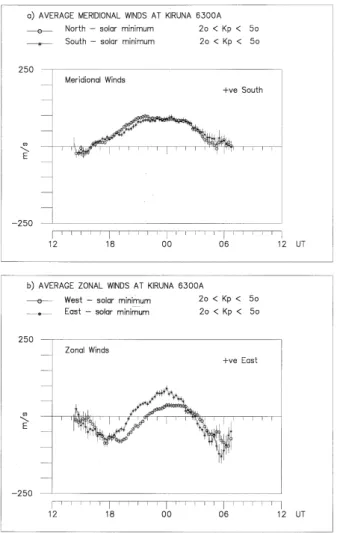
Figure 6 compares average meridional wind observations made to the North and South (Fig. 6a) and zonal wind
ob-Fig. 6. Comparison of the (a) average meridional and (b) average
zonal components of the neutral winds observed to the North and South, and to the East and West of Kiruna, respectively. The peak emission height of the 630 nm emission is around 240 km. As a re-sult a horizontal distance of over 800 km separates the observations in opposite directions.
servations to the East and West (Fig. 6b) of Kiruna. The av-erage winds from Kiruna are calculated using moderately ac-tive (2 ≤ Kp < 5) data from the 5 winters between Septem-ber 1983 and April 1988. This is a period of solar minimum, when the solar flux index was in the range 80 < F10.7<120. The average number of nights contributing to each 15 minute interval is 69±41 and the standard error of the mean for the average wind speeds is ±2 m/s. There is a significant gradi-ent in the wind field, with the largest consistgradi-ent difference be-ing about 50 m/s in the zonal winds durbe-ing the period 1900– 0200UT. Between 1800UT and 0600UT the magnitude of the zonal wind component observed to the east is up to 100% larger than to the west. Furthermore, the position of the Ha-rang Discontinuity, where the zonal wind changes from west-ward to eastwest-ward, is observed nearly 2 hours later in the west pointing direction.
A much smaller, though statistically significant, difference between the observations to the North and South of Kiruna
can also be seen in the average meridional winds. The dif-ference is in the period 1900– 2100UT. Although not shown here, it should noted that the average meridional winds at so-lar maximum show a difference over a more extended period of 1800–2300UT.
In order to put these gradients in context, it should be pointed out that the peak emission height of the 630 nm emis-sion is around 240 km which means that diametrically oppo-site observations made at a zenith angle of 60◦are separated by a horizontal distance of over 800 km. Conventional theory would expect the wind to be fairly uniform over this field of view. This assumption has been commonly used to calculate the Doppler shifts from FPI measurements. This is because there is, as yet, no convenient laboratory source of 630 nm to provide a zero Doppler shift baseline. Consequently, the simplest procedure has been to average the blue shift seen in one direction, with the red shift seen in the opposite direction and assume a uniform wind.
A more sophisticated procedure, which is used here, is to calculate the average separation throughout each night of the 630 nm emission peak observed in the vertical direction from a neon calibration lamp peak. The assumption is made that the average zenith wind through the night is zero, i.e., there is no net up- or down-welling owing to the conservation of mass. The average separation is then used as an offset value that is added to the calibration lamp emission peak to create a zero Doppler shift baseline. All the 630 nm measurements are then compared with this baseline to calculate the Doppler shifts and subsequently the line-of-sight wind measurements. There are limitations to this method, as shown by Aruliah and Rees (1995), because the assumption of no net up- or down-welling applies to a full 24 hour period, while FPI observa-tions are limited to nighttime hours. Furthermore, average vertical wind data show that there are Kp-dependent, sea-sonal and solar cycle trends in the behaviour of the vertical winds. As a result it was suggested that the baseline error associated with this method is a systematic error of around 5 m/s for geomagnetically quiet conditions, and 10–20 m/s for active conditions. However, since this systematic error is less than the gradients seen in the meridional and zonal av-erage winds shown in Fig. 6, it is reasonable to suggest that the gradients reveal a persistent meso-scale structure.
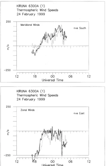
An example of the dynamic variability in the gradient for an individual night is shown by the neutral winds observed by the Kiruna FPI on the night of the 24th February 1999 (Fig. 7). The geomagnetic activity was, in general, mod-erately active before 2100UT, i.e., Kp = 2 to 3, and quiet afterwards; Kp ∼ 1, except for Kp = 4−during the period
0300–0600UT. The error bars for the wind speeds are around
±25 m/s for this night. As explained above, the offset has been chosen so that the vertical wind component averages to zero over the 12 hours of observation. Any attempt to choose an offset to minimise the gradient in the horizontal compo-nent will result in a persistent upwelling or downwelling over the 12 hour period, which is not a physically justifiable pre-sumption. What is noteworthy is that there are random and non-repetitive variations in the gradient which are indicative
A. L. Aruliah and E. Griffin: Evidence of meso-scale structure in the high-latitude thermosphere 43
Fig. 7. Comparison of the (a) meridional and (b) zonal components
of the neutral winds observed to the North and South, and to the East and West of Kiruna, respectively, on the night of the 24thFebruary 1999. The error bars have been omitted for clarity. The errors in the wind measurements are around ±25 m/s. The geomagnetic ac-tivity was variable – in general moderately active before 2100UT and quiet afterwards. The figure illustrates the dynamic variability of the gradient in the winds over a 500 km diameter field of obser-vation.
of even smaller-scale features that would be smoothed out of the long-term averages shown elsewhere. A recent paper by Greet et al. (1999) shows similar gradients in the wind fields seen during individual nights by two FPIs at the Mawson and Davies stations in Antarctica although they use a different analysis technique.
4.1.2 Direct measurements of neutral winds by wide-angle imagers
The earliest optical instruments that imaged the whole sky simultaneously were deployed by the Atmospheric Physics Laboratory, UCL, in Kiruna in 1982 (Batten et al., 1988). These were called Doppler Imaging Systems and were
ba-sically field-widened FPIs. The etalon had a fixed gap size. Thus, the spatial resolution was determined by the number of circular fringes imaged, which in turn was limited by the detector resolution. Subsequently, a small number of other groups built similar instruments (e.g. Biondi et al., 1995). However, the analysis of the data is very time-consuming ow-ing to the problems of image distortion by aberrations of the lens or detectors. The accuracy required to image the fringes puts stringent demands on the positional linearity and stabil-ity of the imaging detector. Large intensstabil-ity gradients also distort the circular fringe profile, which is an important con-sideration in auroral regions where there are highly localised regions of particle precipitation. As a result, there are only “first results” papers available.
More recently, Conde and Smith (1997) have achieved a radical improvement in FPI research. They have built a Scan-ning Doppler Imager (SDI) which is a FPI with an etalon that has a variable gap size. The gap size is scanned through a free spectral range so that each pixel of the detector becomes self- calibrated. Thus, distortions from the instrument and intensity variations are limited to the region covered by the pixel. The instrument effectively acts like an array of photo-multipliers. The initial results of all these field-widened in-struments show considerable structure with scale sizes of the order of 100’s of kilometres (e.g. Conde and Smith, 1998).
4.2 Evidence of medium temporal scale structure 4.2.1 Derived neutral winds from plasma velocities Figure 8 shows a comparison between neutral winds derived from ion velocities measured by the EISCAT radar on the 21stJanuary 1990 using the assumption of diffusive equilib-rium, and neutral winds measured directly with the Kiruna FPI (Davis, 1993). It should be pointed out that Davis et al. (1995) showed that the derivation can be successful at high-latitudes only under very particular conditions that may be tested statistically. The statistical test then becomes a con-dition adcon-ditional to that of restricting the Kp index to low values, i.e., geomagnetically quiet conditions. The example here satisfies these conditions and therefore probably satis-fies the assumption of diffusive equilibrium. Thus, the agree-ment between the radar-derived and FPI winds is good. How-ever, small-scale temporal variations are evident in the neu-tral winds derived from the ion flows (solid line), but those measured by the FPI are smooth (dashed line). This could suggest that the higher time resolution radar measurements show real temporal variations in the thermosphere that have been missed by the FPI.
4.2.2 Direct measurements of neutral winds and tempera-tures by an FPI
In January 1996 the second FPI in Kiruna was upgraded by the installation of a new Intensified CCD detector. There was a dramatic improvement in the time resolution from 120 sec-onds integration time with the old Imaging Photon Detector
Fig. 8. Comparison of meridional winds directly measured by the
FPI at Kiruna with those derived from EISCAT plasma velocities using the assumption of diffusive equilibrium. Data from the 21st January 1990 show that under very particular conditions that may be tested statistically the derivation can be successful (from Davis, 1993).
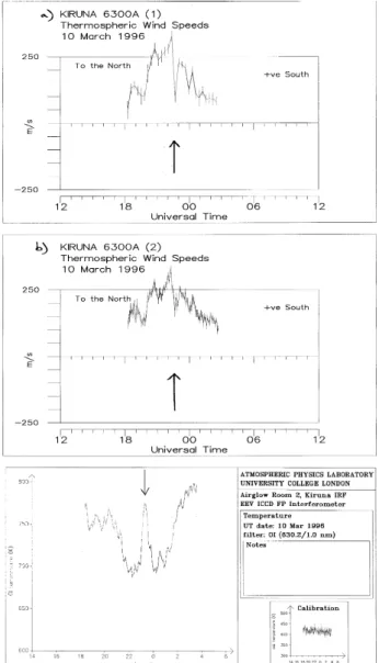
(IPD) to 15 seconds with the ICCD. Figures 9a and 9b com-pare meridional wind data observed on the 10thMarch 1996 by the two FPIs. There is a feature in the meridional wind component just before 2300UT that is marked with an arrow on the figure. The wind speed drops by 150 m/s and then rises again over a short period of only 40 minutes. The feature may have been suspect as an outlier in the readings for the FPI us-ing an IPD, since there is only one data point, but it appears in the high resolution ICCD FPI measurements with interme-diate data points to confirm the rapid change. The rapid drop in wind speed is matched by a simultaneous measurement of a large rise and fall in temperature of around 70 K as shown in Fig. 9c. It is worth pointing out that the neutral winds un-der these moun-derately active and variable conditions could not have been derived from ion velocity measurements because the assumption of diffusive equilibrium is not appropriate.
Unfortunately, the phosphor used as the intensifier in the ICCD detector was found to have an undesirably long decay time. An emission peak could still be seen up to 2 minutes af-ter the exposure. Thus, contamination from previous viewing directions could distort the images, depending on what their relative intensities were. This is why the wind measurements made with the ICCD do not match the IPD measurements precisely. As a consequence, bare CCD detectors which re-quire longer integration times were chosen for subsequent FPIs that were built. The time resolutions of the bare CCDs in current use are similar to that of the IPDs and therefore, there is no time advantage. However, the advantage of the bare CCD over the IPD is the lack of image distortion which allows reliable measurements of the Doppler broadening and consequently neutral temperature. There are plans for the use of a novel photon counting CCD detector for future work at higher time-resolutions.
Fig. 9. Comparison of the meridional component of thermospheric
winds measured on the 10thMarch 1996 at Kiruna with a FPI using
(a) an Imaging Photon Detector (IPD) which has an integration time
of 120 seconds and (b) an Intensified CCD detector (ICCD) which requires only a 15 second integration time. Note the sharp drop and rise in wind speed between 2200UT and 2300UT. Only one data point marks this in (a) and the datum may have been disregarded as an outlier, however, the high time resolution of the ICCD shows in Fig. 9b that this is a real feature. (c) Thermospheric temperatures measured using the new ICCD detector show a rapid rise and fall in temperature between 2200UT and 2300UT that corresponds with the rapid drop and rise in wind speed shown in (a) and (b).
5 Comparison with model simulations
The general climatology of the neutral atmosphere is well known and can be well modelled. However, there are certain anomalies, most importantly, existing models underestimate Joule heating and overestimate momentum transfer through ignoring random fluctuations in plasma velocities, which is a small or meso-scale phenomenon. For example, Fig. 10
A. L. Aruliah and E. Griffin: Evidence of meso-scale structure in the high-latitude thermosphere 45
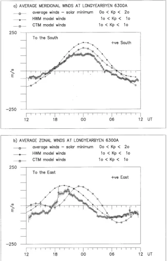
Fig. 10. Comparison of average meridional neutral winds for
ge-omagnetically quiet conditions (0 < Kp < 2) at solar minimum (mean F10.7 = 100) measured with a FPI at Longyearbyen with theoretical CTIM model winds and empirical HWM model winds simulated by using Kp = 1 and F10.7 = 73. There is a severe overestimation of the wind magnitudes by the model, which prob-ably arises from an overestimation of momentum transfer through ignoring meso-scale fluctuations.
compares the FPI average meridional and zonal neutral wind component for Longyearbyen at solar minimum with winds calculated by the theoretical CTIM model (Fuller-Rowell et al., 1996) and the empirical Horizontal Wind Model (Hedin et al., 1991). The FPI average wind data were obtained dur-ing the winters of 1986–1987, 1987–1988, 1992–1993, 1993– 1994 and 1997–1998. The average solar flux level for the FPI winds is F10.7=100 and the mean Kp value is 1. It is appar-ent that standard steady state simulations from both models systematically overestimate the magnitude of the winds de-spite using much quieter input parameters, i.e., F10.7 = 72 and Kp = 10. This shows that great care must be taken when using models to determine ion-neutral coupling param-eters for individual observing periods when there are no di-rect measurements of the neutral atmosphere.
The spatial resolution of current models is too poor at
high-latitudes to investigate meso-scale structure and consequently attempt to allow for fluctuations. For example, the CTIM model has a spatial grid size that is 2◦latitude and 18◦
longi-tude. In terms of distance in kilometres, this is equivalent to approximately 100 km by 750 km for a latitude of 68◦. This is being dealt with by using nested grid models such as the TING model (Wang et al., 1999). However, with the vastly increased capabilities of modern computers two decades af-ter the first use of these models, it is likely that spatial and temporal resolution will improve dramatically in the future.
A more important concern is that the assumptions about the neutral response are reinforced through their use in mod-els if it is not acknowledged that the modmod-els are only as good as their assumptions. This applies also to where neutral pa-rameters are derived from ionospheric measurements. Fur-thermore, these assumptions require reassessment to keep up with the considerable improvements in instrumental and model capabilities.
6 Conclusions
It is generally assumed that the thermosphere smoothes out the dynamic ionospheric forcing in a predictable manner. The large-scale wind flows observed by a chain of three FPIs, from the polar cap to the auroral region, show a smoothly varying wind field as a first order assumption over a range of a few hundred kilometres. However, data presented here and elsewhere shows significant spatial structure on the meso-scale. This indicates a need for the deployment of more all-sky Fabry-Perot systems such as the one pioneered by Conde and Smith (1997). In addition, increased time resolution for the FPI measurements has shown variation over a scale of tens of minutes. It is proposed that increasing the time reso-lution of ionospheric measurements to mere seconds, or less, demands that the neutral gas behaviour be investigated at near similar resolutions, at least to determine the limitations of the assumptions that are currently used. (Resolutions of several seconds are possible using current technology.) Oth-erwise, calculations of parameters such as momentum trans-fer and Joule heating are likely to be seriously compromised.
Acknowledgements. The research is supported by grants from
PPARC. The authors gratefully acknowledge the considerable amount of work undertaken by the FPI team, in particular Ian McWhirter, at the Atmospheric Physics Laboratory, UCL, in de-signing, constructing and deploying the FPIs for the Scandinavian network. Thanks also to our colleagues at the remote sites for their assistance in maintaining the instruments. Jackie Schoendorf kindly accessed the EISCAT and CTIM model databases for these com-parisons. The Kp indices come from the World Data Centre C1 at the Rutherford Appleton Laboratory. The EISCAT radar facil-ity is an international association supported by the research coun-cils of Finland (SA), France (CNRS), Federal Republic of Germany (MPG), Japan (NIPR), Norway (NAVF), Sweden (NFR) and the United Kingdom (PPARC).
Topical editor D. Murtagh thanks J. W. Meriwether and M. Conde for their help in evaluating this paper.
References
Aruliah, A. L. and Rees, D., The trouble with thermospheric verti-cal winds: Geomagnetic, seasonal and solar cycle dependence at high latitudes, J. Atmos. Terr. Phys, 57, 597–609, 1995. Aruliah, A. L., Mueller-Wodarg, I. C. F., and Schoendorf, J., The
consequences of geomagnetic history on the high-latitude ther-mosphere and ionosphere: Averages, J. Geophys. Res., 104, 28073–28088, 1999.
Batten, S. and Rees, D., Thermospheric winds in the auroral oval: Observations of small scale structures and rapid fluctuations by a Doppler imaging system, Planet. Space Sci., 38, 675–694, 1990. Biondi, M. A., Zipf, M. E., Sipler, D. W., and Baumgardner, J. L., All-sky Doppler interferometer for thermospheric dynamics studies, Applied Optics, 34, 1647–1654, 1995.
Burnside, R. G., Herrero, F. A., Meriwether Jnr, J. W., and Walker, J. C. G., Optical observations of thermospheric dynamics at Arecibo, J. Geophys. Res., 86, 5532–5540, 1981.
Conde, M. and Smith, R. W., Phase compensation of a separation scanned, all-sky imaging Fabry-Perot spectrometer for auroral studies, Appl. Optics, 36, 5441–5450, 1997.
Conde, M. and Smith, R. W., Spatial structure in the thermospheric horizontal wind above Poker Flat, Alaska, during solar mini-mum, J. Geophys. Res, 103, 9449–9471, 1998.
Davis, C. J., The interaction between the thermosphere and iono-sphere at high latitudes, Ph. D. thesis, University of Southamp-ton, 1993.
Davis, C. J., Farmer, A. D., and Aruliah, A. L., An optimised method for calculating the O(+)-O collision parameter from aero-nautical measurements, Ann. Geophys., 13, 541–550, 1995. Farmer, A. D., Winser, K. J., Aruliah, A., and Rees, D.,
Ion-Neutral Dynamics: Comparing Fabry-Perot measurements of neutral winds with those derived from radar observations, Adv. Space Res., 10, 6281–6286, 1990.
Fuller-Rowell, T. J., and Rees, D., Interpretation of an anticipated long-lived vortex in the lower thermosphere following simulation of an isolated substorm, Planet. Space Sci., 32, 69–85, 1984. Fuller-Rowell, T. J., Rees, D., Quegan, S., Moffett, R. J., Codrescu,
M. V., and Millward, G. H., A coupled thermosphere-ionosphere model (CTIM), STEP Handbook, ed. R. W. Schunk, 1996. Greet, P. A, Conde, M. G., Dyson, P. L., Innis, J. L., Breed, A.
M., and Murphy, D. J., Thermospheric wind field over Mawson
and Davis, Antarctica: Simultaneous observations by two Fabry-Perot spectrometers of 630 nm emission, J. Atmos. Solar Terr. Phys., 61, 1025–1045, 1999.
Hedin, A. E., Biondi, M. A., Burnside, R. G., Hernandez, G., John-son, R. M., Killeen, T. L., Mazaudier, C., Meriwether, J. W., Salah, J. E., Sica, R. J., Smith, R. W., Spencer, N. W., Wickwar, V. B., and Virdi, T. S., Revised Global Model of Thermospheric winds using satellite and ground-based observations, J. Geophys. Res., 96, 7657–7688, 1991.
Killeen, T. L., Won, Y.-I., Niciejewski, R. J., and Burns, A. G., Up-per Thermosphere Winds and TemUp-peratures in the Geomagnetic Polar Cap: Solar cycle, geomagnetic activity and IMF dependen-cies, J. Geophys. Res., 100, 21327–21342, 1995.
Kirkwood, S., Lower thermosphere mean temperatures, densities, and winds measured by EISCAT: Seasonal and solar cycle ef-fects, J. Geophys. Res., 101, 5133–5148, 1996.
Meriwether, J. W., Heppner, J. P., Stolarik, J. D., and Wescott, E. M., Neutral winds above 200 km at high latitudes, J. Geophys. Res., 78, 6643–6661, 1973.
Meriwether, J. W. and Shih, O., On the nighttime signatures of ther-mospheric winds observed at Sondrestrom, Greenland, as corre-lated with interplanetary magnetic field parameters, Ann. Geo-physicae, 5A, 329–336, 1987.
Meriwether, J. W., Killeen, T. L., McCormac, F. G., Burns, A. G., and Roble, R. G., Thermospheric winds in the geomagnetic polar cap for solar minimum conditions, J. Geophys. Res., 93, 7478– 7492, 1988.
Rees, D., McWhirter, I., Aruliah, A., and Batten, S., Upper at-mospheric wind and temperature measurements using imaging Fabry-Perot interferometers, Chapter 7, WITS Handbook of ex-perimental techniques, 2, 188–223, edited by C. H. Liu, 1989. Thayer, J. P., Height-resolved Joule heating rates in the high-latitude
E-region and the influence of neutral winds, J. Geophys. Res., 103, 471–487, 1998.
Wang, W., Killeen, T. L., Burns, A. G., and Roble, R. G., A high res-olution three-dimensional, time-dependent, nested grid model of the coupled thermosphere-ionosphere, J. Atmos. Sol. Terr. Phys., 61, 385–397, 1999.
Weimer, D. R., Models of high-latitude electric potentials derived with a least error fit of spherical harmonic coefficients, J. Geo-phys. Res., 100, 19595–19607, 1995.