HAL Id: hal-02969178
https://hal.archives-ouvertes.fr/hal-02969178
Submitted on 26 Oct 2020
HAL is a multi-disciplinary open access
archive for the deposit and dissemination of
sci-entific research documents, whether they are
pub-lished or not. The documents may come from
teaching and research institutions in France or
abroad, or from public or private research centers.
L’archive ouverte pluridisciplinaire HAL, est
destinée au dépôt et à la diffusion de documents
scientifiques de niveau recherche, publiés ou non,
émanant des établissements d’enseignement et de
recherche français ou étrangers, des laboratoires
publics ou privés.
power plants with the Copernicus Anthropogenic CO2
Monitoring (CO2M) mission
Gerrit Kuhlmann, Grégoire Broquet, Julia Marshall, Valentin Clément, Armin
Löscher, Yasjka Meijer, Dominik Brunner
To cite this version:
Gerrit Kuhlmann, Grégoire Broquet, Julia Marshall, Valentin Clément, Armin Löscher, et al..
De-tectability of CO2 emission plumes of cities and power plants with the Copernicus Anthropogenic CO2
Monitoring (CO2M) mission. Atmospheric Measurement Techniques, European Geosciences Union,
2019, 12 (12), pp.6695-6719. �10.5194/amt-12-6695-2019�. �hal-02969178�
https://doi.org/10.5194/amt-12-6695-2019 © Author(s) 2019. This work is distributed under the Creative Commons Attribution 4.0 License.
Detectability of CO
2
emission plumes of cities and power plants with
the Copernicus Anthropogenic CO
2
Monitoring (CO2M) mission
Gerrit Kuhlmann1, Grégoire Broquet2, Julia Marshall3, Valentin Clément4,5, Armin Löscher6, Yasjka Meijer6, and Dominik Brunner1
1Empa, Swiss Federal Laboratories for Materials Science and Technology, Dübendorf, Switzerland 2Laboratoire des Sciences du Climat et de l’Environment, LSCE/IPSL, CEA-CNRS-UVSQ,
Université Paris-Saclay, Gif-sur-Yvette, France
3Max Planck Institute for Biogeochemistry (MPI-BGC), Jena, Germany
4Center for Climate Systems Modelling (C2SM), ETH Zurich, Zurich, Switzerland 5MeteoSwiss, Kloten, Switzerland
6European Space Agency (ESA), ESTEC, Noordwijk, the Netherlands
Correspondence: Gerrit Kuhlmann ([email protected]) Received: 3 May 2019 – Discussion started: 17 June 2019
Revised: 26 November 2019 – Accepted: 27 November 2019 – Published: 19 December 2019
Abstract. High-resolution atmospheric transport simulations were used to investigate the potential for detecting carbon dioxide (CO2) plumes of the city of Berlin and
neighbor-ing power stations with the Copernicus Anthropogenic Car-bon Dioxide Monitoring (CO2M) mission, which is a pro-posed constellation of CO2satellites with imaging
capabili-ties. The potential for detecting plumes was studied for satel-lite images of CO2 alone or in combination with images of
nitrogen dioxide (NO2) and carbon monoxide (CO) to
inves-tigate the added value of measurements of other gases co-emitted with CO2that have better signal-to-noise ratios. The
additional NO2 and CO images were either generated for
instruments on the same CO2M satellites (2 km× 2 km res-olution) or for the Sentinel-5 instrument (7.5 km× 7.5 km) assumed to fly 2 h earlier than CO2M. Realistic CO2, CO
and NOX(=NO+NO2)fields were simulated at 1 km× 1 km
horizontal resolution with the Consortium for Small-scale Modeling model extended with a module for the simulation of greenhouse gases (COSMO-GHG) for the year 2015, and they were used as input for an orbit simulator to generate synthetic observations of columns of CO2, CO and NO2for
constellations of up to six satellites. A simple plume detec-tion algorithm was applied to detect coherent structures in the images of CO2, NO2 or CO against instrument noise
and variability in background levels. Although six satellites with an assumed swath of 250 km were sufficient to overpass
Berlin on a daily basis, only about 50 out of 365 plumes per year could be observed in conditions suitable for emission estimation due to frequent cloud cover. With the CO2
instru-ment only 6 and 16 of these 50 plumes could be detected assuming a high-noise (σVEG50=1.0 ppm) and low-noise
(σVEG50=0.5 ppm) scenario, respectively, because the CO2
signals were often too weak. A CO instrument with speci-fications similar to the Sentinel-5 mission performed worse than the CO2 instrument, while the number of detectable
plumes could be significantly increased to about 35 plumes with an NO2instrument. CO2and NO2plumes were found
to overlap to a large extent, although NOXhad a limited
life-time (assumed to be 4 h) and although CO2and NOXwere
emitted with different NOX:CO2emission ratios by
differ-ent source types with differdiffer-ent temporal and vertical emis-sion profiles. Using NO2 observations from the Sentinel-5
platform instead resulted in a significant spatial mismatch between NO2 and CO2 plumes due to the 2 h time
differ-ence between Sentinel-5 and CO2M. The plumes of the coal-fired power plant Jänschwalde were easier to detect with the CO2 instrument (about 40–45 plumes per year), but, again,
an NO2 instrument could detect significantly more plumes
(about 70). Auxiliary measurements of NO2were thus found
to greatly enhance the capability of detecting the location of CO2plumes, which will be invaluable for the quantification
1 Introduction
The signatory countries of the Paris climate agreement have set ambitious goals to reduce CO2emissions and limit global
warming to below 2◦C above preindustrial levels (UNFCCC, 2015). The efficient implementation and management of long-term policies will require consistent, reliable and timely information on CO2 emissions (Ciais et al., 2015; Pinty
et al., 2018). The majority of these emissions are concen-trated on a small fraction of the globe, primarily on cities and power plants. Acknowledging their important role, cities have started to devise policies for cutting CO2emissions
of-ten surpassing the reduction targets of the respective coun-tries (e.g., C40 cities, 2018). However, many cities are cur-rently lacking detailed CO2emission inventories and
moni-toring systems to evaluate their policies.
The European Space Agency (ESA) and the European Commission (EC) therefore propose the Copernicus An-thropogenic Carbon Dioxide Monitoring (CO2M) mission, a constellation of CO2satellites with imaging capability, to
support the quantification of anthropogenic CO2fluxes and
to assist greenhouse gas mitigation policies at the national, city and facility level (Sierk et al., 2019). The satellites are envisioned as an essential component of a CO2 emission
monitoring and verification support system to be established under Europe’s Earth observation program Copernicus (Ciais et al., 2015; Pinty et al., 2018). The system would allow for observing CO2 plumes of individual point sources such as
large cities and power plants and for quantifying the respec-tive emissions during single satellite overpasses (Bovens-mann et al., 2010; Pillai et al., 2016; Velazco et al., 2011). A CO2 plume is defined here as an enhancement of CO2
concentrations above the background in the satellite image caused by the emissions of a given source. The emissions of the source can be estimated from the CO2 enhancement
inside the plume, which requires that the plume location is identified in the satellite observations and assigned to the source. An atmospheric transport model may be used for simulating the plume location and for estimating the emis-sions with an inversion framework (e.g., Pillai et al., 2016; Broquet et al., 2018). However, the simulated plume might be significantly displaced due to uncertainties in wind fields and emission heights, which would result in systematic er-rors in the estimated emissions (Broquet et al., 2018; Brun-ner et al., 2019). It is therefore desirable to detect the plume directly in the satellite observations, which would make it possible to correct transport-related errors in the simulations but also to estimate the emissions directly from the CO2
en-hancements in the plume using plume fitting or mass balance approaches, which only require an estimate of the mean wind speed within the plume (Fioletov et al., 2015; Krings et al., 2013; Varon et al., 2018). While some potential for detecting and estimating emissions from CO2fluxes has been
demon-strated for strong CO2plumes of megacities and large point
sources using the Orbiting Carbon Observatory 2 (OCO-2,
Crisp et al., 2017) (Nassar et al., 2017; Reuter et al., 2019), it remains a major challenge to accurately determine the lo-cation of CO2 plumes, especially of weaker plumes with
signal-to-noise ratios near or below the detection limit for single pixels. The detection of CO2plumes is additionally
challenged by the interference with signals from biospheric CO2fluxes and other anthropogenic sources in the vicinity of
the target. Therefore, measurements of auxiliary trace gases coemitted with CO2 but little affected by biospheric
pro-cesses such as carbon monoxide (CO) and nitrogen dioxide (NO2) were proposed to help separate anthropogenic from
biospheric CO2 signals (Reuter et al., 2014; Ciais et al.,
2015).
This study presents results from the SMARTCARB project (use of satellite measurements of auxiliary reactive trace gases for fossil fuel carbon dioxide emission estima-tion, Kuhlmann et al., 2019), which aimed to assess the po-tential synergies of measurements of CO and NO2 for
ob-serving and quantifying CO2 emissions and to help define
the required satellite specifications for the CO2M mission. To address these questions, Observing System Simulation Experiments (OSSEs) were conducted, for which synthetic satellite observations were generated from high-resolution atmospheric transport simulations. The model domain was centered on the city of Berlin and also covered several nearby power plants. Similar simulations were already performed in previous OSSEs (Pillai et al., 2016; Broquet et al., 2018), but they did not have a comparable spatial resolution or temporal extent or did not cover the additional species NO2and CO as
investigated here.
Since the detection of the CO2 plume is a first and
im-portant step of a CO2emission monitoring system, the aim
of this paper is to investigate whether and how often CO2
plumes are expected to be detected in the satellite images during a year depending on the size of the CO2M satel-lite constellation and on instrument error scenarios. The de-tectability is studied for satellite images of CO2alone or in
combination with images of NO2and CO to investigate the
added value of additional measurements either on the same CO2M satellite (2 km× 2 km, overpass: 11:30 local time) or with the Sentinel-5 instrument (7.5 km× 7.5 km, overpass: 09:30 local time). In this paper, we analyze the signal-to-noise ratios of a city plume and of different point sources for the different instruments. Furthermore, based on a newly developed simple plume detection algorithm, we identify sta-tistically significant plume signals against instrument noise and background variability. The results are used to provide recommendations for the dimensioning of the CO2M mis-sion, which will be a key component of the Copernicus CO2
emission monitoring and verification support system. In a companion paper Brunner et al. (2019) presented the over-all model setup and emphasized the importance of prop-erly accounting for the vertical placement of CO2emissions
from large point sources in atmospheric CO2 simulations.
Berlin and a few power plants in the model domain from the synthetic satellite observations using both inverse and mass-balance approaches, building on the plume detection presented here.
In a satellite image, a plume may be defined as a collection of spatially connected pixels with elevated signals starting at a source. Whether and how frequently the plume of a given source can be detected depends on several, partly interdepen-dent factors:
– The number of satellites and the instrument’s swath width, as they determine the number of overpasses over the plume and how much of the plume is visible in the satellite image.
– The intensity of the emission source, which affects the amplitude of the enhancement above background. – The meteorological conditions, notably wind speed and
turbulence, which determine the dilution and dispersion of the emissions.
– The single sounding precision of the instrument, which determines if the enhancement within the plume can be detected.
– The variability of the background, which is caused by anthropogenic emissions and biospheric fluxes in the vicinity of the source and which is additionally affected by meteorology.
– The presence of clouds partially or fully obscuring the plume.
Since most of these factors vary with season, the detectability also depends on the time of the year. Therefore, long simula-tions covering a full year were conducted.
Because the detection of weak anthropogenic CO2plumes
is affected by interference with biospheric CO2signals,
aux-iliary trace gases coemitted with CO2could be used for
lo-cating the CO2 plume in the satellite image. However, this
requires that the plumes of CO2 and of the auxiliary trace
gas are spatially congruent. This is usually the case when they are emitted from the same source, for example, a power plant. The shape of the NO2plumes might deviate from the
CO2plume for two reasons. First, NO2is emitted mainly as
nitrogen monoxide (NO), which is converted to NO2 over
time, resulting in lower NO2concentrations near the source.
Second, NO2 decays slowly with time, reducing NO2
con-centrations downstream. To account for these two effects, we simulated nitrogen oxides (NOX=NO + NO2) that slowly
decay with time and calculated NO2 from NOX
concentra-tions offline by applying a formula frequently used to rep-resent NO2:NOX ratios downstream of emission sources
(Düring et al., 2011). The situation is more complex for cities where the emissions originate from different sectors (indus-try, heating, transport, etc.) that emit with different temporal
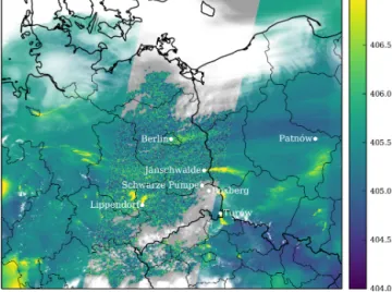
Figure 1. Simulated XCO2field on 23 April 2015 in the
SMART-CARB model domain overlaid with an example of a 250 km wide swath of the planned Sentinel CO2instrument (low-noise scenario).
Missing CO2measurements are shown in gray. Cloud cover is
over-layed in white, with transparency corresponding to total cloud frac-tion.
profiles and at different altitude levels, and which have dif-ferent emission ratios (Brunner et al., 2019). In this study, we therefore carefully consider the vertical and temporal profiles of emissions from different sectors, which makes it possible to test for congruence.
2 Data and methods
2.1 Synthetic satellite observations 2.1.1 Model simulations
The synthetic satellite observations were generated from high-resolution simulations conducted with the COSMO-GHG model. COSMO is a hydrostatic, limited-area model developed by the Consortium for Small-scale Modeling (Bal-dauf et al., 2011), for which an extension has been de-veloped for the simulation of greenhouse gases (COSMO-GHG)(Oney et al., 2015; Liu et al., 2017).
COSMO-GHG was set up to simulate CO2, CO and
NOx concentration fields for nearly the complete year 2015
(1 January–25 December). The model domain extended about 750 km in the east–west and 650 km in the south–north direction. It was centered over the city of Berlin and also cov-ered numerous power plants in Germany and neighboring countries. The spatial resolution was 1.1 km × 1.1 km hori-zontally with 60 vertical levels up to an altitude of 24 km. Figure 1 presents the model domain and marks the location of Berlin and the six largest coal-fired power plants. The de-tailed model setup is described by Brunner et al. (2019).
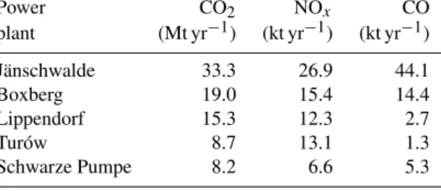
Table 1. Emissions of largest power plants in the model domain according to the TNO/MACC-3 inventory for the year 2011 as used in this study. Power CO2 NOx CO plant (Mt yr−1) (kt yr−1) (kt yr−1) Jänschwalde 33.3 26.9 44.1 Boxberg 19.0 15.4 14.4 Lippendorf 15.3 12.3 2.7 Turów 8.7 13.1 1.3 Schwarze Pumpe 8.2 6.6 5.3
Initial and lateral boundary conditions (ICBCs) for mete-orological variables were provided by the operational Euro-pean COSMO-7 analyses of MeteoSwiss with hourly tem-poral and 7 km horizontal resolution. For the tracers, ICBCs were obtained from the European Centre for Medium-Range Weather Forecasts (ECMWF) through the European Earth observation program Copernicus. CO2 and CO boundary
conditions were taken from a global free-running CO2
sim-ulation with 137 levels and about 15 km horizontal resolu-tion (T1279 spectral resoluresolu-tion, experiment gf39, class rd) (Agustí-Panareda et al., 2014). For NO and NO2, boundary
conditions were taken from ECMWF’s operational global forecasts for aerosol and chemical species with 60 vertical levels and a horizontal resolution of about 60 km (T255 res-olution, experiment 0001, class mc) (Flemming et al., 2015). Anthropogenic emissions were obtained by combining the third version of the TNO/MACC inventory (Kuenen et al., 2014, for version 2), which was generated by the Netherlands Organisation for Applied Scientific Research (TNO) for the Monitoring Atmospheric Composition and Climate – Phase III (MACC-3) project, with a detailed inventory provided by the city of Berlin (AVISO GmbH and IE Leipzig, 2016). The inventories provide point and area sources separately for dif-ferent sectors (e.g., industry, heating and road transport) us-ing Selected Nomenclature for Air Pollution (SNAP) cate-gories. The temporal variability of emissions was accounted for by applying diurnal, weekly and seasonal cycles accord-ing to SNAP categories. Furthermore, emissions were verti-cally distributed using specific vertical profiles for the differ-ent emissions categories and plume rise calculations for the six largest power plants and the major point sources in Berlin (Brunner et al., 2019). Hourly biospheric fluxes of both pho-tosynthesis and respiration were generated with the Vegeta-tion Photosynthesis and RespiraVegeta-tion Model (VPRM) at the resolution of the COSMO model (Mahadevan et al., 2008).
According to the official inventory of the city of Berlin, total annual CO2emissions of Berlin were 16.9 Mt CO2yr−1
(in the reference year 2012 of the inventory). This is about a factor of 2 smaller than in previous studies, e.g., in the LO-GOFLUX project (Chimot et al., 2013; Bacour et al., 2015; Pillai et al., 2016), which relied on unrealistically high
emis-sions as provided by the global EDGAR inventory (version 4.1). Due to the diurnal cycle of emissions, emissions were somewhat larger (about 20.0 Mt CO2yr−1) around the time
of the satellite overpasses (10:00–11:00 UTC). Table 1 sum-marizes the CO2, NOxand CO emissions of the five largest
power plants in the domain.
The simulations included a total of 50 different passively transported tracers representing the three different gases fur-ther divided into different sources, release times or release altitudes. This also included background tracers constrained at the lateral boundaries by the global-scale models and two tracers for biospheric respiration and photosynthesis for CO2. Due to the reactivity of NOx, five different NOxtracers
with e-folding lifetimes of 2, 4, 12, and 24 h and infinity were included, considering that the lifetime of NOxvaries between
about 2 and 24 h (Schaub et al., 2007). The full list of trac-ers is provided in the SMARTCARB final report (Kuhlmann et al., 2019, p. 15f).
In this study we use the following seven tracers that have been computed from the 50 tracers in the simulations.
– X_BER: concentrations from time-varying emissions of Berlin;
– X_PP: concentrations from time-varying emissions from the six largest power plants in the model domain; – X_ANTH: concentrations from other anthropogenic
sources in the domain excluding emissions of Berlin (X_BER) and the six largest power plants (X_PP); – X_BIO: concentrations from local biospheric fluxes,
i.e., respiration and photosynthesis within the domain (only for CO2);
– X_TOT: concentrations from all emissions and bio-spheric fluxes as well as inflow from lateral boundaries; – X_BER_BG: concentrations from emissions, fluxes and lateral boundaries excluding emissions from Berlin (= X_TOT–X_BER); and
– X_PP_BG: concentrations from emissions, fluxes and lateral boundaries excluding emissions from the six ma-jor power plants (= X_TOT–X_PP),
where X is CO2, CO or NO2. NO2concentrations were
cal-culated from NOxconcentrations using an empirical formula
used frequently for representing NO2:NOx ratios
down-stream of emission sources (Düring et al., 2011). For NO2
only the tracers with a lifetime of 4 h were used. Note that only the sum of the emissions from the six power plants was simulated but not the power plants individually, which often complicated the analysis due to overlapping plumes. For the analysis, the three-dimensional model fields were vertically integrated to compute column-averaged dry air mole frac-tions of CO2 (XCO2). Likewise, tropospheric CO and NO2
vertical column densities (VCDs) were generated by consid-ering only the model fields below 10 km altitude.
2.1.2 Satellite instrument scenarios
The CO2M mission is a proposed constellation of satellites flying in a sun-synchronous low-Earth orbit with Equator crossing times around 11:30 local time. Each satellite will carry an imaging spectrometer measuring in the near-infrared (NIR) and in two shortwave infrared spectral bands (SWIR 1 and SWIR 2) for retrieving CO2 as the main payload. The
NIR band is used to retrieve information on the dry air col-umn, on surface pressure, and on aerosols and clouds. The SWIR-1 and SWIR-2 bands contain weak and strong ab-sorption features of CO2and provide additional information
on aerosols and clouds, especially on thin cirrus clouds. A CO2 retrieval using these three bands is described for
ex-ample by O’Dell et al. (2012). CO2M is planned to carry also additional instruments for measuring NO2, aerosols and
clouds. In an earlier phase, also an instrument measuring CO was considered. The preliminary system concept envisages a pixel size of 4 km2and a swath width of 250 km or more.
For the CO2, CO and NO2 satellite observations,
differ-ent instrumdiffer-ent scenarios were prescribed by ESA for this study in terms of orbit, spatial resolution, and spatial and temporal coverage of the CO2M instrument. In addition, the Sentinel-5 instrument on board the Meteorological Opera-tional Satellite – Second Generation A (MetOp-SG-A) was studied as an alternative platform for CO and NO2
measure-ments. Sentinel-5 will be an imaging spectrometer measur-ing, among others, NO2and CO columns with a spatial
res-olution of 7 km× 7 km and a 2650 km swath. MetOp-SG-A will be also on a sun-synchronous orbit but with different Equator crossing times and repeat cycles than the CO2M mission.
In addition to a single satellite, the potential of a constella-tion of multiple CO2M satellites was also studied. The basic assumption for a constellation is that the individual satellites are spaced with equal angular distance in the same orbit with the same orbit parameters, for instance separated by 180, 120 and 90◦ on a full circle in the case of 2, 3 and 4 satellites. The individual satellites can be distinguished by their start-ing longitude at the Equator of the first orbit in the repeat cycle. Here, we analyze constellations between one and six satellites.
For the computation of orbits, we adopted the orbit simula-tor of the Netherlands Institute for Space Research (SRON). Since this simulator makes a few simplifying assumptions, such as circular orbits and tiled ground pixels, satellite and instrument parameters were slightly modified to preserve es-sential parameters. In particular, orbit periods were calcu-lated to match a given cycle duration and length. The pe-riod then determines the altitude and inclination of a circular, sun-synchronous orbit. The altitude of the circular orbits is slightly larger than the typically used mean altitude for el-liptic orbits. Since the altitude affects the size of the ground pixels and the width of the swath, field of view and along-track sampling time were set to match exactly the prescribed
pixel size at subsatellite point as well as the prescribed swath width. As a result, the number of across-track pixels for the simulated Sentinel-5 did not match exactly the number of pixels for the real Sentinel-5 instrument.
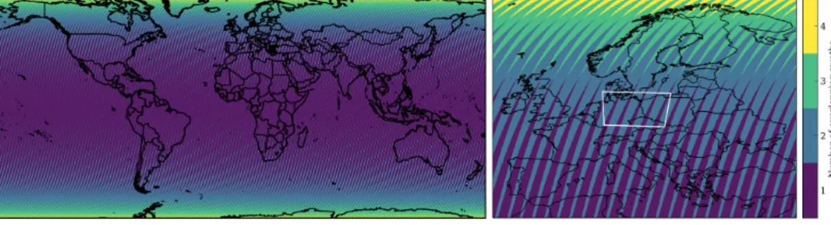
Tables 2 and 3 summarize the orbits and viewing geome-tries of the two satellites. The CO2M satellite is assumed to have a 250 km wide swath and an 11 d repeat cycle. Within the 11 d cycle, the instrument provides nearly global spatial coverage (Fig. 2). For locations in the SMARTCARB model domain, either one or two overpasses occur during the 11 d repeat cycle depending on the Equator starting longitude of the satellite. The wider swath of Sentinel-5 results in near-daily global coverage (not shown).
XCO2, CO and NO2column densities were sampled along
the satellite swath for 1 year using the tracers from the COSMO-GHG simulations. For CO2M, XCO2, CO and NO2
columns were mapped onto the 2 km × 2 km size pixels along the 250 km wide swath.
For Sentinel-5, CO and NO2columns were sampled with
up to 7.5 km × 7.5 km resolution along the 2670 km wide swath of the Sentinel-5 instrument. Due to the wide swath, the pixel sizes grow towards the edge of the swath. In this study, only the spatial overlap between Sentinel-5 and CO2M were of interest because Sentinel-5 was used for detecting the CO2emission plumes inside the swath of CO2M.
2.1.3 Instrument error characteristics
The error characteristics of the CO2, NO2 and CO
instru-ments were specified in collaboration with ESA based on previous studies for CarbonSat (Buchwitz et al., 2013) and on performance requirements for Sentinel-5 (Ingmann et al., 2012). For the instruments on the CO2M satellites, two or three scenarios were included in order to cover a realistic range between more or less demanding instruments. Table 4 summarizes the single sounding precision of the different in-struments.
For XCO2, three different uncertainty scenarios were
con-sidered which relate back to the performance estimates de-rived for the CarbonSat mission concept. CarbonSat was a CO2imaging spectrometer proposed for ESA’s eighth Earth
Explorer mission, with specifications similar to those of the CO2M mission. A detailed error budget for CarbonSat was presented in the CarbonSat report for mission selec-tion (ESA, 2015). In the LOGOFLUX study, error parame-terization formulas (EPFs) for random and systematic errors were developed, which account for errors introduced by solar zenith angle (SZA), surface reflectance in the near-infrared (NIR) and shortwave infrared (SWIR 1), cirrus clouds and aerosol optical depth (Buchwitz et al., 2013).
Here, the same EPFs were adopted but only applied to compute random errors. These were calculated based on SZA and surface reflectance in the NIR and SWIR-1 band. Surface reflectances were taken from the MODIS MCD43A3 product (version 006) at 1 km spatial resolution (Schaaf and Wang,
Table 2. Satellite platforms and their orbit parameters used in this study. Note that some parameters slightly deviate from the real satellites (see text for details).
Parameter CO2M satellite MetOp-SG-A
Orbit type Sun-synchronous Sun-synchronous
Inclination 97.77◦ 98.7◦
Orbits per day 14 + 10/11 14 + 6/29
Cycle duration 11 d 29 d
Cycle length 164 orbits 412 orbits
Altitude 602.24 km 830.16 km
Orbit period 96.58 min 101.36 min
Local time in descending node 11:30 h 09:30 h
(Equator crossing time)
Table 3. Observation geometries for instruments on the CO2M satellite and Sentinel-5 used in this study. Note that some parameters can differ from the real satellites (see text for details).
Parameter CO2M satellite Sentinel-5
Number of across-track pixels 125 208
Swath 250 km 2670 km
Field of view 23.22◦ 107.1◦
Pixel size 2 km× 2 km from 7.5 km× 7.5 km (nadir) to 35 km× 7.5 km (swath edge)
Along-track sampling time 0.286 s 1.13 s
2015). A detailed consideration of cirrus clouds and aerosols and their impact on systematic errors was outside the scope of the study as it would have required the collection and pro-cessing of a large amount of additional data. The possible impact of not considering systematic errors will briefly be discussed in Sect. 4.
The random error calculated with the EPFs for the so-called vegetation-50 scenario (VEG50, i.e., vegetation albedo and SZA of 50◦) is about 1.5 ppm. In the model do-main, mean random errors are slightly smaller at 1.3 ppm. To obtain random errors for the three instrument scenarios with σVEG50 of 0.5, 0.7 and 1.0 ppm, the computed errors were
divided by 3.0, 2.14 and 1.5, respectively.
For NO2 VCDs, the overall uncertainties are due to
(a) measurement noise and spectral fitting affecting the slant column densities; (b) uncertainties related to the separation of the stratospheric and tropospheric column; and (c) uncer-tainties in the auxiliary parameters used for air mass fac-tor (AMF) calculations such as clouds, surface reflectance, a priori profile shapes and aerosols (Boersma et al., 2004). The total uncertainties are dominated by uncertainties from spectral fitting for background pixels and by uncertainties in AMF calculations for polluted pixels, respectively. Typical spectral fitting uncertainties of previous instruments such as the Ozone Monitoring Instrument (OMI) were of the order of 1–2 × 10¹⁵molecules cm−2and AMF uncertainties of the order of 15 %–20 %. These ranges were used to define two different scenarios for a possible CO2M NO2instrument
(Ta-ble 4). For the Sentinel-5 UVNS instrument, we assumed
a relative uncertainty of 20 % and a minimum uncertainty of 1.3 × 10¹⁵molecules cm−2. In the presence of clouds, the reference noise was increased using the empirical formula developed by Wenig et al. (2008). For a cloud fraction of 30 %, random noise is approximately doubled.
For CO VCDs, the total uncertainty depends on the (a) fitting noise; (b) a priori CO and CH4 profiles; and (c)
sur-face reflectance, aerosols and clouds. We assumed a single sounding precision of 4.0 × 10¹⁷molecules cm−2and a rela-tive precision of 10 % and 20 % for both Sentinel-5 and the CO2M mission.
2.1.4 Cloud filtering
Satellite observations require filtering for clouds, which sig-nificantly reduces the number of observations available for plume detection. For the CO2product, we removed all CO2
pixels with cloud fractions larger than 1 % because the CO2
requires rigorous cloud filtering (Taylor et al., 2016). The NO2retrieval can tolerate larger errors and is therefore less
sensitive to clouds. For the NO2 product, we used a cloud
threshold of 30 % as often applied in satellite NO2 studies
(e.g., Boersma et al., 2011). For CO, a cloud threshold of 5 % was used, which is motivated by the cloud threshold used for the MOPITT CO product (Deeter et al., 2017; MOPITT Al-gorithm Development Team, 2017).
Figure 2. Spatial coverage of one CO2M satellite within its 11 d repeat cycle (a) globally and (b) over Europe. The white square marks the COSMO-GHG model domain in which the number of overpasses is either one or two. The exact locations of the stripes are arbitrary and depend on the Equator starting longitude (here: 0◦E) of the satellite.
Table 4. Instrument uncertainty scenarios. VEG50 refers to a reference scene with a surface albedo of a vegetated surface and a solar zenith angle (SZA) of 50◦.
Scenario name Species Satellite(s) Reference noise (σVEG50/σref)
absolute∗ relative∗
CO2low noise CO2 CO2M 0.5 ppm –
CO2medium noise CO2 CO2M 0.7 ppm –
CO2high noise CO2 CO2M 1.0 ppm –
NO2low noise NO2 CO2M 1.0 × 10¹⁵molec. cm−2 15 %
NO2high noise NO2 CO2M 2.0 × 10¹⁵molec. cm−2 20 %
NO2Sentinel-5 NO2 Sentinel-5 1.3 × 10¹⁵molec. cm−2 20 %
CO low noise CO Sentinel-5 and CO2M 4.0 × 10¹⁷molec. cm−2 10 %
CO high noise CO Sentinel-5 and CO2M 4.0 × 10¹⁷molec. cm−2 20 %
∗Whichever is larger.
Previous studies used the MODIS cloud mask product available at 1 km resolution (Ackerman et al., 2017) for masking cloudy CO2 observations (Buchwitz et al., 2013;
Pillai et al., 2016). Since CO and NO2observations can
toler-ate larger cloud fractions, a cloud fraction product would be needed for masking pixels with different thresholds, but the MODIS cloud product is only available at 5 km resolution (Platnick et al., 2017). Therefore, we used total cloud frac-tions computed by COSMO-GHG, i.e., the same model as used for the tracer transport simulations, that are available at model resolution. COSMO-GHG computes total cloud frac-tion from layer cloud fracfrac-tions assuming minimum overlap. The differences between cloud masks derived from COSMO-GHG and MODIS products and their effects on data yield are discussed in Sect. 4.1.
2.2 Plume detection algorithm 2.2.1 Algorithm
We developed a new but simple plume detection algorithm that uses a statistical test to detect signal enhancements which are significant with respect to instrument noise and variability in background levels. The plume is then identified
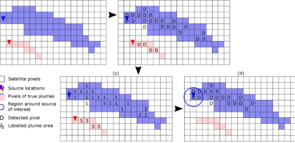
as a coherent structure of significant pixels. The algorithm involves three processing steps as laid out in Fig. 3.
The first step of the plume detection algorithm finds satel-lite pixels with CO2, CO or NO2 values significantly larger
than the background field using a statistical Z test, for which the distribution of the test statistics can be approximated by a normal distribution (e.g., v. Storch and Zwiers, 2003). The Ztest computes a z value given by
z =x − µ
σ , (1)
where x is an observation from a population with mean value µand standard deviation σ . The value x is considered signif-icantly larger than µ when the z value is greater that or equal to a critical value. The critical value is calculated from the inverse cumulative distribution function of the normal dis-tribution for a probability q. The probability that x is not significantly larger than µ is the p value (p = 1 − q).
A key feature of the algorithm is that the trace gas ob-servation of a single pixel is replaced by a spatial average of pixels in a defined neighborhood. This allows identifying weak plumes with signals of individual pixels well below in-strument noise but also bares the risk of diluting the signal at the plume edges. Figure 4 shows examples of neighborhoods
Figure 3. Schematic of the processing steps of the plume detection algorithm. (a) A large (blue) and a small plume (red) with sources marked by arrows are located within the satellite overpass. (b) Pixels detected based on the Z test are marked with “D”. (c) Connected pixels are given a unique number each denoting a different plume. (d) All plumes not connected with the source of interest (blue circle) are rejected.
Figure 4. Examples of neighborhoods with different sizes (ns) used
for calculating the local mean.
with different sizes ns that have been used for testing the
al-gorithm. A large neighborhood results in a stronger smooth-ing and may therefore produce a larger number of false pos-itives, i.e., pixels outside of the plume that are wrongly as-signed to the plume. An ideal neighborhood size balances the need for sensitive plume detection with the requirement of a low fraction of false positives.
Whether a signal enhancement is detectable is primarily determined by the z value (Eq. 1), which can also be in-terpreted as the signal-to-noise ratio (SNR) at a spatially smoothed satellite pixel. Thereby, the signal is the enhance-ment above background due to the plume, and the noise is composed of both instrument noise and spatial variabil-ity in the background. Since the background, i.e., the trace gas field in the absence of the plume, cannot be directly
ob-served, it needs to be estimated either from the observable trace gas field surrounding the plume or from a climatology or a model. Instrument noise and background variability can have both random and systematic components. The random component would reduce with the inverse square root of the number of valid pixels n in the neighborhood, whereas the systematic error would be approximately independent of n. The number of valid pixels n can be smaller than the size of the neighborhood ns when pixels are missing, e.g., due to
clouds or at the boundary of the satellite swath. Therefore, the z value or the SNR can be calculated as follows: SNR =rXobs−Xbg
σ2 rand
n +σsys2
, (2)
where Xobsrepresents the spatially averaged satellite
obser-vations, Xbg is the estimated background value, and σrand
and σsysare the random and systematic errors, respectively.
Equation (2) can be calculated for each satellite pixel and compared with the critical value to determine which Xobs’s
are significantly larger than Xbg.
To compute the SNRs from the satellite image, we com-puted observed values Xobs as the local means of a
neigh-borhood of size ns (Fig. 4). For sake of simplicity, the
back-ground Xbgin this study was estimated from the X_BER_BG
and X_PP_BG model tracers for a 200 km× 200 km square centered on the city of Berlin and a 100 km× 100 km square centered on each power plants. The implications of this as-sumption are discussed in Sect. 4.
For random and systematic errors we assumed that the instrument uncertainty is purely random and that the back-ground variability is purely systematic. For the instrument uncertainty, random errors as listed in Table 4 were used,
which reduce with the number of valid pixels in the local neighborhood n due to the inverse scaling by the number of pixels. The background uncertainty σbg2 was computed from the spatial variance of the background model tracer in a fixed domain surrounding the source as described above. Since it is assumed to be systematic, it does not decrease with the size of the neighborhood.
The result of the Z test is a binary image with “true” val-ues where pixels are significantly enhanced above the back-ground and “false” values where they are not (Fig. 3b). Since the local mean can still be computed for missing center pix-els – using neighboring pixpix-els – missing pixpix-els can also be detected as enhanced above the background.
In the second step, pixels that are enhanced (true) and connected are assumed to belong to the same plume. We label regions of connected pixels using a standard labeling algorithm. Neighboring pixels are identified using a Moore neighborhood, where each pixel has eight potential neigh-bors. Each region is assigned a unique integer value (Fig. 3c). Finally, in the third step, all connected regions that do not intersect with the source region are removed, leaving only re-gions that overlap with the source of the plume (Fig. 3d). For cities, the source region is defined by a circle with a radius of 15 km and for point sources by a circle with a radius of 5 km. The last step may remove regions that are part of the real plume but separated from the source by weak signals or missing values (e.g., the region labeled “2” in Fig. 3c). 2.2.2 Performance evaluation
The plume detection algorithm was applied to the CO2
plumes of Berlin and Jänschwalde. The detectability of CO2
plumes was evaluated for the different instrument scenarios by comparing the detected plume with the “true plume” de-fined by the field of the CO2tracer released by the respective
source (CO2_BER in the case of Berlin, CO2_PP for Jän-schwalde) above a low threshold. For Jänschwalde, the per-formance had to be additionally evaluated by visual inspec-tion due to frequent overlaps with the plumes of other power plants also contained in the CO2_PP tracer.
To evaluate the performance of Sentinel-5 with respect to detecting plumes as observed by CO2M, detected pixels had to be projected onto the pixels of the CO2M instrument. Sentinel-5 pixels were thus only used over the swath of the CO2M satellite rather than over the whole swath of Sentinel-5.
When using NO2or CO for plume detection, the
perfor-mance was assessed by comparing the detected pixels with the true CO2plume rather than the true plume of the
auxil-iary gas. In this way, the degree of congruence between the CO2and auxiliary trace gas plumes was considered as well.
For the evaluation, we computed true positives (TPs), false positives (FPs) and the positive predictive value (PPV = TP/(TP+FP)) (Ting, 2010). A good algorithm should have a much smaller number of FPs than TPs and, therefore, a PPV
close to 1. To remove the impact of different cloud thresh-olds, TPs, FPs and PPVs were only computed for cloud-free pixels using a cloud threshold of 1 % because we are primar-ily interested in valid CO2observations that can be used for
estimating CO2emissions.
3 Results
3.1 Coverage and potential for plume detection
In this section, the potential for plume detection is analyzed based on the simulated tracers emitted by the source of inter-est. These true plumes will be used in the following sections as reference to evaluate the performance of the plume de-tection algorithm. They can be interpreted as the maximum number of plumes detectable by a perfect, noise-free instru-ment.
The frequency with which the CO2 plumes of a given
source can be observed depends on how often a satellite passes over the source, how often the CO2 signal is larger
than the threshold and how often cloud-free conditions dom-inate during the overpass. We define an overpass as an inter-section between the satellite swath and the source region as specified above. The number of overpasses scales with the number of satellites and the swath width of the instrument. The scaling with the number of satellites is not trivial, how-ever, since individual satellites may pass over the source ei-ther once or twice during the 11 d repeat cycle depending on the satellite’s Equator starting longitude (see Fig. 2).
The total number of overpasses per satellite is either 34 or 66 per year, depending on whether the satellite has one or two overpasses per 11 d repeat cycle. Since one out of four satellites has only one overpass per 11 d, the number of over-passes per year roughly scales with a factor 1.75 times the number of satellites times the number of 11 d periods per year (about 33). A constellation of six satellites covers the model domain nearly daily.
To define the extent of a plume in the satellite image, we have to set a signal threshold for the tracer field (XCO2_BER for Berlin) above which a pixel is considered as belonging to the plume. A possible threshold is the value at which the signal would become larger than the variability of the back-ground, i.e., where the signal is larger than the standard devi-ation of the background. Based on the time series of standard deviations of the model background tracer (XCO2_BER_BG for CO2) computed for a 200 km× 200 km square centered
on the city of Berlin (Fig. 7c, f and i), we defined a thresh-old of 0.05 ppm for XCO2, 0.2 × 10¹⁵molec. cm−2for NO2
and 0.06 × 10¹⁷molec. cm−2 for CO approximately corre-sponding to the minimum of the standard deviations. Note that these thresholds are significantly smaller than the noise level of the instruments.
A plume was defined as the collection of pixels for which the signal is larger than the threshold. However, we also
re-Figure 5. Examples of true XCO2plumes of Berlin (XCO2signal > 0.05 ppm) with different cloud cover fractions (cc). The numbers of
XCO2pixels are shown for cloud fractions ≤ 1 %. (a–d) Plumes with increasing cloud fraction; (e) plume close to the edge of the swath;
(f) plume without cloud-free CO2observations connected to Berlin.
quired that Berlin is inside the swath of the instrument to be able to unambiguously assign a plume to the city. Further-more, we removed parts of plumes that reentered the swath after leaving it because it is often not possible to correctly assign these parts to their source.
Since a satellite image can be obscured by clouds, we need to define how many pixels are needed to make up a useful plume. This number depends on the application. For
exam-ple, to estimate emissions of cities, we require that the plume must extend beyond the city limits to contain emissions from the whole city area. The crosswind diameter of Berlin’s CO2
plume is typically about 20 km or 10 satellite pixels, which is roughly the diameter of the part of the city with the high-est emissions. To cover at least the whole city area, we only consider CO2plumes with at least 100 cloud-free CO2
diame-ter is less than 5 pixels near the source. Therefore, 10 pixels were used to define the minimum number for a useful plume in this case. It should be noted that this number of pixels is not necessarily sufficient for estimating the emissions of a source with certain accuracy, which depends, among others, on instrument precision, meteorology and source strength. Nonetheless, detecting the full crosswind diameter is the minimum requirement, for example, for flux-based inversion methods (e.g., Krings et al., 2013; Reuter et al., 2019). The number of detected pixels is a useful measure for comparing the detectability of CO2plumes with CO2, CO and NO2
ob-servations because source strength and meteorology are the same for a given source.
For a signal threshold of 0.05 ppm, Berlin’s CO2 plume
always has more than 100 pixels above the signal thresh-old. However, many plumes are partly or fully covered by clouds significantly reducing the number of useful plumes. Figure 5a–d present examples of CO2plumes under different
cloud conditions with an increasing fraction of cloudy pixels. Figure 5c and d show examples with plumes of only 11 and 20 pixels, which is much smaller than the area of the city. On the other hand, the 100-pixel threshold does not necessarily remove swaths with plumes in broken clouds (e.g., Fig. 5b), for which it will also be challenging to estimate emissions, because adjacent cloudy pixels increase the XCO2
uncer-tainty (Taylor et al., 2016). The number of plumes with at least 100 pixels is also reduced when the source is close to the edge of the swath and winds are pushing the plume out of the view of the satellite (e.g., Fig. 5e). These overpasses occur every 11 d due to the repeat cycle of the satellite. As a result, orbits with plumes near the edge of the swath can have up to 20 % less useful plumes.
Figure 6 presents the number of useful city plumes (> 100 pixels) per month for CO2, NO2and CO for constellations of
one to six satellites. Plumes without cloud-free observations over the source region (e.g., Fig. 5f) were removed because they cannot be detected by the algorithm used in this study. A constellation of six satellites observes only 50 ± 5 CO2
plumes within 1 year despite almost daily overpasses due to the small number of days with low cloud fractions. Ex-cept for February, which was an unusually sunny month in 2015, there is a clear tendency of higher cloud fractions and correspondingly fewer plume observations in winter than in summer. The standard deviations shown in the figures as ver-tical black bars were estimated from the scatter of observable plumes using satellites with different Equator starting longi-tudes. The presence of clouds thus reduces the opportunity for plume detection by a factor as a large as 5 to 6 over the city of Berlin. The number of observable NO2 plumes per
year (108 ± 8) is about twice as large as for CO2, which is
primarily due to the larger cloud threshold of 30 %. For CO the number of observable plumes per year is 58 ± 5. The av-erage number of plumes per satellite and year is thus about 8 (range: 3–13), 9 (4–15) and 17 (7–23) for CO2, CO and NO2,
respectively.
Table 5. The 5th, 50th and 95th percentile of CO2, NO2and CO signals of Berlin as well as Jänschwalde and Lippendorf power sta-tions. Species 5th 50th 95th Berlin CO2(ppm) 0.16 0.33 1.03 NO2(1016molec. cm−2) 0.30 0.63 1.56 CO (1017molec. cm−2) 0.12 0.27 0.96
Jänschwalde power station
CO2(ppm) 1.28 2.69 6.64
NO2(1016molec. cm−2) 2.09 4.30 10.0
CO (1017molec. cm−2) 0.55 1.14 2.88
Lippendorf power station
CO2(ppm) 0.53 1.29 3.73
NO2(1016molec. cm−2) 0.85 2.03 5.37
CO (1017molec. cm−2) 0.03 0.08 0.22
The number of observable plumes varies strongly between the individual satellites of a constellation because the num-ber of cloud-free days per year is quite small and the over-pass days are different for different Equator starting longi-tudes. Since satellites are equally spaced in orbit, changing the number of satellites changes the starting longitudes and overpass days of the satellites. As a consequence, the num-ber of observable plumes per constellation can also fluctuate strongly. According to Fig. 6, for example, a constellation of two satellites seems almost equivalent to a constellation of three, but this result is merely a consequence of the fact that cloud cover was often large during these overpasses and Berlin was at the edge of the swath for the satellite with a starting longitude of 8◦. The result would be different for an-other starting longitude of the first satellite, anan-other city, or another year.
3.2 Signal-to-noise ratios
The key measure that determines the detectability of a CO2
plume is the SNR (Eq. 2), which compares the amplitude of the plume signal to the instrument noise and the variability of the background. SNRs provide a first indication of an in-strument’s suitability for detecting a plume.
Time series of the CO2, NO2and CO plume signals were
computed from the X_BER and X_PP tracers for Berlin and the power stations Jänschwalde and Lippendorf at the overpass time of CO2M, i.e., about 11:00 UTC. The sig-nals were computed as maximum values of the local means within the source region, i.e., a circle with 15 or 5 km radius. Thereby, the local means were computed with a neighbor-hood ns of size 37 for Berlin and 5 for the power stations
(Fig. 4). A large neighborhood reduces the random noise of the measurements and therefore allows detecting smaller
Figure 6. Number of cloud-free plumes of the city of Berlin with at least 100 pixels per month for (a) CO2, (b) NO2and (c) CO. The cloud
threshold is 1 % for CO2, 30 % for NO2and 5 % for CO observations. Error bars are obtained by comparing all available satellites. The
number of expected plumes per satellite is 8, 17 and 9 for the CO2, NO2and CO instrument, respectively.
Table 6. Median signal-to-noise ratios for signals of Berlin, Jän-schwalde and Lippendorf using different uncertainty scenarios. The signals were computed as largest local mean values using a local neighborhood size nsof 37 and 5 for cities and power stations,
re-spectively.
Scenario name Signal-to-noise ratio
Berlin Jänschwalde Lippendorf
CO2low noise 1.4 10.4 4.3 CO2medium noise 1.4 8.0 3.5 CO2high noise 1.2 5.8 2.6 NO2low noise 9.0 14.3 8.8 NO2high noise 8.4 10.8 7.5 CO low/high noise 0.4 0.6 0.0
signals. On the other hand, a large neighborhood will in-clude background values in the computation of the averages at the plume edges and reduce the signal. The sizes used here roughly correspond to the typical diameters of the CO2
plumes from Berlin (about 15 km) and the power stations (about 6 km), respectively, and were also found most suitable for the plume detection algorithm because they maximize TPs without reducing PPVs too much (see also Kuhlmann et al., 2019). The results for Berlin are presented in Fig. 7 for the three trace gases. The figure compares the daily plume signals (left panels) to the daily mean background values (middle) and their spatial variability (right). The 5th, 50th and 95th percentiles of the time series are summarized in Ta-ble 5 for Berlin as well as for the power stations. The sig-nals have a large range due to the variability of emissions (e.g., lower during weekends) and meteorology. The CO2and
Figure 7. Time series of CO2, NO2and CO plume signals (a, d, g); mean backgrounds (b, e, h); and standard deviations of backgrounds (c,
f, i) for Berlin. Signals are the largest local mean values of the X_BER model tracer using a 37-pixel neighborhood. Background means and standard deviations were obtained from the X_BER_BG tracer for a 200 km× 200 km square centered over Berlin. Reference uncertainties (σVEG50/ref) corresponding to the different instrument scenarios are shown as horizontal lines for comparison.
larger than those of Berlin. The CO signal of Lippendorf, on the other hand, is smaller than the signal of Berlin. The power plants produce strong local enhancements easily detectable by the CO2satellite, but the corresponding plumes are much
narrower than those of Berlin.
Figure 7b and c present the spatial means and standard deviations of the background around Berlin. Background XCO2has a strong annual cycle with an amplitude of about
16 ppm. Since the XCO2plume signal of Berlin is typically
only about 0.2 to 1.0 ppm, it is critical to accurately estimate the background XCO2value in Eq. (2). The spatial variability
σbgof the background, on the other hand, is typically only of
the order of a few tenths of a part per million. Despite higher XCO2in winter than in summer, the variability is somewhat
larger in summer due to stronger biospheric activity in com-bination with lower average wind speeds, especially in July and August. Large peaks in the background variability are of-ten caused by plumes from other anthropogenic sources such as the power stations in the southeast of Berlin (Fig. 1).
For NO2, the annual cycle of the background is relatively
constant for our idealized NO2 tracer with a constant
life-time of 4 h (Fig. 7e and f). In reality, the lifelife-time will likely
be longer and the variability correspondingly higher in win-ter. The NO2signal of Berlin is significantly larger than the
background and its variability. Similar to CO2, the CO time
series has a strong annual cycle with an amplitude of about 5 × 10¹⁷molec. cm−2(Fig. 7h and i) requiring again an ac-curate estimation of the background. The standard deviation of the background is about half of the CO signal.
Table 6 summarizes the median of all SNRs of Berlin and the two power stations for the different satellite instru-ment scenarios that have been computed from the time series of highest signals. To understand the numbers, it should be noted that a plume pixel would be detectable when the SNR is larger than 2.3; i.e., z(q) = 2.3 for q = 99 %. For Berlin, the CO2SNRs are below this detection limit for all noise
lev-els while NO2SNRs are above the limit. For the two power
stations, SNRs are above the detection limit both for the CO2
and NO2instrument scenarios, but SNRs for the NO2
instru-ment scenarios are always larger.
Based on the SNRs, the NO2plumes should be well
de-tectable. For Berlin, the detection of the CO2plume with the
CO2instrument will often be challenging due to low SNRs.
Figure 8. Example of plume detection with CO2M’s CO2and NO2instrument and Sentinel-5’s NO2instrument on 21 April 2015. Significant
pixels detected by the algorithm are highlighted as black crosses. The outlines of the true CO2and NO2plumes based on the XBERtracers
are overlaid as solid and dashed lines, respectively. (a) Low-noise CO2instrument. (b) High-noise CO2instrument. (c) High-noise NO2
instrument on the CO2M satellite. (d) NO2instrument on Sentinel-5.
making a CO instrument with the given specifications less suitable for the purpose of plume detection. In the following, we therefore only investigate the potential benefit of auxil-iary NO2observations.
3.3 Plume detection algorithm
The plume detection algorithm was applied to the CO2
plumes of Berlin and Jänschwalde for different instrument scenarios. The probability q was set to 99 % and neighbor-hood sizes of 37 and 5 were selected for Berlin and the power stations, respectively. In the case of Sentinel-5, the corresponding neighborhood sizes were set to 5 and 1 due the larger pixels of this satellite. Based on an analysis of the positive predictive values, these neighborhood sizes were found most suitable for detecting the city and power plant plumes (Kuhlmann et al., 2019). For Berlin, 20 synthetic satellite images were created for each single overpass with different patterns of random noise. The plume detection al-gorithm was subsequently applied to each image, and the re-sults were averaged to obtain more robust rere-sults independent of the selected noise pattern. For Jänschwalde, only one syn-thetic satellite image was created for each overpass because no model tracer was available to compare the results with a true plume.
3.3.1 Examples of detected plumes from Berlin
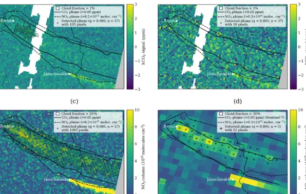
Figure 8 shows the CO2 and NO2 plumes of Berlin on
21 April 2015 observed by CO2M and Sentinel-5 for differ-ent instrumdiffer-ent scenarios. The outlines of the real plumes are overlaid as solid and dashed lines for CO2and NO2,
respec-tively. Since the CO2instruments have a lower cloud
thresh-old, a band of cirrus clouds is obscuring the plume in the CO2observations but not in NO2. Successfully detected
pix-els are shown as black crosses, and the number of detected pixels (median of all 20 noise realizations) are presented in the legend. On average, a CO2instrument detects 116 ± 46,
48±40 and 24±30 pixels with noise scenarios σVEG50of 0.5,
0.7 and 1.0 ppm, respectively (Fig. 8a and b). The number of true positives is slightly smaller, having on average 2 false-positive pixels. Consequently, the PPV is high, ranging be-tween 0.85 and 0.99 for high- and low-noise, respectively.
For the NO2measurement the band of thin cirrus clouds is
not an issue. The NO2instrument can therefore detect a much
larger number of pixels, i.e., 1242 ± 99 and 1203 ± 155 in the case of the low-noise and the high-noise scenarios, respec-tively (Fig. 8c). On average, the fraction of FPs is relarespec-tively large, and the PPV is only 0.80±0.05 and 0.77±0.10 for the low- and high-noise scenarios, respectively. The small PPV is caused by interference with the plume of Jänschwalde, which is just south of the plume of Berlin. For cases where no neigh-boring plumes have been detected falsely with the NO2
in-Figure 9. (a) Example of 27 February 2015 where plume detection with a CO2instrument fails because of pronounced horizontal gradients
in the CO2background field. (c) Example of 2 July 2015 where the plume detection fails due to small CO2signals as a result of high wind
speeds. In both cases, the plume can readily be detected with a high-noise NO2instrument (panels b and d).
strument, the spatial match between CO2 and NO2 plumes
is generally high, suggesting a high degree of spatial overlap between the CO2and NO2plumes.
The Sentinel-5 NO2instrument is also able to detect the
CO2 plume with 879 ± 114 CO2M pixels, but since it is
measured 2 h earlier, the NO2 plume seen by Sentinel-5
(dashed line in Fig. 8d) is slightly shifted with respect to the CO2plume (solid line). As a consequence, the PPVs is low
(0.60 ± 0.04).
Figure 9 presents two examples where the CO2instrument
fails to detect the CO2plume. In Fig. 9a, the CO2field has
a pronounced spatial gradient resulting in a high variance of the background. This gradient is not present in the much-shorter-lived trace gas NO2, making it possible to detect the
plume using an NO2instrument (Fig. 9b). Similar situations
occur in roughly 20 % of cloud-free swaths. Figure 9c and d show a second example where the CO2instrument cannot
de-tect the plume because the signal is very weak due to strong winds. Owing to its better SNR, the NO2instrument is able
to detect the plume also in this situation.
Figure 10 presents two examples comparing the NO2
plume observed by Sentinel-5 to the CO2plume observed 2 h
later by the CO2M satellite. In the first example (panels a and b), Sentinel-5 fails to detect any plume due to clouds, which have largely disappeared by the time of the CO2M overpass. In the second example, both Sentinel-5 and the CO2M satel-lite detect a plume of similar size, but the Sentinel-5 plume is
significantly displaced due to changes in the prevailing winds between the two overpasses.
3.3.2 Number and sizes of detected Berlin plumes To count the number of plumes detectable under the differ-ent instrumdiffer-ent scenarios, we analyze the 50 plumes observed by a constellation of six satellites, which we had classified in Sect. 3.1 as being potentially useful based on the idealized tracer XBERhaving more than 100 pixels above a threshold of
0.05 ppm. Table 7 summarizes the results in terms of number and size of the detected plumes. A plume was only counted as detected when at least 100 CO2pixels were correctly
de-tected (true positives) and when at least 80 % of the dede-tected pixels were true positives (PPV ≥ 0.80). The PPV threshold was found useful for removing plumes interfering with others or plumes shifted due to the earlier overpass time of Sentinel-5.
Table 7 shows that the CO2 instruments detect
signifi-cantly fewer plumes than the NO2 instruments. Depending
on the instrument noise scenario, the CO2 instruments
de-tect plumes with more than 100 pixels with a success rate of only 12 % to 32 %, while for the NO2instruments the
suc-cess rates are 68 % to 70 %. Surprisingly, the NO2instrument
with low noise performs slightly worse than the high-noise instrument. This is an artifact of the algorithm often detect-ing small plumes not related to emissions from Berlin in the case of a low-noise instrument. The Sentinel-5 NO2
instru-Figure 10. Examples of comparing plume detection between the (a, c) CO2M’s and (b, d) Sentinel-5’s NO2instruments. (a, b) Due to a
time lag of 2 h, the scene is cloudy during the Sentinel-5 overpass but not during the CO2M overpass (3 December 2015). (c, d) The plume position clearly changed between the two overpasses (17 June 2015).
ment detects 20 % of the plumes, thus only half the success rate of the NO2instrument on the CO2M satellite. The main
reason for this low success rate is the spatial mismatch of the plumes due to the 2 h difference in overpass times.
Figure 11 shows the number of plumes per month with at least 100 detected pixels for different constellations be-tween one and six satellites for the CO2low-noise and the
NO2 high-noise scenario. The number of plume detections
per month is small and therefore highly sensitive to the spe-cific orbit configuration. For example, two satellites seem to detect more plumes than three, but this result is caused by an unfavorable orbit for observing Berlin for the constellation with three satellites and unfavorable cloud cover as already discussed earlier. The standard deviation was estimated from the number of detectable plumes using satellites with differ-ent starting longitudes (i.e., east–west displacemdiffer-ents of all orbits). The figure shows that the number of observed plumes generally increases with the number of satellites as expected, but statistical noise can mask the increase from one constella-tion to the next. The figure confirms the much lower success rates of the CO2instruments as compared to the NO2
instru-ments as expected from the computed signal-to-noise ratios. 3.3.3 Detection of plumes from power stations
There are six major power plants in the model domain: Jän-schwalde, Boxberg, Schwarze Pumpe, Lippendorf, Turów and P ˛atnów. Because no model tracer was defined for
in-dividual power plants but instead only for the sum of all of them, the true plume of an individual power plant is not known. Therefore, we applied a visual inspection to identify those plume detections which erroneously included neigh-boring plumes. Furthermore, we limit the analysis to Jän-schwalde.
As an example, Fig. 12 shows the successful detection of the CO2plume of Jänschwalde on 2 November 2015 by
dif-ferent instruments. Since CO2emissions of Jänschwalde are
high with 33.3 Mt CO2yr−1, the XCO2signal is very strong
and can be detected well even with a high-noise instrument (σVEG50=1.0 ppm). With low noise (σVEG50=0.5 ppm) the
weaker plumes of Schwarze Pumpe and Boxberg are visi-ble as well. The NO2 instrument detects the four plumes
in the region well. On this day also the Sentinel-5 NO2
in-strument successfully detects the plume of Jänschwalde and other point sources. Figure 13 presents a second, more chal-lenging example for 17 February 2015. The CO2instrument
successfully detects the plume with 0.5 ppm uncertainty, but with 1.0 ppm uncertainty, the number of detected pixels is likely too small to be useful for emission estimation. The reason for the low number of detected pixels in this case is the strong horizontal gradient in the CO2background. The
NO2 instrument detects the plume, but because the NO2
plume of Jänschwalde overlaps with neighboring plumes, these plumes are erroneously assigned to Jänschwalde as well. At the coarser resolution of Sentinel-5 the plumes of the
Table 7. Number of CO2plumes from Berlin and the 5th, 50th and 95th percentiles of the number of detected CO2pixels (TP if PPV ≥ 0.8 and cloud fraction < 1 %) for a constellation of six CO2M satellites or one Sentinel-5 satellite. The maximum number of detectable plumes would be 50, corresponding to all potentially useful plumes with at least 100 CO2pixels with values of the tracer XBERabove a threshold
of 0.05 ppm.
Instrument scenario Plumes with ≥ 100 CO2pixels Plume size at percentile
number percentage (%) 5th 50th 95th CO2low noise 16 ± 1 32 ± 3 0 5 323 CO2medium noise 10 ± 1 20 ± 3 0 3 261 CO2high noise 6 ± 1 12 ± 2 0 7 181 NO2low noise 34 ± 1 68 ± 2 52 294 600 NO2high noise 35 ± 2 70 ± 3 50 279 527 NO2Sentinel-5 10 ± 2 20 ± 3 0 140 396
Figure 11. Number of detected plumes with at least 100 pixels (TP ≥ 100 and PPV ≥ 0.80) for one to six satellites with the (a) CO2low-noise
and (b) NO2high-noise scenario. Error bars were estimated from all available satellites with different Equator starting longitudes.
individual power plants can hardly be separated and, more-over, the time difference of 2 h results in a plume location that is shifted with respect to the plume seen by the CO2M satellite.
Table 8 summarizes the results of the plume detection for Jänschwalde under the different instrument scenarios. It shows the number of detected plumes with at least 10 pixels and, in addition, the number of plumes with at least 10 valid CO2 pixels (cloud cover < 1 %). Note that, in the case of
the much narrower plumes from power plants, fewer pixels are required to form a useful plume. We classified detections that include large parts of the background as failed but still counted detections that include neighboring plumes as suc-cessful (e.g., Fig. 13c) because they sucsuc-cessfully identified
the location of the plume. Since the classification is not al-ways unambiguous, we assigned an uncertainty of about ±5 plumes at most.
In the year 2015, the number of detectable plumes with more than 10 pixels for a constellation of six satellites was between 40 and 45 for a CO2instrument with σVEG50of 0.5,
0.7 and 1.0 ppm. At the same time, the NO2instrument
de-tected about 90 plumes for the low- and high-noise scenario. When only plumes with more than 10 cloud-free CO2
obser-vations were considered, the number was reduced to about 70 plumes. For a smaller number of satellites, the number of de-tectable plumes would be correspondingly smaller. The NO2
instrument detects more plumes because of its lower sensi-tivity to clouds, which makes it possible to trace the plume
Table 8. Number of plumes detected for Jänschwalde with six satellites. The number of plumes are provided for plumes with at least 10 detected CO2or NO2pixels and in addition with at least 10 CO2pixels (cloud cover < 1 %). In both cases, plumes were included where
neighboring plumes were detected in addition to Jänschwalde, i.e., detection with a large number of false positives (e.g., Fig. 13c). These plumes are also shown separately. The classification uncertainty is about ±5 plumes. The neighborhood size was set to ns=5.
Instrument Number of plumes with
scenario ≥10 detected pixels ≥10 CO2pixels large number of false positives
CO2low noise 44 42 7
CO2medium noise 42 40 6
CO2high noise 41 40 4
NO2low noise 90 68 38
NO2high noise 91 68 34
Figure 12. Example of plume detection for the Jänschwalde power plant on 2 November 2015 using (a, b) the CO2instrument with σVEG50
of 0.5 and 1.0 ppm, (c) the NO2instrument with the high-noise scenario and (d) the NO2instrument on Sentinel-5.
to the source even for partly cloudy scenes. On the other hand, the NO2instrument often detects overlapping plumes
(e.g., Boxberg and Schwarze Pumpe) because the instrument is much more sensitive to small signals further away from the origin than the CO2 instrument. The mean plume size
was about 100 pixels for the low-noise CO2instrument. The
plumes detected with the high-noise CO2 instrument were
about half the size. The NO2instruments detected a similar
number of CO2pixels to the low-noise CO2instrument, but
when all detected pixels are counted the number of pixels doubles.
4 Discussion
4.1 Comparison with previous studies
In this study we investigated whether and how frequently the CO2plume of Berlin and power stations can be detected by
different constellations of satellites using either CO2
obser-vations alone or in combination with obserobser-vations of the co-emitted trace gases CO and NO2. To address the question,
high-resolution CO2, CO and NO2fields were simulated with
the COSMO-GHG model for the year 2015 and used to gen-erate synthetic XCO2, CO and NO2satellite observations for
Figure 13. Example of plume detection for Jänschwalde power plant on 17 February 2015 using (a, b) the CO2instrument with σVEG50of
0.5 and 1.0 ppm, (c) the NO2instrument with the high-noise scenario and (d) the NO2instrument on Sentinel-5.
OSSEs studies were conducted by Pillai et al. (2016) and Broquet et al. (2018) for Berlin and Paris, respectively, as part of the LOGOFLUX study (Bacour et al., 2015). How-ever, their simulations did not include NO2 and CO fields.
A fundamental difference of our study compared to previous studies is the realistic, i.e., not as a random noise, account for transport model errors in the present study, where the loca-tion of the plume is not taken from the model but detected in the satellite image using either CO2or NO2observations.
For this reason, the focus of this paper is on the detectabil-ity of the plume, while Pillai et al. (2016) and Broquet et al. (2018) focused on the inversion, which we will describe in a follow-up publication.
Pillai et al. (2016) simulated CO2 fields with the
WRF-GHG model with 10 km× 10 km spatial resolution for the year 2008. The resolution was relatively low compared to the 1.1 km× 1.1 km resolution used in our study. They used CO2
emissions from the EDGAR inventory (version 4.1), which are more than twice as high as the emissions reported in the inventory of the city of Berlin as mentioned earlier. A consequence of the unrealistic high emissions is higher CO2
signals (0.80–1.35 ppm) for Berlin than in our study (0.16– 1.03 ppm; see Table 5). Note that the signal strength also
de-pends on the spatial resolution, but our XCO2 signals were
computed for a local mean (ns=37, i.e., 148 km2 spatial
resolution) that is comparable to the model resolution used by Pillai et al. (2016). For Paris, Broquet et al. (2018) con-ducted simulations with the CHIMERE atmospheric trans-port model with 2 km spatial resolution. CO2emissions for
the greater urban area were 40–50 Mt CO2yr−1, which
re-sulted in a XCO2 signal of ∼ 1 ppm, quite consistent with
the plume signals reported here.
For Berlin, we estimated that 3 to 13 potentially useful CO2 plumes (defined as plumes with at least 100
cloud-free pixels above a threshold of 0.05 ppm) would be observ-able, but not necessarily detectobserv-able, during 1 year by a single CO2M satellite with a 250 km wide swath. Pillai et al. (2016) identified 41 potentially useful orbits for estimating emis-sions with a 500 km wide swath. Although a direct compari-son of these two numbers is difficult because of the different swath widths and the different definitions of “usefulness”, we can still conclude that our study identified significantly fewer plumes than Pillai et al. (2016) even after halving their number to account for their wider swath.
Clouds have a strong impact on the number of cloud-free observations. A major difference between Pillai et al.