HAL Id: hal-02491802
https://hal.archives-ouvertes.fr/hal-02491802
Submitted on 26 Feb 2020
HAL is a multi-disciplinary open access
archive for the deposit and dissemination of
sci-entific research documents, whether they are
pub-lished or not. The documents may come from
teaching and research institutions in France or
abroad, or from public or private research centers.
L’archive ouverte pluridisciplinaire HAL, est
destinée au dépôt et à la diffusion de documents
scientifiques de niveau recherche, publiés ou non,
émanant des établissements d’enseignement et de
recherche français ou étrangers, des laboratoires
publics ou privés.
On the interpretation of linear relationships between
seafloor subsidence rate and the height of the ridge
Caroline Dumoulin, M.-P Doin, L. Fleitout
To cite this version:
Caroline Dumoulin, M.-P Doin, L. Fleitout. On the interpretation of linear relationships between
seafloor subsidence rate and the height of the ridge. Geophysical Journal International, Oxford
Uni-versity Press (OUP), 2001, �10.1046/j.1365-246X.2001.00490.x�. �hal-02491802�
On the interpretation of linear relationships between seafloor
subsidence rate and the height of the ridge
C. Dumoulin,* M.-P. Doin and L. Fleitout
Laboratoire de Ge´ologie, Ecole Normale Supe´rieure, 24 Rue Lhomond, 75231 Paris Cedex 05, France. E-mail: [email protected]
Accepted 2001 April 12. Received 2001 February 2; in original form 1999 December 23
S U M M A R Y
Several studies have found that the ‘subsidence rate’ of the oceanic lithosphere measured along flow lines is a linear function of the height of the ridge. This might have very important implications concerning our understanding of the cooling of the lithosphere. Here we study the relationship between the subsidence rate and the height of the ridge in the South Atlantic and East Indian Oceans. From the regression slopes of this relationship, it has been inferred that lithosphere created at shallower ridges subsides faster and to deeper levels than that generated at deeper ridges. We show however, that the topo-graphy at young ages for various seafloor segments stays positively correlated with the topography at older ages. Synthetic data sets are obtained by adding random synthetic signals with the same spectrum as the residual topography to the average depth versus age relationship. They are also characterized by the same linear relationship between ‘subsidence rates’ and the height of the ridge. This relationship is therefore not proof that lithosphere formed at shallow ridges cools faster than lithosphere formed at deeper ridges. Random signals linked with crustal thickness variations, hotspot bulges and perhaps large wavelength ‘dynamical topography’ would also yield such a relationship. Key words: heat flow, mid-ocean ridges, oceanic lithosphere, seafloor spreading, thermal subsidence.
1 I N T R O D U C T I O N
Several studies have shown a clear linear relationship between the subsidence rate and the height of the ridge (hereinafter referred to as zero-age depth) both deduced from the regression between seafloor depth and the square root of age. Such a relation-ship was obtained by Hayes (1988), Hayes & Kane (1994), Kane & Hayes (1994a,b) with subsidence rates computed along swaths parallel to flow lines. Kane & Hayes (1994b) deduced from this relationship that seafloor segments with a ridge shallower than average acquire depths greater than average after a crossover age of about 10 Ma. Hayes & Kane (1994) found (in their separate studies over three different oceans) large differences of average zero-age depths from one ocean to another. Marty & Cazenave (1989) computed the subsidence rates, not along swaths, but over 32 broad areas covering almost the whole oceanic floor. They also report a good correlation between subsidence rates and zero-age depths that yields a crossover age of about 60 Ma. The discrepancy between this crossover age and that of Kane & Hayes (1994b) can be explained by the existence of large offsets of average zero-age
depth between the various oceans. The study of Perrot et al. (1998) concerns the Pacific ridge and emphasizes variations with time of zero-age depth and subsidence rate.
Kane & Hayes (1994b) argue that ridge segmentation is a long-lived structure. The relationship between zero-age depth and subsidence rate seems to indicate large temperature variations along the ridge which may persist along the same segment for at least 30 or 40 Ma and influence the topography. Stationary elongated convective cells below the young oceanic lithosphere and/or the presence of hotspots in the vicinity of the ridge may explain these long-lasting characteristics of the ridge segmenta-tion (Kane & Hayes 1994a). More generally, knowing whether lithosphere formed above a hot mantle subsides faster or more slowly than average might be the key issue for understanding the mode of cooling of the oceanic lithosphere.
However, we must note that the slope of depth versus square root of age is not necessarily a real subsidence rate. Real sub-sidence rates can only be known in the rare areas where palaeo-bathymetry data are available. For example, the Rio-Grande Rise at 30uS, 35uW was above sea level when it formed at the ridge some 84 Ma ago Barker (1983). However, the ridge on the same flow line is now at a depth of about 3000 m. In this case, as for any segment close to an oceanic plateau, the depth of the ridge varies with time and slopes of bathymetry versus
* Now at: Universite´ Joseph Fourier, Maison de Ge´osciences, LGIT, BP. 53, 38041 Grenoble Cedez 9, France.
square root of age do not provide real subsidence rates but reflect variations in the thickness of passively advected crust. In order to use the same terminology as the previous studies, we will name the slope of topography versus square root of age ‘subsidence rate’, the quotes reminding the reader that this might be an improper term. Processes influencing the ocean floor bathymetry, but not directly linked to seafloor spreading and lithospheric cooling, possibly induce a relationship between ‘subsidence rate’ and zero-age depth.
In this paper, we study two areas: the South Atlantic and the East Indian Oceans. We determine the relationship between zero-age depths versus ‘subsidence rates’ along flow lines using a method similar to that proposed by Kane & Hayes (1994b). The correlation of the topography at a given age with the topography near the ridge is also discussed. Finally, random noise maps are added to the average cooling signal to provide synthetic data sets. The relationship between zero-age depths and ‘subsidence rates’ obtained on such data sets is then compared with the observed data.
2 D A T A A N A L Y S I S M E T H O D
The ‘subsidence rates’ and zero-age depths are computed from oceanic bathymetry, sediment thickness and crustal age. The bathymetry derives from the 2k by 2k gridded database of Sandwell (Smith & Sandwell 1997; Smith & Sandwell 1994) that uses ship soundings where they are available, and predicted bathymetric values based on Geosat/ERS-1 gravity anomalies in data gaps. In this database a smooth transition from measured to predicted bathymetric values is insured by the mapping technique. Nevertheless, only points close to ships tracks will be used in this study. The sediment thickness database has been compiled by the National Geophysical Data Center (NGDC), from three main sources: previously published isopach maps, ocean drilling results, and seismic reflection profiles (Divins 1991). The data are gridded with a grid spacing of 5k by 5k. The digital crustal age grid has been built with a 6k interval, using a self-consistent set of global isochrons and associated plate reconstruction poles (Mueller et al. 1997). This study is focussed on the South Atlantic Ocean between 4uS and 49uS and between 325uE and 360uE, and on the East Indian Ocean between 30uS and 65uS and between 73uE and 130uE.
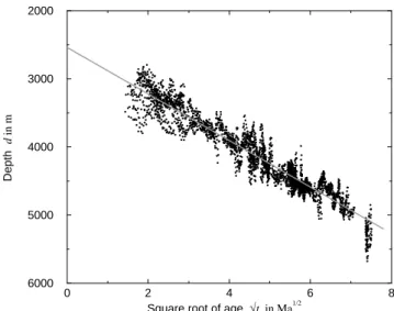
We create and analyse profiles with the same methodology as Kane & Hayes (1994b). Profiles consist of couplesðd,pffiffitÞ, all located in the same corridor, where d is the bathymetry corrected from sediment loading (assuming isostasy as in Colin & Fleitout 1990), and t is the crustal age. Points located further than 4 arc min from a ship track are suppressed. In the South Atlantic Ocean, profiles extend to 60 Ma (see Fig. 1), whereas they spread only to 40 Ma in the East Indian Ocean.
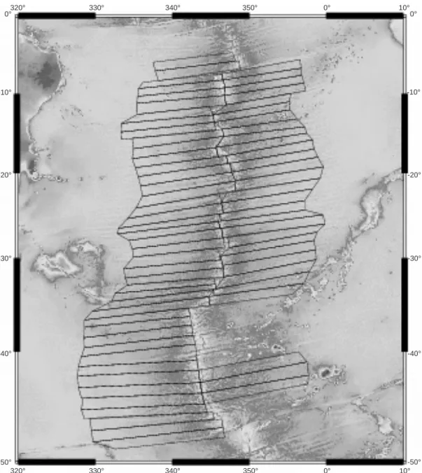
As in Calcagno & Cazenave (1994), Kane & Hayes (1994a,b), Hayes & Kane (1994) and Perrot et al. (1998), corridors are defined along flow lines, i.e., parallel to transform faults. The seafloor in such corridors has been generated at the same ridge segment. Therefore, if ridge segmentation is responsible for long lived differences in crustal thickness, asthenosphere temperature, and basalts density or chemistry (see Calcagno & Cazenave 1993; Klein & Langmuir 1989, 1987; Lecroart et al. 1997), profiles along flow lines should reflect uniform physical characteristics. Profiles do not overlap (Fig. 2 shows flow line locations for the South Atlantic Ocean, Fig. 3 shows locations for the East Indian Ocean)
The following relation, reflecting the cooling of the litho-sphere (Turcotte & Oxburgh 1967), is adjusted to every profile of more than 100 points:
d~d0zSr|
ffiffi t p
, (1)
where d0is the zero-age depth and Srthe ‘subsidence rate’. The bootstrap technique (Kane & Hayes 1994b) is used to calculate Sr, d0 and their estimated uncertainties sSr and sd0. These uncertainties depend on the number of points in the profile studied. They are not absolute estimates of errors, as the data points (d, t) are not geographically independent. However, these uncertainties quantify the relative quality of the linear regressions (1) for different profiles. Therefore they will be used in the next step of the analysis to weight the obtained estimates of Srand d0.
The relations between zero-age depth and ‘subsidence rate’ computed for all profiles of a given flank are then calculated by a linear regression weighted by their relatives uncertainties sSr and sd0(Press et al. 1994, p. 660):
d0~DzM|Sr: (2)
The slope M [in m (m Max1/2)x1] is called the ‘interswath correlation’ by Kane & Hayes (1994b). Let us note that regression (2) is not performed here using a least square method which would be appropriate for noise only on d0. The absolute values of M found here are then somewhat larger than in some previous studies (Kane & Hayes 1994b). Errors on M cannot be estimated as neighbouring flow lines present Srand d0values that are not geographically independent. The regression has been performed on profiles all having exactly the same mean square root of agepffiffit. Indeed, the mean square root of age can be taken as a reference value when studying a statistical effect. The coupleðd,pffiffitÞ is the barycentre of a set of points in a given corridor. In consequence, the regression line (1) goes through this point: d0~d{Sr| ffiffi t p : (3)
If all profiles have the same average bathymetry d, independent of Sr, then the slope M of the linear regression between d0and Srover an ocean will be equal to {
ffiffi t p
(compare (3) with (2)). In
0 2 4 6 8
Square root of age √t in Ma1/2
6000 5000 4000 3000 2000 D e p th d in m
Figure 1. Example of a bathymetric profile along flow line in the South Atlantic Ocean.
692 C. Dumoulin, M.-P. Doin and L. Fleitout
the following, the relationship (M) between ‘subsidence rates’ Srand zero-age depths d0 will be systematically studied as a function of the mean square root of age (pffiffit) for both the South Atlantic and East Indian Oceans.
3 P R O P E R T I E S O F T H E ‘ S U B S I D E N C E R A T E ’ V E R S U S R I D G E H E I G H T
R E L A T I O N S H I P
The amplitude of ‘subsidence rate’ variations are about 400 m Max1/2 for the East Indian Ocean and about 300 m Max1/2 for the South Atlantic Ocean. The amplitude of zero-age depth variations are about 2000 m for both oceans. For example, Fig. 4 shows the linear relationship (2) for the South Atlantic Ocean withpffiffit~3:5 Ma1/2.
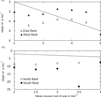
For both oceans, the absolute slope M of the linear regression (2) is, at young ages, often larger than the mean square root of age and is independent ofpffiffit(see Fig. 5). This slope is larger for
the East Indian Ocean than for the South Atlantic Ocean. Note that a least-square regression of d0 as a function of Sr with errors only applied to d0 (as in Kane & Hayes 1994b) yields absolute values of M that are smaller than those shown on Fig. 5 but still larger thanpffiffit.
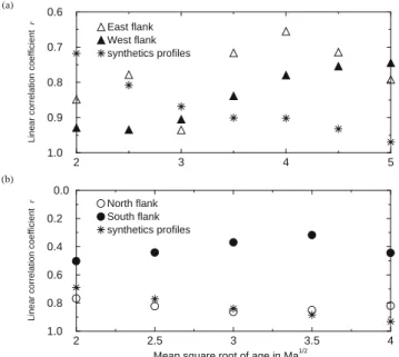
Fig. 6 shows that the linear correlation coefficient r between Srand d0is rather good and ranges fromx0.7 to x1 for both flanks of the South Atlantic Ocean and for the northern flank of the East Indian Ocean, but that it is poor, betweenx0.3 andx0.7, for the southern flank of the East Indian Ocean. The latter low r values result in large uncertainties on M, that could explain why larger slopes M are obtained by the linear regression for this flank (Fig. 5b).
Kane & Hayes (1994b) conclude from the observed anti-correlation between d0and Srthat shallower ridges subside to greater depths than deeper ridges. Therefore depth versus age profiles should cross each other at about M2, called the ‘crossover age’ (i.e., at about 10 Ma for the South Atlantic Ocean). If this
320° 330° 340° 350° 0° 0° -10° -20° -30° -40° -50° 10° 0° 350° 340° 330° 320° -50° -40° -30° -20° -10° 0° 10°
Figure 2. Corridors along flow lines in the South Atlantic Ocean. On the southern part of the east flank, we did not study corridors going through the Walvis Ridge and seamounts, because of their large associated bathymetry anomalies.
is true, it implies an anticorrelation between the bathymetry at the ridge and that of older oceans. Fig. 7 shows the depth averaged over 5 Myr wide intervals (from 0–5 Ma to 50–55 Ma) as a function of the corridor number, for the western flank of the South Atlantic Ocean. One notices that there is no evidence for this anticorrelation. This is confirmed in Fig. 8, where the regression slopes between the mean bathymetry for 0–5 Ma (bold curve in Fig. 7) and the mean bathymetry for the other age intervals (solid or long-dashed curves in Fig. 7) are shown to be always positive, whatever the ocean and flank studied. In other words, shallower than average ridge segments correspond to shallower than average tectonic corridors, at least until 35–50 Ma. This surprising observation is the most direct way to prove that the linear relationship between Srand d0does not
imply an anticorrelation between the topographies at young and old ages. It can be explained by the existence of very large wavelengths in the bathymetric maps that are superimposed on the depth–age distribution responsible for the anticorrelation
60° 70° 80° 90° 100° 110° 120° -30° -40° -50° -60° -30° -40° -50° -60° 130° 60° 70° 80° 90° 100° 110° 120° 130°
Figure 3. Corridors along flow lines in the East Indian Ocean.
550 450 350 250 150 50
Subsidence rate Sr in m.Ma1/2 3500 3000 2500 2000 1500 Z er o a g e de p th d0 in m East flank West flank
Figure 4. Linear relationships between ‘subsidence rate’ Srand
zero-age depth d0 for the South Atlantic Ocean and for
ffiffi t p
=3.5 Ma1/2.
Linear regressions yield M=x3.80 Ma1/2, D=x3694 m, and r=0.72
for the East flank (long-dashed light line), and M=x2.73 Ma1/2,
D=x3404 m, and r=0.84 for the West flank (long-dashed bold line).
2 2.5 3 3.5
5
Mean square root of age in Ma1/2 25 20 15 10 5 0 s lo p e M in Ma 1/ 2 North flank South flank 2 3 4 6 5 4 3 2 s lo p e M in Ma 1/ 2 East flank West flank (a) (b) 4
Figure 5. Variations of the slope M of the linear regression with the mean square root of age, (a) for the South Atlantic Ocean and (b) for the East Indian Ocean. Solid lines represent the supposed statistical effect: M=xpffiffit.
694 C. Dumoulin, M.-P. Doin and L. Fleitout
between d0 and Sr. Ridge height variations for the southern flank of the Indian Ocean are perfectly correlated with the bathymetry variations at an older age. Note that this flank is also the one that presents the worst Sr versus d0 regression coefficients and the larger discrepancy between M and {pffiffit.
4 C O M P A R I S O N O F R E G R E S S I O N S C O M P U T E D F R O M R E A L O R
S Y N T H E T I C B A T H Y M E T R Y M A P S
Here, we check whether the relationship obtained between ‘subsidence rates’ and zero-age depths can be due to random noise. This noise consists of bathymetric anomalies that are not related to oceanic accretion, lithospheric cooling, and to their variations in amplitude along the ridge axis. An upper bound on the noise amplitude and spectrum can be computed by removing the average cooling signal from the bathymetric data. Therefore, we first correct the bathymetry for the average cool-ing effect, 2691z328pffiffit{0:046t2(Colin & Fleitout 1990). We
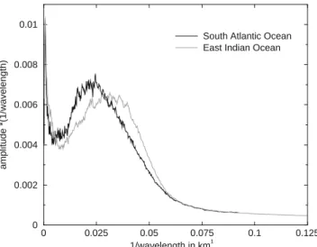
then reduce the influence of pronounced bathymetric anomalies by applying a cut-off on hotspots tracks, and finally, we com-pute the wavelength spectrum of reduced bathymetric maps (see Fig. 9). These maps cover areas similar to the oceanic regions studied previously.
We then build artificial noise maps with a wavelength spectrum similar to that of the reduced bathymetric data.
(i) The real and imaginary parts (in the Fourier domain) of the noise are filled with random numbers having a Gaussian distribution centred on 0 and of half-width 0.2.
(ii) The values in these grids are adjusted to the amplitude, for equal wavenumbers, of the reduced bathymetry spectrum. (iii) We then perform an inverse Fourier transform to get a noise map on a grid similar to that of the oceans studied.
(iv) Finally, the average cooling effect has been added back to the noise maps in order to compare the results obtained by the analysis of synthetic bathymetry maps to the results obtained with the data.
2 2.5 3 3.5 4
Mean square root of age in Ma1/2
1.0 0.8 0.6 0.4 0.2 0.0 L inear c orre lation c oeffi c ient r North flank South flank synthetics profiles 2 3 4 5 1.0 0.9 0.8 0.7 0.6 L inear c orre lation c oeffi c ient r East flank West flank synthetics profiles (a) (b)
Figure 6. Variations of the linear correlation coefficient r with the mean square root of age, (a) for the South Atlantic Ocean and (b) for the East Indian Ocean. Stars represent the mean linear correlation coefficient for 20 studies on noise maps built on reduced bathymetry of oceans. r is calculated as follows:
r¼ P i ðSriÿ SrÞ|ðd0iÿ d0Þ ffiffiffiffiffiffiffiffiffiffiffiffiffiffiffiffiffiffiffiffiffiffiffiffiffiffiffiffi P i ðSriÿ SrÞ2 r | ffiffiffiffiffiffiffiffiffiffiffiffiffiffiffiffiffiffiffiffiffiffiffiffiffiffiffiffi P i ðd0iÿ d0Þ2 r : 10 0 10 20 30 40 Corridor number 6000 5000 4000 3000 2000 1000 Bathy me tr y, in m d0 05 1015 2025 3035 4045 5055 5,21 S0 29,6 S0 47,6 S0
Figure 7. Bathymetry average over 5 Ma wide segments for each corridor as a function of the profile number, for the West flank of the South Atlantic Ocean. Bold solid curve is the mean bathymetry near the ridge (0–5 Ma). The (alternately) solid and long-dashed curves represent from top to bottom the bathymetry averaged over intervals varying from 5–10 Ma to 50–55 Ma with an increment of 5 Ma (age slices are given for each long-dashed curve). The dotted curve represents zero-age depths. The latitude at the middle of the ridge segment is given for three different corridors.
0 2 4 6 8
Square root of age in Ma1/2
0.5 0 0.5 1 1.5 R egre ss ion sl o p e
South Atlantic, east flank South Atlantic, west flank East Indian, north flank East flank, south flank Example of synthetic profile
Figure 8. Slope of linear regressions between the seafloor depth average for ages between 0 and 5 Ma and the seafloor depth average for ages between i and (i+5) Ma, where i increases every 5 Ma from 0 to 35 Ma for the East Indian Ocean and from 0 to 50 Ma for the South Atlantic Ocean. The slope of the linear regression is plotted as a function of the square root of agepffiffiffiffiffiffiffiffiffiffiffiffiffiffiiþ 2:5Ma1/2. The example shown here by stars has been calculated from a synthetic bathymetry map built on the South Atlantic Ocean. Standart errors on the slope are represented with error bars (dashed for South Atlantic Ocean, solid for East Indian Ocean and gray for the example on a synthetic noise).
Note that the largest wavelength in the noise map corresponds to the length of the area of study.
20 different noise maps have been computed for each ocean. On each synthetic map, the ’ridge’ is arbitrarily taken at the middle of the grid, i.e. at even latitude for synthetic maps based on the East Indian Ocean and at even longitude for synthetic maps based on the South Atlantic Ocean. Synthetic profiles are defined perpendicularly to the ‘ridge’. They present even widths of 1.4u (0.8u, respectively) and are artificially extended to 40 Ma (60 Ma, respectively) for synthetic maps based on the reduced bathymetry of the East Indian Ocean (South Atlantic Ocean, respectively). An example of a synthetic profile is shown in Fig. 10, and should be compared to Fig. 1. The amplitudes of the seafloor depth deviations from the average cooling effect are of the same magnitude in synthetic and in real cases.
Exactly the same treatment as used for real bathymetric data is then applied to the synthetic profiles. The linear relation-ships between Srand d0present similar characteristics to those obtained using real bathymetry (cf Fig. 11). Indeed, the variation
ranges of Srand d0are only slightly greater when using syn-thetic maps than when using data. The slope M of the linear regression between d0and Srhas been computed for both ‘flanks’ of 20 different synthetic maps. On Fig. 12 the distribution of M is plotted for various values of pffiffit. Fig. 12(a) should be compared with the South Atlantic Ocean results (Fig. 5a) and Fig. 12(b) with the East Indian Ocean results (Fig. 12b). Both figures show that M is often different frompffiffitand independent of the mean square root of age of the profiles. We can conclude that for random noises the probability of M being independent of pffiffit is high. However, note that the results of the analysis on the synthetic maps do not explain all the properties of the relationship between Srand d0in the Indian Ocean. First, M is aroundx10 Ma1/2
, whereas for the synthetic profiles (Fig. 12b) the highest probability gives M=x4 Ma1/2
. Second, we obtain clearly lower values of r for the southern flank of the Indian Ocean than those expected from a random noise (see stars on Fig. 6). 0 0.025 0.05 0.075 0.1 0.125 1/wavelength in km1 0 0.002 0.004 0.006 0.008 0.01 am p lit ud e *( 1 /wavelength )
South Atlantic Ocean East Indian Ocean
Figure 9. Wavelength spectrum of reduced bathymetry maps for the South Atlantic and the East Indian Oceans.
0 2 4 6 8
’Mean square root of age’ √t in Ma1/2
6000 5000 4000 3000 2000 ’D e p th ’ d in m
Figure 10. Example of a profile extracted from a synthetic data set whose noise is based on the reduced bathymetry of the South Atlantic Ocean. This figure should be compared to Fig. 1.
800 600
400 200
0
Subsidence rate Sr in m.Ma1/ 2
4000 3000 2000 1000 Z er o a g e de p th d0 in m ’East flank’ ’West flank’
Figure 11. Example of a linear relationship between Sr and d0 for
profiles extracted from a synthetic data set and with a mean square root of age of 3.5 Ma1/2. The random noise in the synthetic data set is based
on the South Atlantic Ocean reduced bathymetry. This figure should be compared to Fig. 5(a). Linear regressions yield M=x3.06 Ma1/2,
D=x3691 m, and r=x0.92 for the ‘East flank’ (light dashed line), and M=x4.63 Ma1/2, D=x4120 m, and r=x0.99 for the ‘West
flank’ (bold dashed line).
2 3 4 7 5 3 1 Slope M in Ma 1/ 2 (a) 2 3 4
Mean square root of age in Ma1/2 7 5 3 1 Slope M in Ma 1/ 2 (b) 5
Figure 12. Histograms of the slope M distribution for the 20 different noises based on (a) the South Atlantic Ocean and (b) the East Indian Ocean, plotted as a function of mean square root of age (pffiffit) of profiles. The dashed line represents the line M¼ ÿpffiffit.
696 C. Dumoulin, M.-P. Doin and L. Fleitout
One example of the correlation between variations in ridge depths and of ocean depths at older ages is displayed by stars on Fig. 8. As for the other synthetic maps, the correlation drops to about zero for ages larger than 17 Myr. This reflects random perturbations of the synthetic bathymetry along flow lines. To obtain an autocorrelation between ridges height and bathymetry at older ages (as for real data), we need to add a wavelength with a preferred orientation (with highs and lows striking along the flow line direction) to the random noise syn-thetic maps. We built a map of such synsyn-thetic noise. Its ridge height variations are, of course, strongly autocorrelated with depth variations at older ages, but it also has poor correlation coefficients r between Srand d0, and the absolute slopes M are large and strongly depart frompffiffit. For the southern flank of the Indian Ocean, shallow ridges correspond to shallow tectonic corridors. We conclude that this excellent autocorrelation destroys the quality of the Sr versus d0 relationship (low r, Fig. 6b) and is responsible for the very large absolute values of M (Fig. 5b) with respect to what would be expected from random bathymetry fluctuations. The same remarks, but to a lesser extent, could also apply to the eastern flank of the Atlantic Ocean.
Other tests have been performed on synthetic noise maps having a spectrum amplitude that increases with wavenumber, remains constant, and decreases with wavenumber. In the first case, the regression coefficient r is excellent and the slope M varies with {pffiffit. As the large wavelength content of the noise spectrum increases, r decreases, and M becomes more independent of {pffiffit. Therefore the fact that M differs from and does not vary with {pffiffitin the Atlantic and Indian Ocean can be explained by the importance of large wavelength content in residual bathymetric maps.
5 C O N C L U S I O N S
In this study, we show that similar linear relationships between ‘subsidence rates’ and zero-age depths are observed on syn-thetic maps, where a noise map is superimposed to the average cooling signal, and on real maps. In both cases, the slope of the linear relationship, M, can be very different from the assumed statistical effect, {pffiffit. This discrepancy is explained by the very large wavelength content in the residual bathymetric maps. The regression line through any random signal has a slope showing a very well defined anticorrelation with the vertical coordinate of its origin. However, the seafloor bathymetry at old ages seems well correlated with the ridge height variations, a feature that is not reproduced by synthetic noise maps. Adding such an autocorrelation signal to the synthetic noise maps reduces the quality of the regression between ‘subsidence rates’ and zero-age depths and increases the discrepancy between M and {pffiffit. The presence of a very large wavelength bathymetric anomaly on the South flank of the Indian Ocean can in the same way explain the properties of the ‘subsidence rates’ versus zero-age depths relationship on this flank. It seems therefore very difficult to separate the ‘ridge height’ versus ’subsidence rate’ signal linked to the cooling of the lithosphere from that coming from trivial ‘statistical’ relationships. Furthermore, in contrast to the conclusions of Kane & Hayes (1994b), a lithosphere originating at a shallow ridge appears to remain shallower than average.
Several processes not related to the cooling of the lithosphere affect the topography and could therefore generate a statistical ‘subsidence rate’ versus zero-age depth relationship. Deep mantle masses and plate motions produce very large wave-length dynamic topography that are expected to be moderately correlated to seafloor age and of at most a few hundred metres in amplitude (Cadek & Fleitout 1999; Colin & Fleitout 1990). Besides, topographic variations of the order of one kilometre are associated with hotspots swells. These are more or less randomly distributed at the surface of the Earth. Moreover, changes in the thickness of the crust and of the depleted mantle layer produce significant variations of topography. Klein & Langmuir (1987) and Lecroart et al. (1997) have shown using geochemical data and seismic data that these changes in the thickness of the crustal and depleted layers were indeed the main cause of variations in the height of the ridge. These fluctuations could yield random variations of ‘subsidence rate’ but have no reason to induce a topography at old ages systematically deeper when the ridge is shallow.
The autocorrelation between ridge heights and seafloor depths at old ages can be explained if there are long-lasting temperature anomalies below the ridge (for example, when hotspots and/or stationary secondary convection cells are fixed with respect to the ridge geometry) inducing long-lasting topographic highs and lows along flow lines associated with crustal thickness variations.
The influence of lithospheric cooling processes on the ridge height versus ‘subsidence rate’ relationship depends on the model we consider.
(i) The simplest idea is to consider that the subsidence rate varies linearly with mantle temperature as expected from the half-space model or the plate model. However, as emphasized by Kane & Hayes (1994a), the expected variations in mantle temperatures are too small for accounting for the huge variations in observed ‘subsidence rates’.
(ii) In contrast with the plate model, the Chablis model yields subsidence rates depending mostly on the heat transfer at the base of the lithosphere (Doin & Fleitout 1996). Therefore in this model an elevated mantle temperature (shallow ridge) induces a large heat transfer and hence a small subsidence rate. (iii) A third hypothesis is that the thickness of the con-ductive plate (in the plate model) is fixed by the depleted layer below the crust. Indeed, a stiff depleted layer can stabilize the lithosphere (Doin et al. 1997). Then, a higher temperature at the ridge yields a thicker depleted layer and a deeper bathy-metry at old ages; even if the initial subsidence rate remains the same, it persists until larger seafloor ages for thick plates corresponding to shallow ridges.
The above statistical analysis shows that, at present, the observed ridge height versus ‘subsidence rate’ relationship cannot help to discriminate between the various lithospheric cooling models. A more sophisticated statistical analysis would be needed to know whether a lithosphere formed above a hot mantle subsides faster or more slowly than the normal mantle.
A C K N O W L E D G M E N T S
The authors thank H. Schmeling, G. Marquart, and an anonymous reviewer for their useful comments. This work was supported by the program CNRS-INSU-IT.
R E F E R E N C E S
Barker, P.F., 1983. Tectonic evolution and subsidence history of the Rio Grande Rise, Init. Repts. DSDP, LXXII, 953–976.
Cadek, O. & Fleitout, L., 1999. A global geoid model with imposed plate velocities and partial layering, J. geophys. Res., 104, 29 055–29 975. Calcagno, P. & Cazenave, A., 1993. Present and past regional ridge segmentation: evidence in geoid data, Geophys. Res. Lett., 20, 1895–1898.
Calcagno, P. & Cazenave, A., 1994. Subsidence of the seafloor in the Atlantic and Pacific Oceans: regional and large-scale variations, Earth planet. Sci. Lett., 126, 473–492.
Colin, P. & Fleitout, L., 1990. Topography of the ocean floor: thermal evolution of the lithosphere and interaction of deep mantle hetero-geneities with the lithosphere, Geophys. Res. Lett., 17, 1961–1964. Divins, D.L., 1991. Total Sediment Thickness of the World’s Oceans &
Marginal Seas, NOAA National Geophys. Data Center, Boulder, CO. Doin, M.P. & Fleitout, L., 1996. Thermal evolution of the oceanic lithosphere: an alternative view, Earth planet. Sci. Lett., 142, 121–136.
Doin, M.-P., Fleitout, L., Christensen, U., 1997. Mantle convection and stability of depleted and undepleted continental lithosphere, J. geophys. Res., 102, 2771–2787.
Hayes, D.E., 1988. Age-depth relationships and depth anomalies in the Southeast Indian Ocean and South Atlantic Ocean, J. geophys. Res., 93, 2937–2954.
Hayes, D.E. & Kane, K.A., 1994. Long-lived mid-ocean ridge seg-mentation of the Pacific-Antartic ridge and the Southeast Indian ridge, J. geophys. Res., 99, 19 679–19 692.
Kane, K.A. & Hayes, D.E., 1994a. Long-lived mid-ocean ridge seg-mentation: constraints on models, J. geophys. Res., 99, 19 693–19 706.
Kane, K.A. & Hayes, D.E., 1994b. A new relationship between sub-sidence rate and zero-age depth, J. geophys. Res., 99, 21 759–21 777. Klein, E.M. & Langmuir, C.H., 1987. Global correlations of ocean ridge basalt chemistry with axial depth and crustal thickness, J. geophys. Res., 92, 8089–8115.
Klein, E.M. & Langmuir, C.H., 1989. Local versus global variations in ocean ridge basalt composition: A reply, J. geophys. Res., 94, 4241–4252.
Lecroart, P., Albare`de, F. & Cazenave, A., 1997. Correlations of Mid-Ocean Ridge basalt chemistry with the Geoid, Earth planet. Sci. Lett., 153, 37–55.
Marty, J.C. & Cazenave, A., 1989. Regional variations in subsidence rate of oceanic plates: a global analysis, Earth planet. Sci. Lett., 94, 301–315.
Mueller, R.D., Roest, W.R., Royer, J.Y., Gahagan, L.M., Sclater, J.G., 1997. Digital isochrons of the world’s ocean floor, J. geophys. Res., 102, 3211–3214.
Perrot, K., Francheteau, J., Maia, M., Tisseau, C., 1998. Spatial and temporal variations of subsidence of the East Pacific Rise (0-23S), Earth planet. Sci. Lett., 160, 593–607.
Press, W.H., Teukolsky, S.A., Vetterling, W.T., Flannery, B., 1994. Numerical recipies in Fortran, 2 edn, Cambridge University Press, Cambridge.
Smith, W.H.F. & Sandwell, D.T., 1994. Bathymetric prediction from dense altimetry and sparse shipboard bathymetry, J. geophys. Res., 99, 21 803–21 824.
Smith, W.H.F. & Sandwell, D.T., 1997. Global sea floor topography from satellite altimetry and ship depth soudings, Science, 102, 10 039–10 054.
Turcotte, D.L. & Oxburgh, E.R., 1967. Finite amplitude convective cells and continental drifts, J. Fluid Mech., 28, 29–42.
698 C. Dumoulin, M.-P. Doin and L. Fleitout