Modeling ozone and carbon monoxide redistribution by shallow convection over the Amazonian rain forest

HAL Id: hal-02025355

https://hal.uca.fr/hal-02025355

Submitted on 6 Feb 2021

HAL is a multi-disciplinary open access

archive for the deposit and dissemination of

sci-entific research documents, whether they are

pub-lished or not. The documents may come from

teaching and research institutions in France or

abroad, or from public or private research centers.

L’archive ouverte pluridisciplinaire HAL, est

destinée au dépôt et à la diffusion de documents

scientifiques de niveau recherche, publiés ou non,

émanant des établissements d’enseignement et de

recherche français ou étrangers, des laboratoires

publics ou privés.

Modeling ozone and carbon monoxide redistribution by

shallow convection over the Amazonian rain forest

J. Edy, S. Cautenet, P. Brémaud

To cite this version:

J. Edy, S. Cautenet, P. Brémaud. Modeling ozone and carbon monoxide redistribution by shallow

convection over the Amazonian rain forest. Journal of Geophysical Research: Atmospheres, American

Geophysical Union, 1996, 101 (D22), pp.28671-28681. �hal-02025355�

ß

Modeling ozone and carbon monoxide redistribution by shallow

convection

over the Amazonian

rain forest

J. Edy and S. Cautenet

Laboratoire de Meteorologie Physique, Universite Blaise Pascal, CNRS, Aubiere, France

P. Brmaud

Laboratoire de Physique Atmosphere, Universire de l'ile de la Reunion, St. Denis, France

Abstract. During a "locally occurring

system"

(LOS) in Amazonian forest characterized

by an active mixing layer from surface to 1000 m capped by a fossil mixed layer between 1000 and 1500 m, the vertical mixing effects of a shallow cumulus are examined. The explicit redistribution of CO and 03 has been studied with a two-dimensional convective cloud model coupled with a chemical model including gas and aqueous phases, for a shallow convective situation taken from the GTE/ABLE 2B campaign. The chemistry describes the main oxidation chains of CH 4 and CO in presence of low NOx concentration in a remote troposphere. Model results compare favorably with observations obtained after development of the shallow convection. The analysis of results explains how a growing and decaying cloud field allows exchanges between a mixing layer, a fossil mixed layer and the free troposphere. An inert tracer study has shown that the layer lying between surface to 500 m is transported up to 2000 m. Even small clouds are responsible for the transport and the transformation of chemical species. Sensitivity tests are

performed to evaluate the relative importance of dynamical, microphysical and chemical processes. The cumulus venting is the main process which modifies the trace species redistribution. The 0 3 and CO amounts which are transported by a fair-weather cumulus through the boundary layer and free troposphere in the wet season, over a tropical rain

forest,

are respectively

1.2 x 1023

molecules

km

-2 h -1 and 7.7 x 1023

molecules

km -2

h -•. In tropical

regions,

over

rain forest,

even

with low NOx concentration,

several

cumulus exist every day and the vertical fluxes of some chemical species (like 03) cannot be neglected.

1. Introduction

The impact of clouds on the transfer of trace species from boundary layer to the free troposphere is very important in both cases of shallow and deep convection. In tropospheric chemistry, three processes are modified by the presence of clouds: the transport of chemical species, the photochemistry and the aqueous phase chemistry. Several authors have dem-

onstrated that convective clouds constitute a mechanism for

intense vertical transport, through observations [Ching et al., 1986; Gidel, 1983; Garstang et al., 1988; Lyons et al., 1986] or through inert tracers modeling [Lafore and Moncrieff, 1989; Pickering et al., 1990; Chaumerliac et al., 1989; Renard et al., 1994]. Clouds have not only the potential to transport chemical species from the mixed layer to the overlying free troposphere but also clouds can transform and modify many chemical spe- cies by aqueous phase chemistry occurring in droplets [Cha- meides and Davies, 1982; Jacob, 1986].

In evaluating regional CO and 0 3 budgets, Thompson et al. [1994] show the important effect of convective transport over the Central United States. They estimate that both shallow cumulus and synoptic scale weather systems are as efficient as deep convection, but they point out that relative CO and 0 3 fluxes due to shallow convection and synoptic scale weather

Copyright 1996 by the American Geophysical Union. Paper number 96JD01867.

0148-0227/96/96JD-01867509.00

systems are poorly known. Observations of O_• distribution inside and outside the clouds apparently lead to different 03 evolution, depending on the type of clouds (small cumulus or stratiform clouds) [Preiss et al., 1994].

Detailed simulations of clouds and photochemistry in con- vective situations have highlighted a great degree of variability in dynamical structure and in trace gases redistribution from one event to another one [Scala et al., 1990; Pickering et al., 1990, 1991; ChatfieM and Delany, 1990].

All these studies have been achieved using off-line models, without any aqueous chemistry. They show the dominant role of transport during deep convection. More recently, a convec- tion cloud model, explicitly coupled with a gas/aqueous chem- ical model [Gr•goire et al., 1994] exhibits the role of microphys- ical processes on the redistribution of chemical species among the aqueous and gas phases. With a similar chemistry model, LelieveM and Crutzen [1991] show the role of clouds on 03 redistribution. They have estimated that if the air is spending 3 at 4 hours inside the clouds in NOx poor region, net ozone destruction rates are enhanced by factors ranging from 1.7 to 3.7 [Graedel and Crutzen, 1993].

The preceding works, however, have no experimental sup- port. In this paper, we intend to compare model results with experimental data. Using a cloud model coupled with a gas/ aqueous chemical model, we examine the role of the aqueous chemistry in shallow convection when vertical velocity and liquid water content are lower than in deep convection.

e('K) looo (m) a) h e i h t o eœ('K) 295 310 335 i 380 14 q (g/kg) i i i i i

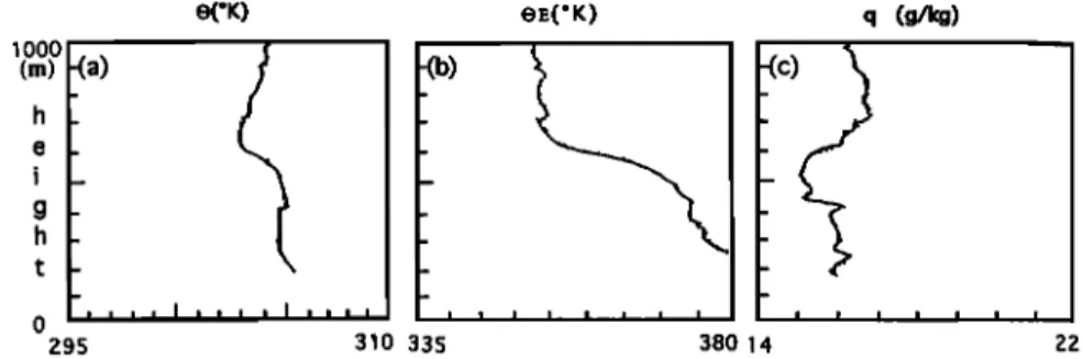
Figure 1. Tethered balloon profile at 1200 local standard time (LST) on May 4, 1987, at Ducke. (a) Potential temperature, (b) equivalent potential temperature, and (c) specific humidity (from M. Garstang, personal communication, 1995).

The equatorial forests are an important source of organic acids [Talbot et al., 1990] which can lead to ozone destruction by aqueous chemistry processes. During the GTE/ABLE2B campaign in 1987 (Journal of Geophysical Research, 95, 16,721- 17,050, 1990) in Amazonia, an observation of a fair cumulus cloud was performed and vertical profiles of CO and O3 were measured by an instrumented aircraft, the NASA Electra be- fore and after a succession of convective cells developments. Ritter et al. [1990] have examined the influence of such a cloud field on species distributions in the subcloud layer. We use these data to validate our coupled model, and we examine the relative importance of different processes on chemical species distribution due to the presence of small cumulus. Although O3 is a low soluble species, we want to investigate whether the competition between the three governing processes (transport, photochemistry, aqueous chemistry) is important in a case of

shallow convection where the vertical velocities are weak but

where the liquid water content is not negligible, as in equato- rial forest regions.

After a short presentation of experimental data and of the model, we show the comparison between the simulated and observed profiles. Then, sensitivity tests are performed to as- sess the relative importance of dynamical, microphysical and chemical processes which are competing inside a shallow cu-

mulus.

The case under study represents a local system which in- cludes a fossil mixed layer lying between 1000 and 1500 m over a tropical rain forest during the wet season. A cumulus pene- trates into this layer and destroys it. We examine and evaluate the exchanges between the fossil mixed layer and the mixing

layer.

2. Experimental Data

The synoptic situation for May 4, 1987, over the central

Amazon Basin is consistent with fair-weather conditions, asso-

ciated with shallow convection and small cumulus. This is typ- ically a so-called "locally occurring system" (LOS), character- ized by surface divergence until midafternoon, followed by

weak convergence associated with the growing convection

[Greco et al., 1990].

The description of the meteorological situation is the fol- lowing: the 700 hPa streamlines pattern shows a convergence line which lies north-south (NS) along 55øW from just north of the equator to about 7.5øS with equatorial vortex centred near 54øW and 0øS. Low level flow (5 m above canopy) at 1120 LST

exhibits divergent easterlies across network. A high-pressure center is observed over Tabatinga; another weak high-pressure center lies on the coast at 10øS, with a ridge between. A NS cloud line is revealed by satellite infrared data at 0900 LST along 55øW with center to the north of Belem coast, whereas a clear area extends to the west of Manaus-Tabatinga. Manaus eastward shows the edge of a system along 55øW. At the 250- hPa level, flow shows an anticyclone centred near 1.5øS, 52.3øW (Amazon mouth) supporting the north/south convergence line. This situation is not likely to undergo rapid changes.

The detailed evolution of the weather from aircraft data is described below:

1. Cloud amounts mainly of fair weather cumulus (CU-1 at 1118 LST) and later (1312 LST) cumulus congestus (CU-2) were present throughout the flight but decreasing in amount from 7/8 sky cover to 4/8 sky cover.

2. Cloud base is ranging between 875 m at 1138 LST and 1100 m at 1501 LST; cloud top locates between 1625 m at 1136

LST and 1719 m at 1501 LST.

3. Inversion base ranging between 1250 m at 1134 LST and

1812 m at 1320 LST.

4. Light showers appeared over the area of operations and were probably present soon after 1300 LST and clearly visible

from the aircraft between 1440 and 1457 LST.

On the same day (May 4, 1987), a fair-weather cumulus was studied by Ritter et al. [1990] between 1130 LST and 1440 LST. There were no upper level clouds except isolated patches of cirrus far away. By 1130 LST the convective cloud field became

more isolated, and cloud cover decreased to 5/8. By 1440 LST

the convective cloud development was over.

2.2. Thermodynamical Analyses

This undisturbed day is characterized by a typical mixed layer found above the Amazonian rain forest. The tethered

balloon observations and comments which follow have been

given by M. Garstang (personal communication, 1995). The tethered balloon observations show a vertical potential tem- perature profile (Figure la) with adiabatic conditions from surface to 1000 m at 1200 LST. Also, the vertical equivalent potential temperature (Figure lb) and the specific humidity (Figure lc) profiles look well mixed, although the latter de- creases slowly with height over the first 1000 m.

By 1137 LST (Figure 2) a moist adiabatic layer is observed between 1000 and 1200 m, a sharp inversion from 1200 to 1300 m and a secondary moist adiabatic layer from 1300 to 1600 m. The layer from 1000 to 1800 m roughly agrees with the

75O 800 850 900 95O lOOO 1050

On Skew-T/i og-P Diagram

Moisture Temperature

2000

1500

lOOO

500

Figure 2. Temperature and moisture profiles obtained dur- ing the vertical sounding taken at 1137 LST [from Ritter et al., 1990].

By 1300 LST, gradients are evident in the vertical potential temperature profile (Figure 3a), in the vertical equivalent po- tential temperature profile (Figure 3b) and in the specific hu- midity profile (Figure 3c). Downdrafts penetrate the mixing layer and a mixing zone exists between the cloud layer and the mixed layer. This is obviously due to the action of precipitation convection. The depth of the mixed layer has now descended to about 500 m suggesting downward mixing from the cloud layer penetrating to this level.

By 1344 LST we observe (Figure 4) that the inversion zone (from 1400 to 1500 m) has weakened and a moist adiabatic

layer extents from 1500 to 1700 m.

2.3. Chemical Data

Figures 5 and 6 represent the CO and 0 3 profiles for the two soundings: 1137 and 1344 LST. They both show that O3 con- centration increases with height, while CO concentration de- creases. Negative correlation between CO and 0 3 in the lower troposphere reflects a sink for O3 at the surface and a source for CO [Harris et al., 1990]. With low (8 ppt) NO concentration

(Table 1) there is no O3 production; photochemistry repre-

sents a weak sink for O 3 [Jacob and Wofsy, 1990; Scala et al.,

1990].

For O3 we observe (Figure 5) two mixed layers with constant values: the first below 1000 m where 03 concentration is 12 ppbv and the second above 1400 m where 0 3 concentration is

20 ppbv, which is about twice the values observed near the ground. Between these two mixed layers exists a strong positive

gradient of 10 ppbv km -• from 1000 to 1200 m and of 30 ppbv

km- • from 1200 to 1400 m associated

to the inversion

layer.

The lower value of 12 ppbv observed below 1000 m is explained by deposition during nighttime and in the morning without exchange with the above layers (as the fossil one for instance).

The CO profile (Figure 5) slowly decreases with height be- low 1000 m. This profile has a different pattern below 1000 m and above 1000 m, and we observe, as for 03 profile, that during nighttime and the morning there is no exchange with the above layers. Moreover, above 1000 m a sharp negative CO

gradient exists from 1000 to 1200 m with a minimum of 105

ppbv at 1200 m. Then, above 1400 m we see strong alternate

positive or negative gradients.

The initial profiles (Figure 5) are consistent with a well established mixed layer (from surface to 800 m) and a shallow cloud convective layer between approximately 900 and 1700 m. Enhanced 03 content in and above this cloud layer (1000 to above 2000 m) and regions of relatively high CO content (such as the layer near 1500 m) are associated with the previous day's fossil mixed layer and with layer structures due to inversions in the subsidence synoptic scale environment. Frequently, fossil mixed layers over Amazonian rain forest [Martin et al., 1988] are observed, generally during undisturbed days. In this case, the boundary layer at 1137 LST, is characterized by an active

On 6kew-T/Log-P Diagram .... Moisture Temperature

700

," ,"L'" ,"

,"

%,

,, .,'

.,'

.,'

,,

,

'

,37'

Figure 4. Temperature and moisture profiles obtained dur- ing the vertical sounding taken at 1344 LST [from Ritter et al.,

1990]. iooo h i g h t o •95 O(øK) e •. (" K) q (g/kg)

-(a)

-

Figure 3. Tethered balloon profile at 1300 LST on May 4, 1987, at Ducke. (a) Potential temperature, (b)

equivalent potential temperature, and (c) specific humidity (from M. Garstang, personal communication, 1995).

Ozone, ppbv 0 10 20 30 40 50 ... , .... , .... , ... 750 •co -- 0 3

2000

-

/

800

1500

•

850

soo

Figure 5. 0 3 (dashed !ine) and CO (solid line) species mix-

ing ratio profiles obtained during the initial sounding of Figure 1 [from Ritter et al., 1990].

mixing layer from surface to 1000 m capped by a fossil mixed

layer between 1000 and 1500 m, mixed but not mixing.

In Figure 6, after the development of shallow convection, we observe a smoothing in the 03 vertical profile and the gradients are much more homogeneous than in Figure 5. The CO profile (Figure 6) is less mixed than 03 and has a similar shape than the water vapor profile. This pattern may be explained because the CO source is the ground surface. Figure 6 profiles exhibit the clear signature of a precipitating cumulus which mixes both layers (fossil and underlying mixing layer).

In the case of 0 3 , higher cloud layer values of 03 have been mixed downward into the mixed layer and lower mixed layer

values elevated into the cloud layer. In the case of CO, high

values prevail near surface (below 750 m), but a general de- crease with cloud/precipitation mixing has occurred above 750 m. The stratified and layered nature is evident.

3. Description of the Chemical Transport

The chemical model [Gr•goire et al., 1994] is coupled with a convection model. It monitors 12 chemical species in gaseous and aqueous phases as introduced by Lelieveld and Crutzen [1990,

3000 2500 2000 1500 1000 5OO Ozone, ppbv 20 30 o lO 40 5o -, , , ß i .... i •....•, , , i .... • ....

'"• •"

---co

700

./

'

Figure 6. 03 (dashed line) and CO (solid line) species mix- ing ratio profiles obtained during the sounding of Figure 4 [from Ritter et al., 1990].

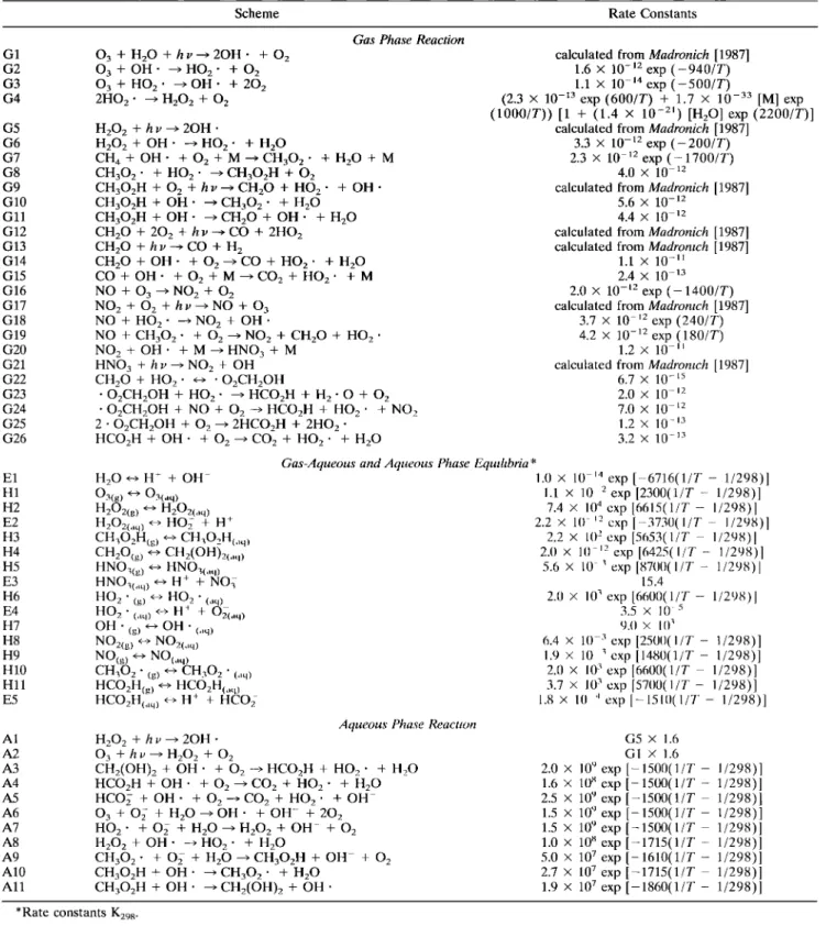
1991]. It describes the main oxidation chains of CH 4 and CO in presence of NOx in a remote troposphere. Its kinetic scheme presented in Table 2 contains 26 reactions and equilibrium in the gas phase, 16 gas/aqueous phase equilibrium, and 11 aqueous phase reactions. The rate of reaction G4 has been modified, following Stockwell [1994], to account for its dependency on water vapor and temperature, a feature which was neglected by Le- lieveld and Crutzen [1991] and also by Grdgoire et al. [1994]. The photolysis rates calculated according to Madronich [1987] for local conditions are assumed constant with time, but may vary

with the altitude and the location of the cloud layers. The

complete chemical scheme then leads to a set of two primary

equations which express the rate of concentration changes

between gas and aqueous phases, including mass transfer con- siderations. Those equations are solved by the Hesstvedt [1978] solver with a time step of 0.5 s when cloud is present, and a time step of 15 s otherwise. For more details, the reader is referred to Grdgoire et al. [1994].

The cloud model is a two-dimensional (x, z), time- dependent, Eulerian scheme [Cautenet and Lefeivre, 1994]. It is

nonhydrostatic and anelastic. Three bulk water categories are

considered here: vapor, cloud water and rain water. These hydrometeors interact through a variety of physical processes (e.g., condensation, evaporation, autoconversion, coalescence, accretion, and collection). The basic assumptions in the micro- physical processes used are (1) a monodisperse, time invariant cloud droplet population in which the total number of droplets is fixed; (2) droplet coalescence (autoconversion) computed using the Kessler [1969] formulation with a threshold; and (3) rain distribution following Marshall and Palmer's [1948] distri- bution. Surface energy fluxes are prescribed which allow trig- gering and maintenance of cloud cycles. The horizontal spatial grid resolution is 200 m. The vertical spatial grid resolution is

100 m in order to be able to describe a fine structure of thermo-

dynamic profile commonly observed within shallow cloud layers.

The overall dimension of the modeled domain is 3.2 km in the

vertical and 6.4 km in the horizontal. The time step of inte- gration is 15 s. The duration of the simulation is 2 hours.

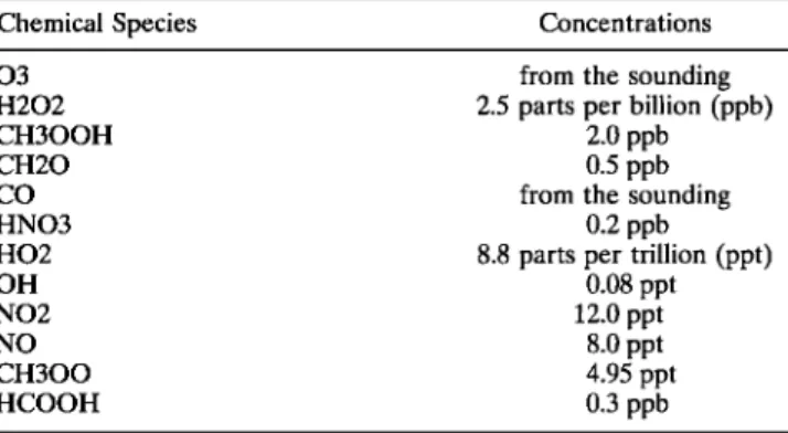
We initialize the model with the atmospheric sounding (Fig- ure 2) along with 03 and CO profiles (Figure 5) at 1137 LST. For the other species, we take vertically homogeneous profiles in ppb (Table 1), according to Jacob and Wofsy [1990] and Singh et al. [1990]. The pH is held constant and equal to 5, a typical value of precipitation acidity during ABLE 2B cam- paign [Jacob and Wofsy, 1990].

The ground budget is prescribed as follows [Fitzjarrald et al., 1990]: the net radiative flux at the beginning of the simulation

Table 1. Initial Values of Chemical Species in the Gas

Phase That Are Used to Initialize the Chemical Module

Chemical Species Concentrations

03 from the sounding

H202 2.5 parts per billion (ppb)

CH3OOH 2.0 ppb

CH20 0.5 ppb

CO from the sounding

HNO3 0.2 ppb

HO2 8.8 parts per trillion (ppt)

OH 0.08 ppt

NO2 12.0 ppt

NO 8.0 ppt

CH3OO 4.95 ppt

Table 2. List of Reactions With Their Corresponding Rate Constants for Gas Phase, Gas-Aqueos Phase and Aqueous Equilibria, and Aqueous Phase

Scheme Rate Constants

Gas Phase Reaction G1 G2 G3 G4 G5 G6 G7 G8 G9 G10 Gll G12 G13 G14 G15 G16 G17 G18 G19 G20 G21 G22 G23 G24 G25 G26 E1 H1 H2 E2 H3 H4 H5 E3 H6 E4 H7 H8 H9 H10 Hll E5 A1 A2 A3 A4 A5 A6 A7 A8 A9 A10 All 0 3 d- H20 + hv-• 2OH' + 0 2 03 + OH' -• HO 2 ß + 0 2 03 + HO 2 ß --> OH' + 20 2 2HO 2 ß --> H20 2 + 02 H20 2 + h v -• 2OH ß H20 2 + OH' -* HO 2 ß + H20 CH 4 + OH. + 02 + M -• CH30 2 ß + H20 + M CH302. + HO 2- -->CH302H + 0 2 CH302H + 0 2 + h v-• CH20 + HO 2 ß + OH- CH302H + OH. -• CH30 2 ß + H20 CH302H + OH. -• CH20 + OH- + H20 CH20 + 20 2 + h v-• CO + 2HO 2 CH20 + h v-• CO + H 2 CH20 + OH- + 02 -• CO + HO 2 ß + H20 CO + OH. + 02 + M -• CO2 + HO2' + M NO + 03 -• NO2 + 02 NO 2 + 02 + h v-• NO + 0 3 NO + HO 2 ß --> NO 2 d- OH. NO + CH30 2 ß + 02 ---> NO 2 + CH20 + HO 2 ß NO 2 + OH. + M -• HNO 3 + M HNO 3 + h v--• NO 2 + OH CH20 + HO 2. • .O2CH2OH ß O2CH2OH + HO 2. •HCO2H + H 2- O + 0 2 ß O2CH2OH + NO + 02 --• HCO2H + HO2' + NO2 2 ß O2CH2OH + 02 -• 2HCO2H + 2HO2'

HCO2H + OH. + 02 -• CO2 + HO2' + H20

calculated from Madronich [1987]

1.6 x 10 -12 exp (-940/T) 1.1 x 10-14 exp (- 500/T)

(2.3 x 10 -•3 exp (600/r) + 1.7 x 10 -33 [M] exp (1000/r)) I1 + (•.4 x •0 -2•) [H20] exp (2200/T)]

calculated from Madronich [1987]

3.3 x 10 -12 exp (-200/T) 2.3 X 10- •2 exp (- 1700/T)

4.0 x 10-

calculated from Madronich [1987]

5.6 X 10 -•2 4.4 x 10 -•2

calculated from Madronich [1987] calculated from Madronich [1987]

1.1 X 10 -• 2.4 X 10 -•3

2.0 X 10 -•2 exp (- 1400/T)

calculated from Madronich [1987]

3.7 x 10 •2 exp (240/T) 4.2 x 10 -•2 exp (180/T)

1.2 x 10

calculated from Madronich [1987]

6.7 x 10 2.0 x 10 •2 7.0 x 10 1.2 x 10 -13 3.2 X 10 -•3 H20 <---> H + + OH O3(g ) <---> O3(aq ) n202(g ) <---> H202(aq ) H202(aq ) <---> HO2- + H + CH•O2H(g ) <--> CH302H(.•q ) CU20(g ) <--> CH2(OH)2(.q) HNO3(g ) <--> HNO3(,•q) HNO3(dq ) <-> H * + NOj HO2 ' (g) <--> HO2 ' HO2 (,,q) <---> H • + O2(aq) OH ß (g) <-> OH ß (,,q) NO2(g ) <--> NO2(.q ) NO(g) <--> NO(aq) CH302 ß (g) <--> CH302 ß (aq) HCO2H(g ) <--> HCO2H(.,q ) HCO2H(aq) <-• H • + HCO 2

Gas-Aqueous and Aqueous Phase Equilibria*

1.0 x 10 •4exp [-6716(1/T - 1/298)1 1.1 x 10 2 exp [2300(1/T - 1/298)] 7.4 x 104 cxp [6615(1/T - 1/298)1 2.2 x 10 •2 cxp [- 3730(1/T - 1/298)1 2.2 x 10: cxp [5653(1/T- •/298)1 2.0 x 10 •2exp[6425(1/T_ 1/298)] 5.6 x 10 • exp [8700(1/T - 1/298)] 15.4 2.0 x 1() • exp [6600(1/T - 1/298) 1 3.5x10 • 9.0 X 1() • 6.4 X 10 • cxp [250()(1/T- 1/298)] 1.9 X 10 •cxp[1480(1/T- 1/298)l 2.0 X 10 • cxp [6600(1/T- 1/298)] 3.7 X 1() • cxp [5700(1/T- 1/298)] 1.8 X 1() 4 cxp [--1510(1/7' - 1/298)] Aqueous Phase Reaction

H202 d- h v -• 2OH ß 03 + h v-• H202 d- 02

CH2(OH)2 d- OH' + 02 -• HCO•H + HO 2 ß d- H20 HCO2H + OH. + 02--• CO2 + HO 2 ß + H20 HCOS- + OH. + 02 --• CO2 + HO2' d- OH- O 3 d- 0 2- d- H20---> OH. + OH- + 202 HO 2 ß + 0 2 + H20---> H202 + OH- + 02 H202 + OH' --->HO 2' + H20

CH302 ß d- 0 2 + H20 • CH302H d- OH + 0 2 CH302H d- OH. -• CH302 ß d- H20

CH302H d- OH' -• CH2(OH)2 d- OH'

G5 x 1.6 G1 x 1.6 2.0 x 10 ') cxp [-1500(1/T - 1/298)1 1.6 x l0 s cxp [-1500(1/T - 1/298)1 2.5 x 10 • exp [-1500(1/T- 1/298)] 1.5 x 10 ') exp [-1500(1/T- 1/298)] 1.5 x 10 •;exp [-1500(1/T- 1/298)] 1.0 x 10 • exp [-1715(1/T - 1/298)] 5.0 x 107exp [-1610(1/T - 1/298)] 2.7 x 107 exp [-1715(1/T- 1/298)] 1.9 x 107exp [-1860(1/T- 1/298)] *Rate constants K298.

(on May 4, 1987 at 12 hours) is 450 W m -2 and slowly dimin-

ishes during the simulation owing to cloud development and decreasing incident radiative solar flux. The sensible heat flux

is 100 W m -2 and the latent heat flux is 350 W m -2 to account

for the strong precipitation which had taken place on the previous day, therefore involving a strong evapotranspiration.

The aim of the modeling study is to test the ability of the model to retrieve the observed data (Figures 3 and 4) at 1344 LT. We

want to examine and evaluate the exchanges between the lower

layer and free troposphere via the mixing and the fossil layers.

4. Results and Discussion 4.1. Meteorological Results

The cloud field simulated during 2 hours, on May 4, 1987, is characterized by different cells. The domain is small (6.4 km),

but the unique cloud, which undergoes various life cycles, is thought to represent a much longer distribution. During the simulation the cloud cell periodically grows and decays over a period of about 140 min, with a top ranging between 1000 and 2000 m (Figure 7g). Figure 8 displays the growing and decaying cells (shown by the vertical velocity and liquid content evolu- tion's) with about a 10 to 20-min period.

At the center of the cell convection, the cloud liquid water

content has maximum values of about 1.5 g kg-• and maximum vertical velocity of about 4 m s-• (Figure 8).

At the start of the cloud development a strong convective movement is organized. After 30 min the field of vertical mo- tion extends from surface to 2000 m (Figures 7a and 7b). Horizontally, the cell disturbs a large zone. The active mixing layer is mixed with the fossil layer. During the maximum de-

velopment, exchanges exist from surface to cloud top, that is,

about the free troposphere. When the cloud cell decreases, the

convection zone is located below 1500 m and extends horizon-

tally over 3 km. The downdrafts are more intense than updrafts (Figures 7c and 7d). At the end of our simulation the cloud convection is weak, and light showers are observed. A sepa-

rated evolution between the cloud convection itself and the

mixing layer is observed, in the horizontal and vertical wind fields after about 120 min (Figures 7e, 7f, and 7g). There are two convective cells: the first from the ground to 1000 m and

the second from 1300 to 2200 m where is found a cloud cell.

The observed thermodynamic structure (Figure 4) exhibits a dry adiabatic layer from 400 to 700 m, a thick inversion layer from 1400 to 1600 m and a moist adiabatic layer from 1600 to 1800 m which explains the two modeled cells. A cloud cell is

connected to the moist adiabatic layer, and a dry convective

cell is the counterpart of the dry adiabatic layer. The upper part of cloud allows the venting through free troposphere, since the low part evaporates in boundary layer. The stability is

restored in the boundary layer and when the cloud is less

supplied by upward water vapor vanishes very quickly. The cloud evaporates and precipitates weak showers and we ob- serve that convection cell is separated in two parts (Figures 7e and 7f).

4.2. Species Behavior in the Cloud Center

Within the cloud, at 1500-m level, at the center of the con-

vective cell, are displayed (Figures 8 and 9) the cloud liquid water content (grams per kilogram), the vertical speed (meters per second), the 0 3 and CO concentration normalized by the initial values during 140 min. The liquid water content maxi- mum is associated with vertical speed maximum. The increase in liquid water content is connected to enhanced latent heat release which in turn induces large positive vertical speeds. Conversely, negative vertical velocities are driven by the evap- orative decay of liquid water content. In fact, as mentioned above, several cloud cells cycles are described. CO and 03 concentrations are evolving out of phase e.g. when an increase

in CO concentration is observed, a decrease in 03 concentra-

tion occurs in the same time, and conversely. The main source of CO is at the ground surface and CO concentration de- creases with altitude, while 03 is generated by photochemistry within the boundary layer so that 03 concentration increases

with altitude.

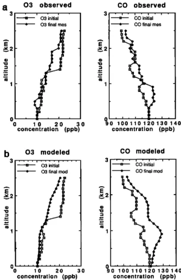
4.3. Comparison Between Modeled and Observed Profiles

Figure 10 displays a comparison between modeled and mea-

sured profiles at the end of cloud convection. There is a stan-

dard deviation of about 10% between the modeled and mea-

sured profiles for both CO and 03. The modeled profiles are more smoothed than experimental ones. In our model we have taken into account the dynamical, microphysical, gas and aque- ous chemistry processes but not the uptake by the forest can-

opy.

During the shallow convection, cumulus cell can mix both layers (fossil and underlying mixing layer) so that the fossil mixed layer is destroyed. For 0 3 the profile is simply linearized

within the cloud as well as below the cloud. The in-cloud

smoothing is obviously driven by the vertical speeds which are very high in this zone. For CO the source is supplied by the rain forest canopy, and its profile is linearized only within the cloud.

When the convection vanishes, in this subcloud layer, two weak cells of convection, in-cloud (moist) and subcloud (dry), are modeled and can explain the different behaviors of CO and 03 near surface. The strength of dynamical processes decays

near the ground surface. The lower cell below 1000 m is

capped by an inversion layer. This features explain the CO accumulation at 800 m, obvious in the profile (Figure 10).

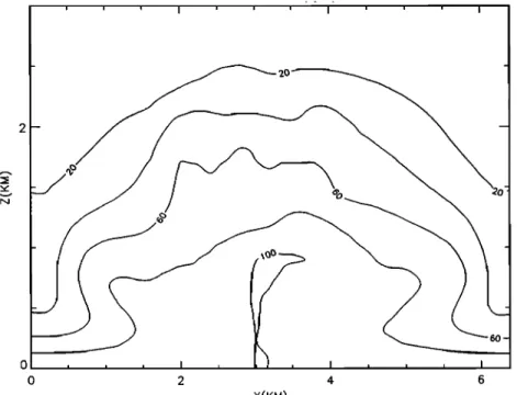
4.4. Inert Tracer Study

A layered tracer scheme is used to investigate the transport

efficiency of a shallow convection cloud field. At initial time an

inert tracer layer is introduced into the model domain between surface and 500 m. At the end of simulation (140 min) we see (Figure 11) that the inert tracer has propagated up to 2000 m.

Forty percent of the initial concentration reaches 2.0 km in

altitude over 2 km wide for a 6.4-km simulated domain in the

horizontal. The compounds lying near surface can be trans- ported above boundary layer, in the free troposphere by a fair-weather cumulus. Several studies have been performed for deep and organized cloud convection, in particular squall lines in Amazonia. A squall line is divided into two components: convective and stratiform. These two regions contribute to vertical transport [Houze, 1989]. Thirty to fifty percent of the vertical transport is accomplished by the hot towers (convec- tive region), and the remainder is brought about the trailing stratiform region which also participates to transport in the upper troposphere by anvil region [Greco et al., 1994]. Simu- lated results (tracer 2 [Scala et al., 1990]) for a squall line show

that 40% of initial concentration reaches 3.5 km over 10 km

wide and only 2.0 km in altitude over 30 km wide for 160 km simulated domain. Therefore, in a squall line, although vertical transport can be observed up to the upper troposphere, a large amount of surface tracer reaches only 2000 m. The squall lines cover large areas, but these meteorological events have a rare occurrence on the overall year. If we examine the lower tro- posphere where the biogenical emissions take place, the shal- low convection plays a role which must be taken into account. It is quite realistic to hypothesize that, even though fair-

weather cumulus induces weaker vertical fluxes than squall

lines, they are more frequent and can contribute to nonnegli- gible amounts of net vertical transport of some surface trace

compounds in lower troposphere (from surface to 2000 m).

4.5. Main Processes Driving the Chemical In-cloud Species Redistribution

Sensitivity tests have been performed to evaluate the relative importance of different processes (transport, photochemistry or aqueous chemistry) on chemical species distribution due to the presence of small cumulus.

2.O 1.5 1.0 0.5 0.0 0 1.0 0.5 - 0.0 0 Time=30 Minutes U m/s W m/s a ß

,-"'•.rS•,-•

.-'--•

"':':•:':':':':'•:'•:':':':'-":':'-':':::::::

... :

mox- &52•20min -,I.75540

Time=50 U m/s 2 ,t. 6 X(KU) max- 2.97880min -3.44650 2.O 0.5 •'.. :.\... ,':..' .

...

ß

-'

.:

...

.'.

...

:

•.'•-•1

• •

i;•

:•.'..:.

•

QCW g/kg

Figure 7. Isolines of horizontal wind, U in meters per second, vertical wind, W in meters per second and cloud liquid water content, QCW in grams per kilogram at different times of the simulation.

cloud water liquid content

1,5

i i i J•

i

0 i ! i ! ! i i ! ß i ! ! !

time (min)

vertical wind speed

6

-2 o e• ,r

time (min)

Figure 8. At 1500 m in center of convection, time evolution

during 140 min, of cloud liquid water content (grams per ki- logram), of vertical speed (meters per second).

initial value in center of cloud are examined (Figure 12). Curve 1 describes the complete scheme which takes into account all the processes: dynamical, microphysical, and chemical. If the aqueous chemical reactions and the transfer between aqueous and gaseous phases are neglected, the CO concentration is not

modified, because it is not soluble, so that curve 2 is not

different from curve 1. For 03 there is a very low increase associated with low 03 solubility and 03 destruction by aque- ous chemistry process. These effects remain unimportant. We notice that the increase in 03 follows the liquid water content maximum (condensation), while the decrease of 03 follows the liquid water content minima (evaporation). For curve 3, we also neglect the dynamical processes, only the gaseous chem-

ical reactions are taken into account like in a box model. In this

case, the CO and 03 concentrations do not vary.

a 0 0 03 observed • 03 initial ß 03 final mes 10 20 30 concentration (ppb) CO observed • •O'init'ial' ' ' * CO final mes ß i . 90 100 110 120 130 140 concentration (ppb) b 03 modeled • • initial ; 03 final mod 10 20 30 concentration (ppb) CO modeled • [;O'initial * CO final mod 0 100110120130140 concentration (ppb)

Figure 10. 03 and CO species mixing ratio profiles (a) ob- tained during the experiment before and after the presence of cloud and (b) obtained by the simulation after the presence of

cloud.

For this kind of cloud (fair-weather cumulus), with low val- ues in NO and 03 concentration, CO and 03 behave like inert gases. Photochemistry represents a very low sink for 03 [Scala et al., 1990]. This phenomenon can be explained as follows: first, CO gas reacts very little with other gases which are in the

2 o 1.8 m 16 •_. . e 1.4 o • 1.2 o o 1 ..,. • 0.6 "' 0.4 0.2

•

CO

ALL

PROCESSES

I

Figure 9. At 1500 m in center of convection, time evolution during 140 min, of 03 and CO concentration

20

0 ,

0 2 4 6

X(KM)

Figure 11. The simulated modification of an inert tracer by cloud transport after 140 min. The initial

distribution lies between surface and 500 m.

atmosphere, and moreover, CO concentration is ten times

greater than other gases, including 03. The evolution of CO and 03 concentration profiles are out of phase: CO increases with height, while 03 decreases. The vertical cloud transport is the main process driving chemical species redistribution. We see that even fair-weather cumulus perform transport or trans-

formation.

5. Evaluation of Cumulus Venting Over a

Tropical Rain Forest During the Wet Season

A survey of shallow (fair-weather) cumulus clouds over part of Amazonia yields to evidence of enhanced frequency of oc- currence of clouds over zone (in particular along the highway) where the forest had been cleared during the 1988 dry season

[Cutrim et al., 1995]. This may be explained by the great con- trast in vegetation cover (deforested areas) that leads to con-

vective motions and therefore shallow cumulus clouds. This is

a permanent feature (during wet or dry season).

The boundary layer in wet season over tropical rain forest is not a source for ozone like in a polluted atmosphere but rather a sink [Ritter et al., 1990; Browell et al., 1990]. Between the boundary layer and the free troposphere, weak cumulus can take place and allow the vertical transfer of chemical species such as CO or 03. These species play a important role in global tropospheric chemistry, and we must estimate the venting in all conditions (here there is shallow convection, above rain forest during the wet season).

In our study, the cloud transforms the fossil layer below 1500 m during the cloud development and "vents" a part of

2 o 1.6 ...,. • 1.4 o 1.2 o 1 • 0.8 N .=,., E O.6 • 0.4 0.2

TIME EVOLUTION FOR GAS PHASE CONCENTRATIONS

C:) C:) C:) C:) C:) C:)

0,1 'q' •.0 1:0 0 0,1

time (mini

Figure 12. At 1500 m in center of convection, time evolution during 140 min of 03 (dotted line) and CO (solid line) concentration normalized by initial value. Run 1' All the processes (dynamical, gas, and aqueous phases) are taken into account. Run 2: no transfer through the aqueous phase. Run 3: only gas chemistry.

content above 2000 m into the free troposphere. We evaluated during the whole simulation the CO and 0 3 fluxes between the

boundary layer at 1500 m and the free troposphere toward the

cloud top. We have calculated the CO and 0 3 net vertical fluxes between these levels. The CO and 0 3 upward fluxes are

respectively

7.7 x 1023

molecules

km -2 h -1 and 1.2 x 1023

times smaller than those obtained for O 3 during deep convec- tion (PRESTORM), with high value of NO, which are 7.97 x 10 TM molecules cm -2 s -1, that is 2.8 x 1025 molecules km -2

h -• [Pickering et al., 1992; Thomson et al., 1994]. In addition,

we see that the CO vertical transport is negligible versus 0 3

transport.

6. Conclusions

We have presented a cloud convection model coupled with a chemical model describing the oxidation chains of CH 4 and

CO in presence of NOx in remote troposphere. A shallow cumulus cloud field has been simulated over tropical rain for-

est, during the wet season, with low values of 03 and NOx. The case under study represents a local system which includes an active mixing layer from surface to 1000 m capped by a fossil

mixed layer between 1000 and 1500 m, cumulus clouds pene-

trate into this layer and exchanges between the different layers

are examined. We have shown that when vertical motion is

strong, the fossil mixed layer and the mixing layer are mixed so that the fossil layer is destroyed. By tracer analysis, we have shown exchanges exist between the lower layer (from surface to 500 m) and the free troposphere (above 2000 m) across the

mixing and fossil layer. After the development of several cycles of cloud cells, when the cloud precipitates, we have two con- vection cells: the first one from the ground to 1000 m and the

second one from 1300 to 2200 m where is found a cloud cell. At

this time, the exchanges between the two layers are stopped.

The comparison between experimental and modeled CO

and 03 data are in good agreement. The cloud convection smoothes more the 03 vertical profile than the CO one be- cause CO is supplied from ground surface and is therefore

more concentrated near the surface than in altitude, while the

opposite occurs for 03 which is destroyed very weakly within the atmosphere by photochemistry. Sensitivity tests show that the main process driving chemical species redistribution is the dynamical mechanism. The microphysical and chemical pro- cesses are of lower importance. We have shown that even small clouds perform transport or transformation in the boundary

layer.

The 0 3 and CO vertical fluxes between the boundary layer and the free troposphere through the cloud top, are respec-

tively 1.2 x 1023 molecules km -2 h-l and 7.7 x 1023 molecules km -2 h -•. In tropical region, over rain forest, with low 03

levels, where several cumulus exist every day, the vertical fluxes of some chemical species (like 03) cannot be neglected.

Acknowledgments. This study is supported by the "Programme National de Chimie Atmosph6rique" of the CNRS. Computer re- sources were provided by the IDRIS Center (France, project 950187). We thank very gratefully both reviewers for constructive comments and advice, and more particularly the M. Garstang for the helpful information he gave us concerning the ABLE 2B campaign. The au- thors express their gratitude to N. Chaumerliac for her helpful com-

ments.

References

Browell, E. V., G. L. Gregory, R. C. Harriss, and V. W. J. H. Kirchhoff, Ozone and aerosol distribution over the Amazon basin during the wet season, J. Geophys. Res., 95, 16,887-16,902, 1990.

Cautenet, S., and B. Lefeivre, Contrasting behavior of gas and aerosol scavenging in convective rain: A numerical and experimental study in the African equatorial forest, J. Geophys. Res., 99, 13,013-13,024,

1994.

Chameides, W. L., and D. D. Davis, The free radical chemistry of cloud droplets and its impact upon the composition of rain, J. Geo- phys. Res., 87, 4863-4877, 1982.

Chatfield, R. B., and A. C. Delany, Convection links biomass burning to increased tropical ozone: However, models will tend to overpre- dict 03, J. Geophys. Res., 95, 18,473-18,488, 1990.

Chaumerliac, N., R. Rosset, M. Renard, and E. C. Nickerson, The transport and redistribution of atmospheric gases in regions of fron-

tal rain, J. Atmos. Chem., 14, 43-51, 1989.

Ching, J. K. S., and A. J. Alkezweeny, Tracer study of vertical exchange by cumulus clouds. J. Climatol. Appl. Meteorol., 25, 1702-1711, 1986.

Cutrim, E. M. C., D. W. Martin, and R. Rabin, Enhancement of

cumulus clouds over highlands, savannah and deforestation lands in Amazonia, Ann. Geophys., 13, 309, 1995.

Fitzjarrald, D. R., K. E. Moore, O. M. R. Cabral, J. Scolar, A. O. Manzi, and L. D. de Abrau Sa, Daytime turbulent exchange between the Amazon forest and the atmosphere, J. Geophys. Res., 95, 16,825-

16,838, 1990.

Garstang, M., et al., Trace gas exchanges and convective transports over the Amazonia rain forest, J. Geophys. Res., 93, 1528-1550,

1988.

Gidel, L. T., Cumulus cloud transport of transient tracers, J. Geophys.

Res., 88, 6587-6599, 1983.

Graedel, T. E., and P. J. Crutzen, Atmospheric change. An Earth System Perspective, 446 pp., W. H. Freeman, New York, 1993.

Greco, S. R., M. Swap, M. Garstang, S. Ulanski, M. Shipham, R. C.

Harris, R. Talbot, M. O. Andreae, and P. Artaxo, Rainfall and

surface kinematic conditions over central Amazonia during ABLE 2B, J. Geophys. Res., 95, 17,001-17,014, 1990.

Greco, S., J. Scala, J. Halverson, H. L. Massie, W. K. Tao, and M.

Garstang, Amazon coastal sqall lines, II, Heat and moisture trans- ports, Mon. Weather Rev., 122, 623-635, 1994.

Gr6goire, P. J., N. Chaumerliac, and E. C. Nickerson, Impact of cloud dynamics on tropospheric chemistry: Advances in modeling the in- teractions between microphysical and chemical processes, J. Atmos.

Chem., 18, 247-266, 1994.

Harriss, R. C., G. W. Sachse, G. F. Hill, L. O. Wade, and G. L.

Gregory, Carbon monoxide over the Amazon basin during the wet season, J. Geophys. Res., 95, 16,927-16,931, 1990.

Hesstvedt, E., O. Hov, and I. S. A. Isaksen, Quasi-steady-state approx- imations in air pollution modeling: Comparison of two numerical schemes for oxidant prediction, Int. J. Chem. Kinetics, 10, 971-994,

1978.

Houze, R. A., Observed structure of mesoscala convective systems and implications for large-scale heating, Q. J. R. Meteorol. Soc., 487,

425-461, 1989.

Jacob, D. J., Chemistry of OH in remote clouds and its role in the production of formic acid and peroxymonosulfate, J. Geophys. Res.,

91, 9807-9826, 1986.

Jacob, D. J., and S.C. Wofsy, Budgets of reactive nitrogen, hydrocar- bons, and ozone over the Amazon forest during the wet season, J. Geophys. Res., 95, 16,737-16,754, 1990.

Kessler, E., On the redistribution and continuity of water substance in atmospheric circulation, Meteorol. Monogr., 10(32), 84 pp., 1969. Lafore, J.P., and M. W. Moncrieff, A numerical investigation of the

organisation and interaction of the convective and stratiform regions of tropical squall lines, J. Atmos. Sci., 46, 521-544, 1989.

Lelieveld, J., and P. J. Crutzen, Influences of cloud photochemical processes on tropospheric ozone, Nature, 343, 227-233, 1990. Lelieveld, J., and P. J. Crutzen, The role of clouds in tropospheric

photochemistry. J. Atmos. Chem., 12, 229-267, 1991.

Lyons, W. A., R. H. Calby, and C. S. Keen, The impact of mesoscale convective systems on regional visibility and oxidant distribution during persistent elevated pollution episodes, J. Climatol. Appl. Me-

teorol., 25, 1518-1531, 1986.

Madronich, S., Photodissociation in the atmosphere, 1, Actinic flux and the effect of ground reflections and clouds, J. Geophys. Res., 92,

Marshall, J. S., and W. M. Palmer, The distribution of raindrops with

size, J. Meteorol., 5, 165-166, 1948.

Martin, C. L., D. Fitzjarrald, M. Garstang, A. P. Oliveira, S. Greco, and E. Browell, Structure and growth Of the mixing layer over the Am- azonian rain forest, J. Geophys. Res., 93, 1361-1375, 1988. Pickering, K. E., A.M. Thompson, R. R. Dickerson, W. T. Luke, D. P.

McNamara, J.P. Greenberg, and P. R. Zimmerman: Model calcu- lations of tropospheric ozone production potential following ob- served convective events, J. Geophys. Res., 95, 14,049-14,062, 1990. Pickering, K. E., A.M. Thompson, J. R. Scala, W. K. Tao, J. Simpson,

and M. Garstang, Photochemical ozone production in tropical squall line convection during NASA Global Tropospheric Experiment/ Amazon Boundary Layer Experiment 2A, J. Geophys. Res., 96,

3099-3114, 1991.

Pickering, K. E., A.M. Thompson, J. R. Scala, W. K. Tao, R. R. Dickerson, and J. Simpson, Free tropospheric ozone production following entrainment of urban plumes into deep convection, J. Geophys. Res., 97, 17,985-18,000, 1992.

Preiss, M., R. Maser, H. Franke, W. Jaescke, and J. Graf, Distribution of trace substances inside and outside of clouds, Beitr. Phys. Atmos.,

6 7, 341-351, 1994.

Renard, M., N. Chaumerliac, S. Cautenet, and E. C. Nickerson, Tracer redistribution by clouds in West Africa: Numerical modeling for dry and wet seasons, J. Geophys. Res., 99, 12,873-12,883, 1994. Ritter, A. J., D. H. Lenschow, J. D. W. Barrick, G. L. Gregory, G. W.

Sachse, G. F. Hill, and M. A. Woerner, Airborne flux measurements and budget estmates of traces species over the Amazonian basin during the GTE/ABLE2B Expedition, J. Geophys. Res., 95, 16,875-

16,886, 1990.

Scala, J. R., Cloud draft structure and trace gas transport, J. Geophys.

Res., 95, 17,015-17,030, 1990.

Singh, H. B., D. Herlth, D. O'Hara, L. Salas, A. L. Torres, G. L. Gregory, G. W. Sachse, and J. F. Kasting, Atmospheric peroxyacetyl nitrate measurements over the Brasilian Amazon basin during the wet season: Relationships with nitrogen oxides and ozone, J. Geo- phys. Res., 95, 16,945-16,954, 1990.

Stockwell, W. R., Communication to the Editor regarding "Lelieveld, J., and P. J. Crutzen, 1991: The role of clouds in tropospheric photochemistry, J. Atmos. Chem., 12, 229-267, 1994.

Talbot, R. W., M. O. Andreae, H. Berresheim, D. J. Jacob, and K. M.

Beeker, Sources and sinks of formic, acetic and pyruvic acids over central Amazonia, 2, Wet season, J. Geophys. Res., 95, 16,799-

16,811, 1990.

Thompson, A. N., K. E. Pickering, R. R. Dickerson, W. G. Ellis Jr., D. J. Jacob, J. R. Scala, W-K Tao, D. P. McNamara, and J. Simpson, Convective transport over the central United States and its role in regional CO and ozone budgets, J. Geophys. Res., 99, 18,703-18,711,

1994.

P. Br•maud, Laboratoire de Physique Atmosphere, Universite de

l'ile de la Reunion, St. Denis, 95 France.

S. Cautenet and J. Edy, Laboratoire de Meteorologie Physique, Universite Blaise Pascal/CNRS, 24 Avenue des Landais, 63177

Aubi•re, France.

(Received June 13, 1995; revised May 20, 1996; accepted May 25, 1996.)