Development and Evaluation of Speech Privacy Measurement Software: SPMSoft

(1)

Publisher’s version / Version de l'éditeur:

Vous avez des questions? Nous pouvons vous aider. Pour communiquer directement avec un auteur, consultez la

première page de la revue dans laquelle son article a été publié afin de trouver ses coordonnées. Si vous n’arrivez pas à les repérer, communiquez avec nous à PublicationsArchive-ArchivesPublications@nrc-cnrc.gc.ca.

Questions? Contact the NRC Publications Archive team at

PublicationsArchive-ArchivesPublications@nrc-cnrc.gc.ca. If you wish to email the authors directly, please see the first page of the publication for their contact information.

https://publications-cnrc.canada.ca/fra/droits

L’accès à ce site Web et l’utilisation de son contenu sont assujettis aux conditions présentées dans le site LISEZ CES CONDITIONS ATTENTIVEMENT AVANT D’UTILISER CE SITE WEB.

Research Report (National Research Council of Canada. Institute for Research in Construction), 2008-08-01

READ THESE TERMS AND CONDITIONS CAREFULLY BEFORE USING THIS WEBSITE. https://nrc-publications.canada.ca/eng/copyright

NRC Publications Archive Record / Notice des Archives des publications du CNRC : https://nrc-publications.canada.ca/eng/view/object/?id=0f0fc86e-e4ad-456e-ad83-a7db8d495415 https://publications-cnrc.canada.ca/fra/voir/objet/?id=0f0fc86e-e4ad-456e-ad83-a7db8d495415

NRC Publications Archive

Archives des publications du CNRC

For the publisher’s version, please access the DOI link below./ Pour consulter la version de l’éditeur, utilisez le lien DOI ci-dessous.

https://doi.org/10.4224/20377879

Access and use of this website and the material on it are subject to the Terms and Conditions set forth at Development and Evaluation of Speech Privacy Measurement Software: SPMSoft

(2)

http://irc.nrc-cnrc.gc.ca

D e v e l o p m e n t a n d E v a l u a t i o n o f S p e e c h

P r i v a c y M e a s u r e m e n t S o f t w a r e : S P M S o f t

R R - 2 6 2

Bradley, J.S.; Gover, B.N.

A u g u s t 2 0 0 8

The material in this document is covered by the provisions of the Copyright Act, by Canadian laws, policies, regulations and international agreements. Such provisions serve to identify the information source and, in specific instances, to prohibit reproduction of materials without written permission. For more information visit http://laws.justice.gc.ca/en/showtdm/cs/C-42

Les renseignements dans ce document sont protégés par la Loi sur le droit d'auteur, par les lois, les politiques et les règlements du Canada et des accords internationaux. Ces dispositions permettent d'identifier la source de l'information et, dans certains cas, d'interdire la copie de documents sans permission écrite. Pour obtenir de plus amples renseignements : http://lois.justice.gc.ca/fr/showtdm/cs/C-42

(3)

Development and Evaluation of Speech

Privacy Measurement Software: SPMSoft

John S. Bradley and Bradford N. Gover

IRC Research Report, IRC RR-262

August 2008

(4)

Acknowledgements

The SPMSoft program was initially created by Darren Ronda while he was working as a coop-engineering student at the Institute for Research in Construction at the National Research Council. Further improvements have been made by Sebastian Schmidt and Timothy Estabrooks.

The work was jointly funded by PWGSC and NRC and was a part of a project to develop new software to facilitate the measurement of speech privacy in open-plan offices.

(6)

1. Introduction

Adequate speech privacy in open-plan offices is difficult to achieve and requires careful attention to the details of the office design [1-3]. Traditionally, objective measurements to evaluate the speech privacy between workstations in open-plan offices have required time-consuming measurements. These included measuring the attenuation of sound between pairs of locations in the office in unoccupied conditions as well as daytime measurements of typical ambient noise levels to make possible the calculation of speech privacy measures. Such tests are complicated, expensive and hence are rarely carried out. The SPMSoft program was developed to make speech privacy measurements in open-plan offices more convenient. The program measures attenuations; ambient noise levels and calculates privacy measures while on site at each location in the office. SPMSoft allows accurate measurements of speech privacy in open-plan offices during normal working hours. This provides a precise rating of the existing conditions for comparison with more ideal (but achievable) goals. The program also provides information to help the user identify the primary causes where the speech privacy is less than desired. It is hoped that using SPMSoft to better understand speech privacy problems will lead to better solutions to these problems.

This report documents various tests to evaluate the performance of SPMSoft. This includes validation tests of each component of the measurements and evaluation of the repeatability of the results. Further sections give help for interpreting the measurement results and advice for optimizing the quality of each measurement. A companion document [4] describes the results of various measurement case studies showing the effects of key design parameters on measured conditions in various offices. The case study results provide advice as to the expected results in various types of real open-plan offices.

In North America, speech privacy has been measured in terms of values of the

Articulation Index (AI) [5, 6]. Values of AI ≤ 0.15 have been said to provide ‘normal’ privacy for an open-plan office [7]. More recently the Speech Intelligibility Index (SII) [8] has replaced AI in the ANSI standard. In terms of SII values, an SII ≤ 0.20

corresponds to ‘normal’ speech privacy. Both AI and SII are frequency weighted signal-to-noise ratios with the signal-signal-to-noise ratio in each 1/3-octave band limited to a range of 30 dB.

One calculates AI or SII from the speech and noise levels at each receiver location. The ambient noise levels are measured in 1/3-octave bands. The attenuation of sound between the source position and the receiver position is also measured in 1/3-octave bands. By subtracting the measured attenuations from a standard voice spectrum for a position 1 m from the talker, the speech level at the receiver position is determined. The AI or SII are then calculated from the measured ambient noise and the expected received speech levels.

In Europe, there are proposals to use the Speech Transmission Index (STI) to measure speech privacy in open-plan offices [9]. STI can be calculated from the complete impulse response measured between the source and receiver location along with the speech and noise levels at the receiver position [10]. STI reflects the effect of signal-to-noise and reverberation on the intelligibility of speech. SPMSoft also measures STI values.

(7)

2. Description of Software

(a) Program overview

This section gives a brief overview of the SPMSoft program so that the reader can better understand the results of the various evaluation tests of the software. The SPMSoft program was designed to make it possible to efficiently measure speech privacy between locations in open-plan offices. The program uses a high quality sound card to output a sine sweep test signal to a power amplifier and loudspeaker while simultaneously capturing the response via a microphone connected to the sound card input. The impulse response of the transmission from the source position to the receiver position is

calculated and the ambient noise levels are recorded so that indicators of speech privacy can be determined.

Figure 1 shows the main measurement window of the SPMSoft program with an example measurement result. The upper half of the screen shows the measured ambient noise levels displayed as octave band levels indicated by the red bars over the NC, NCB or RC contours in the background. Although displayed as octave band levels, the measured ambient noise is first filtered into 1/3-octave bands, and 1/3-octave band levels are saved with other results in a *.csv file for each measurement. The measured ambient noise is the

result of integrating over a user specified duration, which would usually be 20 to 30 s.

Envelope

(8)

The lower half of the screen includes a plot of the measured impulse response (IR) displayed as the envelope of the impulse response. This is obtained by calculating the Hilbert transform of the impulse response and then determining the envelope of impulse response. The impulse envelope provides a clearer picture of the main events in the impulse response and makes it possible to plot the amplitude in decibels. In SPMSoft the first 70 ms of the impulse response envelope is displayed. The blue and red boxes on the impulse response plot are calculated from the dimensions of the measured workstations provided by the user. The blue box indicates the expected time of arrival of the initial sound diffracted over the separating panel. The red box indicates when the initial ceiling reflection is expected to arrive. The amplitudes of the peaks within these boxes indicate their relative importance for reducing speech privacy. If the peaks in the red box are higher, the ceiling reflection is dominant and one should first increase the ceiling

absorption to improve speech privacy. However, if the peaks in the blue box are higher, it is most important to raise the height of the separating workstation panel to improve speech privacy.

The program functions by the user pushing each of the rectangular buttons on the upper left part of the screen in sequence. This causes the program to go through the steps of making a measurement in the appropriate order. Buttons are greyed out when it is not appropriate to select them. Thus the user normally: (a) starts a new measurement, (b) calibrates the microphone, (c) measures the ambient noise level, (d) measures the impulse response (e) calculates results, (f) enters the information to determine the ‘diagnostic’ boxes plotted on the impulse response, and then (g) can optionally print a report or save the results to file.

The microphone must be calibrated before any measurements can be made so that the measured voltages can be converted to absolute sound pressures in pascals. Figure 2 illustrates the calibration screen, showing a simple graph with 3 horizontal lines. The two red lines are reference lines. A successful calibration will produce a smooth horizontal blue line between the two red lines. If the blue line is not smooth the calibration tone was not constant during the calibration and it should be repeated. If the blue line is below the two red lines, the measurement hardware should include more amplification between the microphone and the sound card. If the blue line is above the red lines, less amplification is required.

(9)

The program measures the attenuation between the source and the receiver from the measured impulse response. The 1/3-octave band levels of the tests signal, measured at the receiver position, are subtracted from the reference values, measured at a distance of 1 m in a free field such as an anechoic room, to obtain attenuation values. Then

attenuations are subtracted from the assumed speech source levels in each 1/3-octave band to calculate the expected speech levels at the receiver position. From these received speech levels and the measured ambient noise levels, the signal-to-noise ratio measures AI (Articulation Index) [5] and SII (Speech Intelligibility Index) [8] are calculated. The calculation of STI (Speech Transmission Index) is more complex and involves Fourier transformation of the squared octave band impulse responses. The matrix of modulation reductions that are obtained from this process are then combined with the received speech spectrum and the measured ambient noise spectrum to calculate STI [10].

Figure 3 shows the source reference level measurement screen. This is used to measure the reference sound levels of the sine sweep signal at a distance of 1 m in a free field such as an anechoic room. When such free field conditions are not available the program allows the user to select a restricted 5 ms time window for the reference source level measurement. Measurement of the reference sound levels are then possible with the source and receiver 1 m apart in a large room with the source and receiver at least 2 m from all reflecting surfaces.

Figure 3. SPMSoft reference sound level measurement window. (b) Program details

This section includes reference information about the details of the SPMSoft program. It is not necessary to read this section to understand the following sections and it can be skipped over until these details are needed.

(10)

Sine sweep signal and the impulse response. The SPMSoft program includes a sine sweep signal in a wav file format and named ‘Opink_80_10k_18_44100.wav’ as well as an inverse file named ‘Opink_80_10k_18_44100.inv’. The sine sweep file was created outside of the program. It has a pink spectrum shape extending from 80 to 10,000 Hz obtained by using a logarithmic time sweep rather than varying the amplitude. It is 218 samples long at a sampling rate of 44,100 samples per second and hence each sweep lasts 5.94 s. The inverse file when transformed into the frequency domain corresponds to the inverse filter to the spectrum of the sine sweep signal. Impulse responses are calculated by multiplying the inverse filter by the recorded response in the frequency domain and then inverse transforming the result to give the impulse response between the source loudspeaker and the microphone. The impulse response has a duration of 5.94 s.

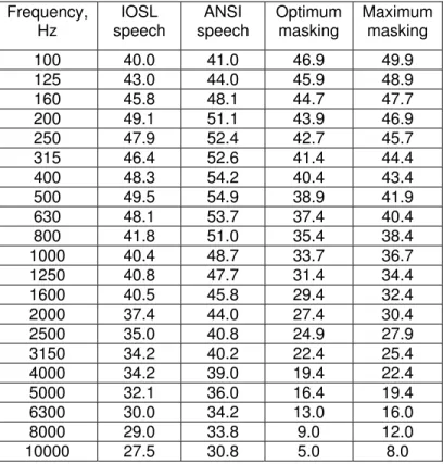
Input speech and noise data. SPMSoft includes 1/3-octave band values of speech and noise spectra that can be selected for use in calculations. These are listed in Table 1.

Frequency, Hz IOSL speech ANSI speech Optimum masking Maximum masking 100 40.0 41.0 46.9 49.9 125 43.0 44.0 45.9 48.9 160 45.8 48.1 44.7 47.7 200 49.1 51.1 43.9 46.9 250 47.9 52.4 42.7 45.7 315 46.4 52.6 41.4 44.4 400 48.3 54.2 40.4 43.4 500 49.5 54.9 38.9 41.9 630 48.1 53.7 37.4 40.4 800 41.8 51.0 35.4 38.4 1000 40.4 48.7 33.7 36.7 1250 40.8 47.7 31.4 34.4 1600 40.5 45.8 29.4 32.4 2000 37.4 44.0 27.4 30.4 2500 35.0 40.8 24.9 27.9 3150 34.2 40.2 22.4 25.4 4000 34.2 39.0 19.4 22.4 5000 32.1 36.0 16.4 19.4 6300 30.0 34.2 13.0 16.0 8000 29.0 33.8 9.0 12.0 10000 27.5 30.8 5.0 8.0

Table 1. Speech source levels in decibels (at 1 m in a free field) and noise levels all in 1/3-octave bands that are included in SPMSoft.

The speech levels at the receiver position are calculated by first selecting a speech source level (measured at 1 m in a free field) and reducing the levels in each band according to the measured attenuations to the receiver location. Table 1 includes 2 different speech source level spectra that can be used or alternatively the user can enter their own speech spectrum for special calculations. The included speech spectra are the Intermediate Office Speech Level (IOSL) obtained from measurements of voice levels in open-plan offices and intended for open-plan office design calculations [2,3]. The ‘normal’ speech levels included in the ANSI S3.5 standard are also included to make it possible to produce

(11)

results based on this standard spectrum. However, it is highly recommended that the IOSL speech spectrum be used to most accurately estimate the privacy conditions in open-plan offices. The ANSI spectrum is much louder than people typically talk in open plan offices [11].

Table 1 also includes 2 different ambient noise spectra. Using one of these noise spectra or a user defined noise spectrum makes it possible to obtain realistic results when representative ambient noise levels do not exist or to compare offices with exactly the same ambient noises.

The Optimum masking noise spectrum has an overall level of 45 dBA that was judged to be an optimum masking level [2,3,12]. The Maximum masking level corresponds to approximately 48 dBA. Above this level ambient noise or masking noise cause increased annoyance and cause occupants to talk more loudly, defeating the benefit of its masking properties [13]. The user can also enter their own ambient noise spectrum.

Source level measurements and calculations. SPMSoft uses the levels of the test signal measured at 1 m in a free field to calculate attenuations to receiver positions in open-plan offices. As illustrated in Figure 3, the measured reference levels are displayed on the measurement screen after adjusting them to be representative of a 0 dB output signal level. That is, if the reference levels at 1 m were measured using a –15 dB output level, the numbers on the screen would be 15 dB higher than the actual measured levels. The levels are based on integrations over the complete 5.94 s of the measured impulse responses and hence the peak levels at each frequency would be higher.

The measured levels are stored as sound power levels and converted back to levels at 1 m when they are used in measurements. In a free field, sound pressure levels, Lp, are related

to sound power levels, Lw, for a point source as follows,

Lp = Lw +10 log{1/(4πr2)}, dB (1)

Where r is the source-receiver distance in m. In our case r = 1.0 and equation (1) becomes,

Lp = Lw+11, dB

Output data file. The main results of the SPMSoft measurements are output to a *.csv

format file that is easily read and further processed in spreadsheet software. Table 2 lists the contents of the output *.csv file as recorded from left to right in this file.

Output of IR to file. The first 70 ms of the envelope of the Impulse Response (IR) displayed on the main measurement screen can be output to a *.csv format file for

plotting and inclusion in reports. This feature is found as an option under the File Menu.

Source sound power level file.

The measured source levels at 1 m in a free field are saved as sound power levels as described above. The 1/3-octave band sound power levels are in files with the name, ‘Opink_80_10k_18_44100_nn.tlw’, where ‘nn’ is an integer that is incremented each time a new reference sound level measurement is made. The initial part of the name is the same as the sine sweep file name so that they are always connected. The *.tlw files are

(12)

Content Description

STI Average

Speech Transmission Index calculated as the average of the results using the frequency weightings for male and female talkers.

STI Female

Speech Transmission Index calculated using frequency weightings for female talkers.

STI Male

Speech Transmission Index calculated using frequency weightings for male talkers.

AI Articulation Index (ANSI S3.5 (1969))

SII Speech Intelligibility Index (ANSI S3.5 (1997)) S/N(A) A-weighted speech level - A-weighted noise level.

U50 Useful-to-Detrimental sound ratio (Experimental, not validated) Source Width Width of the source workstation (m)

Receive Width Width of the receiving workstation (m) Ceiling Height Height of the office ceiling (m)

Screen Height Height of the separating panel (m)

Source Distance Distance of source (m) from separating panel Microphone

Distance

Distance of the microphone (m) from separating panel Loudspeaker Height Height of the loudspeaker (m)

Microphone Height Height of the microphone (m) Ceiling Text describing the office ceiling Screen Text describing the workstation panels Walls Text describing the office walls

Noise levels 1/3 octave band noise levels used in the measurement from 50 Hz to 10,000 Hz plus the overall A-weighted noise level.

Attenuations levels Measured attenuations in 1/3-octave bands from 100 to 10,000 Hz plus the overall A-weighted attenuation.

Voice spectrum Speech source levels used in the measurement from 100 to 10,000 Hz plus the overall A-weighted level.

Sound power level 1/3-octave band sound power levels of the test source from 100 to 10,000 Hz plus the overall A-weighted level. These are obtained from the measured on-axis levels of the test source at a distance of 1 m in a free field.

Sensitivity Microphone sensitivity in units (of digitized signal) per pascal SNRSII22 Uniform weighted signal to noise ratio (Experimental, not

validated)

SNRUNI32 SII weighted signal to noise ratio (Experimental, not validated) Table 2. Description of content of output *.csv format data file.

(13)

3. Validation Tests

This section includes summary results of various tests to validate each component of the SPMSoft program including comparisons with the results of conventional measurements of open-plan office speech privacy.

(a) 1/3-octave band filters.

The recorded ambient noise and measured attenuations both include filtering into 1/3-octave bands. The 1/3-1/3-octave filters comply with the requirements of ANSI S1.11 [14] for the 1/3-octave bands required in the speech privacy measures. Figure 4 shows the measured response of the 1000 Hz 1/3-octave band filter, which is seen to fall within the acceptable range of characteristics required by ANSI.

500 1000 1500 2000 30 40 50 60 70 80 90 Level , dB Frequency, Hz

Figure 4. Measured response of 1000 Hz 1/3-octave band filter (solid line) and the allowed range of characteristics according to ANSI S1.11 (dashed lines).

100 1000 10000 20 40 60 80 100 Le ve l, dB Frequency, Hz

(14)

The responses of all of the 1/3-octave band filters from 50 Hz to 10,000 Hz are plotted in Figure 5. There are substantial irregularities in the lowest frequency filters and especially the 50 and 63 Hz filters. However, only the 1/3-octave band filters from 160 Hz to 8,000 Hz are required for the speech privacy measures AI(200-5k) and SII(160-8k). The filters for these 1/3-octave bands fall within the ANSI requirements. STI uses the octave band filtered impulses responses from 125 to 8k Hz.

(b) Ambient noise level measurement

Measured ambient noise levels using SPMSoft and including these same filters were compared with simultaneous measurements using a Bruel and Kjaer type 2144 analyser. An example of these comparisons is shown in Figure 6. In this case the difference between the two measurements varies from –0.09 dB to +0.32 dB over the range from 160 Hz to 8k Hz. The average of the absolute value of the differences was 0.12 dB with a standard deviation of ±0.083 dB. A number of similar results served to confirm the acceptability of the 1/3-octave band filters used and the related calculations in the SPMSoft program. 125 250 500 1000 2000 4000 8000 10 15 20 25 30 35 40 SPL, dB Frequency, dB

Figure 6. Comparison of simultaneous ambient noise measurements using SPMSoft and a Bruel and Kjaer type 2144 analyser.

(c) Attenuation measurement

SPMSoft measures sound propagation in terms of the attenuation between the reference 1/3-octave band source levels measured 1 m from the source loudspeaker on axis in a free field and the measured levels in the receiver workstation. Such attenuations can also be measured using a steady state test signal such as pink noise. The results of such

conventional measurements were compared with the SPMSoft attenuations to validate the new software. For the pink noise the source levels at 1 m were measured in an anechoic room and new measurements were made in a receiving workstation to provide attenuation values in the 1/3-octave bands from 100 Hz to 10 kHz. These attenuations were

(15)

Figure 7 shows an example of these comparisons. In Figure 7 the differences between the two results varied form –0.69 to +0.38 dB with a standard deviation of ±0.305 dB

between 100 and 8k Hz. 0 5 10 15 20 25 30 125 250 500 1000 2000 4000 Frequency, Hz Attenuati on, dB Conventional SPMSoft

Figure 7. Comparison of attenuation measurements using SPMSoft and a Bruel and Kjaer type 2144 analyser and a pink noise signal.

(d) Measurement of speech privacy parameters

The complete speech privacy measurement process can be checked by comparing the AI values measured with SPMSoft with parallel measurements using a conventional

approach. Pink noise signals and a Bruel and Kjaer type 2144 1/3-octave band analyser were used to measure attenuations as well as ambient noise levels and AI values were calculated from these results. Figure 8 compares the resulting AI values from a series of 6 measurements for varied source and receiver position in a pair of adjacent workstations. In Figure 8 the vertical scale deliberately exaggerates the small differences. The average of the absolute value of the differences in AI values for these results was 0.0043 with a standard deviation of ±0.0020. The comparison of SII values for these same cases indicated an average of the absolute value of the differences of 0.0030 with a standard deviation of ±0.0015. The results for SII values are included in Figure 9.

(16)

1 2 3 4 5 6 0.20 0.25 0.30 AI Position AI Conventional AI SPMSoft

Figure 8. Comparison of AI values measured using SPMSoft with conventional measurements (mean absolute value of differences 0.0043, standard deviation

±0.0020). 1 2 3 4 5 6 0.25 0.30 0.35 SII Position SII Conventional SII SPMSoft

Figure 9. Comparison of SII values measured using SPMSoft with conventional measurements (mean absolute value of differences 0.0030, standard deviation ±0.0015).

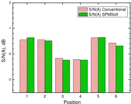
Figure 10 shows a similar comparison for A-weighted speech - noise level differences (S/N(A)). For these data the average of the absolute value of the difference was only -0.056 dB with a standard deviation of ±0.0376 dB. The errors are presumably small because A-weighting reduces the importance of the lower frequencies where differences

(17)

tend to be a little larger. (However, S/N(A) values are not a good predictor of speech intelligibility and speech privacy).

1 2 3 4 5 6 -3 -2 -1 0 Position S/ N (A ), dB S/N(A) Conventional S/N(A) SPMSoft

Figure 10 Comparison of S/N(A) values measured using SPMSoft with those values from conventional measurements (mean of absolute value of the differences 0.056 dB, standard deviation ±0.0376 dB).

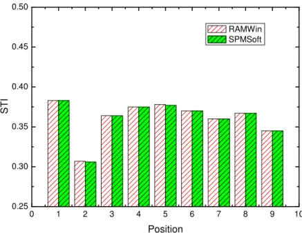
Nine measurement conditions were also used to compare calculated STI values from SPMSoft with STI values using our room acoustics measurements software RAMWIN. Because some of the program elements used by RAMWIN are the same as those in SPMSoft this is not a perfect comparison of independent measurement systems. However, the STI values obtained by the RAMWIN software were previously successfully compared with those from the MLSSA software and an independent MATLAB routine. Both SPMSoft and RAMWIN obtain a matrix of modulation reduction values from a measured impulse response. These are then combined with measured speech and noise levels to calculate STI values.

Figure 11 compares the STI values from the two programs. For these nine measurement conditions, the mean of the absolute differences was –0.00036 and the standard deviation of the differences was ±0.000359.

In all cases the differences between the two compared approaches are very small and might be further reduced by using increased signal levels and more averaging when using SPMSoft. These results confirm that SPMSoft speech privacy measurements accurately reproduce conventional measurements.

(18)

0 1 2 3 4 5 6 7 8 9 10 0.25 0.30 0.35 0.40 0.45 0.50 STI Position RAMWin SPMSoft

Figure 11 Comparison of STI values measured using SPMSoft with those values using from the RAMWIN room acoustics measurement software (mean of absolute differences -0.00036, standard deviation ±0.000359).

(19)

4. Calibration of source output

SPMSoft requires that the source output be calibrated by measuring the source levels at 1 m in a free field such as in an anechoic room. This makes it possible to measure only the strength of the direct sound without the additional contributions of reflected energy. As users of SPMSoft may not have access to an anechoic room, other techniques were investigated that might provide a more convenient method for measuring the level of the test signal at 1 m without the influence of reflected sound.

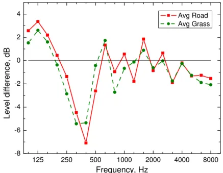
The first approach was to locate the source on the ground outdoors pointing upwards and far from any other reflecting surfaces. This was tried on both asphalt (a road) and a rough grass surface. Several measurements were made and the results averaged to minimize unwanted noise effects. The differences between these measured source levels and others obtained in an anechoic room are compared in Figure 12. There are large differences of several decibels. Such outdoor measurements were concluded to be unacceptable.

125 250 500 1000 2000 4000 8000 -8 -6 -4 -2 0 2 4 Le v e l dif fe ren c e , d B Frequency, Hz Avg Road Avg Grass

Figure 12. Differences between outdoor measurements of SPMSoft source levels over road or rough grass surface relative to those in an anechoic room.

A second approach was to include the capability of measuring the source levels in an ordinary large room by time-windowing the impulse response to eliminate unwanted reflections in the measured response. This process was evaluated to determine how closely the measured source levels in an ordinary room agreed with those obtained in an anechoic test room. Initial tests produced some quite large differences between the time windowed results in an ordinary large room and those in an anechoic room as illustrated in Figure 13. However, these large low frequency differences were shown to be due to the characteristics of the 1/3-octave band geometric equalizer used to correct the loudspeaker response. Depending on the particular equalization used, the transient response of some of the lower frequency 1/3-octave band filters delayed significant amounts of energy so that it arrived after the 5 ms time window.

(20)

63 125 250 500 1000 2000 4000 8000 -10 -8 -6 -4 -2 0 2 4 6 8 10 Leve l di fferen ce, dB Frequency, Hz

Figure 13. Differences between SPMSoft source levels measured by time windowing responses in an ordinary large room and those obtained in an

anechoic room, which were caused by using two different settings of a geometric equalizer.

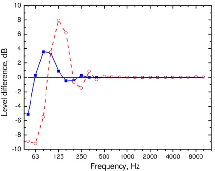
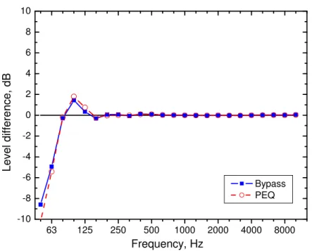
When instead a parametric equalizer was used to correct the loudspeaker response, the differences between time windowed results in an ordinary large room and those in an anechoic room were much smaller as shown in Figure 14. The largest differences are below the range of frequencies included in the calculated speech privacy measures. The parametric equalizer leads to essentially the same results as when the equalizer is

bypassed. Therefore the observed low frequency effects are due to the time windowing of the measured impulse response that is required to eliminate unwanted reflections. This is not surprising because the 5 ms window is quite short compared to the period of the signal at the lower frequencies. However, the 5 ms time window was selected as a suitable compromise that only causes significant problems below the frequency range of interest for speech privacy measurements.

(21)

63 125 250 500 1000 2000 4000 8000 -10 -8 -6 -4 -2 0 2 4 6 8 10 Bypass PEQ Leve l di fferen ce, dB Frequency, Hz

Figure 14. Differences between SPMSoft source levels measured by time windowing responses in an ordinary large room and those obtained in an anechoic room using a parametric equalizer (PEQ) and also with the equalizer bypassed.

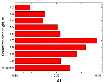
The time windowed measurements in the ordinary large room were made with the source and receiver 1 m apart and at least 2 m from all room surfaces. This was intended to be large enough to prevent unwanted reflections arriving within the 5 ms time window that was used. A further series of measurements was carried out to determine the effects of gradually introducing unwanted reflected sound by systematically lowering the source and receiver so that they gradually became closer to the floor. The height of the source and receiver were reduced from 2.0 m to 1.2 m in 0.1 m steps.

The effects of gradually adding an unwanted floor reflection will vary with frequency in a complex manner that will change with the actual height of the source and receiver. To evaluate the importance of the effects, the measured source levels were used to

recalculate AI values for an open-plan office workstation example. The resulting variations in the AI values for the varied source levels with effects of a floor reflection included are shown in Figure 15. Good agreement depends on carefully orienting the loudspeaker to point directly at the source for all cases. Figure 15 shows that for heights of 2.0 and 1.9 m, differences of ±0.01 in AI values are found. At lower heights larger differences occur. Using a 2.0 m height is adequate to eliminate floor reflection problems and source level measurements should be made with the source and receiver at least 2 m from all reflecting surfaces if an anechoic room is not available.

(22)

Anechoic 2.0 1.9 1.8 1.7 1.6 1.5 1.4 1.3 1.2 0.38 0.39 0.40 AI Sourc e /r ec eiv e r hei ght , m

Figure 15. Effect of gradually increased floor reflection on measured SPMSoft source levels (by varying the height of the source and receiver), illustrated by using the measured source levels to recalculate AI values for a pair of adjacent workstations using the varied source levels.

(23)

5. Repeatability of Measurements

The differences that are found when measurements are repeated are an indication of the reliability of the measurement. Several series of tests were carried out to evaluate how repeatable the speech privacy measurements are.

(a) Differences on exactly repeating measurements

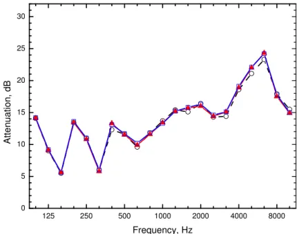
An example of the results of 3 re-measured sets of attenuation versus frequency data for the same situation are compared in Figure 16. All 3 measurements provided very similar results and the differences are mostly related to how carefully the exact source and receiver positions are repeated. Over the speech frequencies (160 to 5k Hz), the average of the absolute value of the differences in each 1/3-octave band was 0.35 dB. The differences in each 1/3-octave band varied from 0.0 to 1.0 dB.

125 250 500 1000 2000 4000 8000 0 5 10 15 20 25 30 Atte nua ti on, dB Frequency, Hz

Figure 16. Comparison of the results of three repeats of measured attenuation versus frequency between two adjacent workstations.

Over a series of 15 measurements (3 repeats of 5 conditions), the average of the absolute value of the differences in AI values was 0.0079 with a standard deviation of ±0.0041. The distribution of differences in AI values for the same 15 comparisons is shown in Figure 17. The average difference in AI values for these measurements was 0.0075 (shown by the vertical dashed line) with a standard deviation of 0.0049. AI values are normally only given to a resolution of 0.01. Since only 20% of the differences in Figure 17 were greater than 0.01, then most of the observed differences on repeating these measurements are usually no larger than the normal resolution of the AI measure.

(24)

-0.005 0.000 0.005 0.010 0.015 0.020 0 1 2 3 4 5 Fr equency of occur ance difference in AI

Figure 17. Distribution of differences in AI values for 15 repeated measurements. Vertical dashed line is mean difference, AI=0.0075.

(b) Differences related to small errors in repositioning source and receiver

To better understand the precision required in re-positioning the source and receiver, the effects of small systematic variations in their positions were evaluated. Three different sets of variations were measured. In the first set of variations the microphone was moved to 5 positions 5 cm from the original position. In the second set of variations the

microphone was moved to 5 positions 1 cm from the original position. In the third set of variations the loudspeaker was moved to positions 1 cm from the original position. In each case the variations also included one repeat of the original position. Table 1

summarises the results in terms of the standard deviations of the measured values over all variations of the positions.

AI SII STI Atten (A) Atten(avg)

Move Mic 5 cm 0.0033 0.0039 0.0088 0.11 0.14

Move Mic 1 cm 0.0044 0.0037 0.0019 0.11 0.10

Move loudspeaker 1 cm 0.0015 0.0013 0.0012 0.05 0.04

Table 3. Standard deviations of measured quantities for repeated measurements with small systematic variations of the microphone or receiver position. (AI Articulation Index, SII Speech Intelligibility Index, STI, Speech Transmission Index, Atten(A) A-weighted overall attenuation, dB, Atten(avg), attenuation arithmetically averaged over the speech frequencies 160 to 5k Hz, dB.

For AI, SII and attenuation measurements, moving the microphone by 5 cm had about the same effect as moving it 1 cm. Only for STI values did the larger movement have a clearly larger effect. However, moving the microphone 1 cm always had a larger effect than moving the loudspeaker 1 cm. That is, it is a little more important to re-position the microphone accurately than the loudspeaker. However, in all cases the differences, as indicated by the standard deviations in Table 3, are all very small. For example,

variations in AI values are almost always less than 0.01, the minimum resolution for this quantity. For the attenuations averaged over frequency, the standard deviations are small fractions of a decibel.

(25)

(c) Differences related to using different loudspeakers

One might expect to get similar results if similar loudspeakers are used. Measurements were made with 4 different loudspeakers. These are described in Table 2. While the B&K loudspeaker was close to ideally omni-directional, the others tended to approximate the directionality of a human talker. The PSB loudspeaker included two drivers.

Name Description

JSS Electro-Voice type 405-8H driver in an un-vented box with external dimensions 18.5 by 18.5 by 14.5 cm

NTI TalkBox

Small speech source with amplifier and using single loudspeaker driver B&K Bruel and Kjaer type 4295 omni-directional source

PSB PSB model Alpha Mite miniature bookshelf loudspeaker with two drivers

Table 4. Descriptions of 4 loudspeakers used in comparisons.

Figure 18 compares the measured attenuations for exactly the same conditions obtained using the 4 different loudspeakers. While the low frequency attenuations tend to be very similar, differences increase in magnitude with increasing frequency. The

omni-directional B&K loudspeaker is perhaps most different and is different over a broader range of frequencies. It is clear that it is not appropriate to suggest that the other loudspeakers are even approximately omni-directional. They are directional and their directionalities are all different. For example, the JSS loudspeaker has a characteristic peak in the attenuations at 5 and 6.3 kHz. This is due to the more directional

characteristics at these frequencies not radiating as much energy towards the ceiling, which leads to, increased attenuation values. Presumably the NTI source is also more directional at 8 and 10k Hz. Using the omni-directional B&K source tends to produce the lowest attenuations because it radiates more sound energy towards the ceiling. Since the main ceiling reflection often conveys the most energy to the receiver, the amount of sound energy directed towards the ceiling can have a large effect on the resulting attenuations.

Table 5 shows the AI values calculated for 9 different measurement positions with each of the 4 loudspeakers. The right hand side of the table shows the differences relative to the values obtained using the JSS loudspeaker (which was used for all other

measurements in this report). Using the different loudspeakers, the AI values varied from –0.071 to +0.078 or a range of 0.149 relative to the values obtained using the JSS source. Using the omni-directional B&K source would lead to AI values that were on average 0.06 smaller than those for the JSS loudspeaker.

These results suggest that one must be very careful when comparing results obtained using different loudspeakers. The possible differences due to using different loudspeakers are quite large and are much larger than the likely errors on repositioning the source and are subjectively important.

(26)

125 250 500 1000 2000 4000 8000 0 5 10 15 20 25 30 Attenu atio n, dB Frequency, Hz JSS NTI B&K PSB

Figure 18 Comparison of attenuations measured between two adjacent workstations for exactly the same conditions.

Mean AI Values from 9 measurements Differences re JSS loudspeaker results

JSS NTI B&K PSB JSS NTI B&K PSB

S1 R1 0.271 0.246 0.342 0.280 0.00 0.026 -0.071 -0.009 S1 R2 0.272 0.253 0.327 0.279 0.00 0.019 -0.055 -0.007 S1 R3 0.260 0.198 0.329 0.278 0.00 0.062 -0.069 -0.018 S2 R1 0.258 0.180 0.302 0.263 0.00 0.078 -0.044 -0.005 S2 R2 0.266 0.249 0.325 0.262 0.00 0.018 -0.059 0.004 S2 R3 0.273 0.257 0.335 0.272 0.00 0.016 -0.063 0.001 S3 R1 0.253 0.224 0.318 0.262 0.00 0.030 -0.065 -0.009 S3 R2 0.256 0.240 0.316 0.263 0.00 0.016 -0.061 -0.008 S3 R3 0.250 0.240 0.302 0.255 0.00 0.010 -0.052 -0.005 MAX 0.078 -0.044 0.004 MIN 0.010 -0.071 -0.018 AVG 0.030 -0.060 -0.006

Table 5. AI values measured for 9 different conditions between adjacent

workstations using 4 different loudspeakers. Right hand side of table indicates the differences in AI values relative to the AI values obtained when using the JSS loudspeaker.

(27)

6. Interpretation of Impulse Responses

As illustrated in Figure 1, SPMSoft displays the envelope of the initial portion of the measured impulse response describing the details of sound transmission between the source in one workstation and the receiver in another. Even the envelope of the measured Impulse Response (IR) can be quite complex and difficult to interpret. The diagnostic functions of SPMSoft calculate the expected arrival times of the two most important features of the IR for propagation between two adjacent rectangular workstations. These two features are: (a) the sound arriving by diffraction around the top of the separating panel and (b) the sound arriving via the initial ceiling reflection. SPMSoft calculates the arrival times of these two key events from the geometrical details that the user enters for the diagnostic calculations. The calculated arrival times are used to draw the red and blue boxes on the IR plot illustrated in Figure 1.

The peaks in the envelope of the IR within each box and the heights of the two boxes give some indication of the relative importance of these two key events. The heights of the actual response peaks are a more reliable indication than the heights of the boxes, which are influenced by possible errors in the estimated time of arrival of the two key events. If the energy arriving within the blue box is largest, then it is most important to reduce the energy diffracted around the top of the workstation panel. For example, the amplitude of this initial arrival could be reduced by using a higher panel. On the other hand if the energy within the red box is largest, it could be reduced by increasing the sound absorbing properties of the ceiling. It is important that the more serious of the two problems be first included in any attempt to improve speech privacy.

To illustrate the interpretation of these two key features of the envelope of the IR, Figure 19 shows 9 examples of IR envelope plots for systematically varied panel height and ceiling absorption. These were obtained from measurements of mock-up workstations with systematically varied panel height and ceiling absorption. The panel heights varied from 1.22 m (4 ft), to 1.52 m (5 ft) and 1.83 m (6ft), going from top to bottom on Figure 19. The Sound Absorption Average (SAA) of the ceilings varied from 0.57 to 0.97 and 1.08 as measured in a standard reverberation chamber test (ASTM C423). Each of the 9 IR envelope plots in this figure also includes the calculated AI value obtained using the same optimum masking noise spectrum in all cases. The AI values give an indication of the relative importance of the changes among the 9 different cases.

The blue arrows above the first peak of the 9 IR envelope plots indicate the sound energy arriving by diffracting around the top of the separating workstation panel. It is seen that in moving from left to right on Figure 19, the height of this initial peak stays more or less constant because it is related to the panel height, which is constant when moving from side to side on this graph. However, in moving from the top row to the bottom row the height of this peak decreases by approximately 16 dB as the panel height increases. The second (red) arrow indicates the peak associated with the sound energy arriving by way of the initial ceiling reflection. This second identified peak decreases significantly in going from left to right of Figure 19 as the average ceiling absorption (SAA) increases. To improve speech privacy and hence reduce AI values, one must first reduce the higher of these two peaks. Of course, when the two are almost equal both must be reduced to achieve a successful improvement in speech privacy.

(28)

40 45 50 55 60 65 Ceiling SAA = 0.57 Panel height = 1.22m AI = 0.39 D-C = 3.9 dB Le v e l, d B Ceiling SAA = 0.87 Panel height = 1.22m AI = 0.37 D-C = 3.6 dB Ceiling SAA = 1.08 Panel height = 1.22m AI = 0.36 D-C = 8.0 dB 40 45 50 55 60 65 Ceiling SAA = 0.57 Panel height = 1.52m AI = 0.29 D-C = -5.2 dB Le vel , dB Ceiling SAA = 0.87 Panel height = 1.52m AI = 0.26 D-C = -4.2 dB Ceiling SAA = 1.08 Panel height = 1.52m AI = 0.21 D-C = -0.5 dB 0 10 20 30 40 50 60 70 35 40 45 50 55 60 65 Ceiling SAA = 0.57 Panel height = 1.83m AI = 0.26 D-C = -11.3 dB Lev el , dB Time, ms 0 10 20 30 40 50 60 70 Ceiling SAA = 0.87 Panel height = 1.83m AI = 0.21 D-C = -10.6 dB Ceiling SAA = 1.08 Panel height = 1.83m AI = 0.14 D-C = - 6.9 dB Time, ms 0 10 20 30 40 50 60 70 Time, ms

Figure 19. Example impulse response envelope plots for varied ceiling absorption (increasing from left to right) and increasing panel height (increasing from top to bottom)

(29)

The displayed IR envelope plot can also indicate other significant strong peaks that occur such as when a pair of adjacent workstations is next to windows. There is often a gap between the workstation panels and the windows allowing strong reflections off the windows into the adjacent workstation. Figure 20 illustrates a measured IR envelope with a significant window reflection. Any unusually strong peak indicates an event that may contribute to significantly reducing speech privacy and should be investigated.

10 20 30 40 50 0 50 60 70 Level, dB 10 20 30 40 Time, ms

Figure 20. Measured impulse response envelope with a significant reflection from adjacent windows indicated by the red arrow.

Impulse Response Screen Ceiling

Even when there are no unusually strong peaks, there can be significant differences between measured IR plots. Figure 21 compares IR envelope plots measured in two different offices. In the lower plot the level of reflections arriving after the two initial events is much higher than in the upper plot. The data for the lower plot was from an office with more reflective surfaces than the other.

(30)

10 20 30 40 50 0 10 20 30 40 50 60 7 Time, ms Level, dB 0

Figure 21. Comparison of measurements between adjacent workstations in two different offices. The upper IR envelope plot was from an office with relatively high workstation panels and highly absorbing workstation panels and ceiling. The lower IR envelope plot was from an office, which again had relatively high

workstation panels but had a highly reflective ceiling. In both cases the initial sound diffracted over the separating panel (in the blue box) is not the highest peak because of the high workstation panels. However, in the lower plot, the ceiling reflection (red box) is higher and the amplitudes of the many following reflections are much higher than in the upper IR envelope plot.

(31)

7. Spatial Variations within Workstations

Sound propagation from one workstation to another is quite complex and to more completely understand the details of each situation multiple measurements may be necessary. To illustrate what is possible, Figure 22 shows the results of measurements from one workstation (#4 with the source at the location of the red star) to two adjacent workstations (#3 and #5). Measurements in the two receiving workstations were made at 0.3 m intervals and contour plots were fitted to the results. The contours are drawn at 0.05 intervals of AI values. 2.14 m 2.77 m 4.28 m 5.54 m 1.68 m 1.11 m 4 3 ₂ 5 0.15 0.20 0.25 0.30 0.35 0.40 0.45 0.50 0.55

*

Figure 22. Contour plots fitted to measured AI values. The source was located at the red star in workstation #4. Contours are at intervals of 0.05 in AI values.

As one would expect, when moving away from the source, the contour plots indicate increasing AI values because locations closer to the separating panels have less diffracted sound energy. In optical terms, they are deeper into the shadow of the panels. For

locations more distant from the separating panels, AI values will be more dependent on the effects of various reflections. Because there are no panels at the upper side of

workstations 4 and 5 in Figure 22, strong reflections from the wall (not shown but at the top of the figure) lead to higher AI values in workstation 5 than in workstation 3. Except for locations close to the separating panels, AI values vary relatively gradually and there is usually no need for such large numbers of measurements as included in Figure 22. Quite often a single measurement from the centre of one workstation to the centre of a neighbouring workstation is adequate to determine if there are serious

(32)

problems. A few more measurements may be necessary to fully understand situations where more serious problems are found.

(33)

8. Optimising Measurements

The various speech privacy measures are calculated from the expected speech levels at the receiver position and the ambient noise levels at that position. Measuring the ambient noise levels is straightforward but calculating the expected speech levels at the receiver position requires an accurate measurement of sound attenuation between the source and receiver position. Using conventional measurements, the test signal would have to be loud enough at the receiver position to be well above the background noise level. When using an impulse response to measure the attenuation, the test signal should also be at a reasonably high sound level. However, repeated measurements can also be averaged to increase the effective level of the received test signal relative to the ambient noise. Sometimes using a lower level test signal combined with signal averaging can make the measurements less disturbing to office occupants. Averaging can also make it possible to measure over larger distances, for which greater attenuations would occur in offices.

(a) The combined effects of signal level, ambient noise level and number of averages

Systematic measurements between a pair of workstations were made to illustrate the benefits of various combinations of test signal level and numbers of averages. Three different output signal levels were used which are referred to as –20, -30 and –40 dB. These are decibels relative to the maximum possible output of the 16 bit sound card and for these results correspond approximately to maximum overall levels of 60, 50, and 40 dB(A) at 1 m in a free field for the amplifier and loudspeaker used. Ambient noise with an approximately neutral spectrum shape (-5 dB/octave) was created electronically. Noise levels were varied from 25 to 55 dBA.

25 30 35 40 45 50 55 0.0 0.1 0.2 0.3 0.4 0.5 0.6 0.7 0.8 0.9 AI BG, dBA 1 repeat 3 repeats 6 repeats 12 repeats 24 repeats -15 dB

Figure 23. Measured AI value versus A-weighted background noise level (BG, dBA) for various numbers of repeats with a –20 dB output signal level and compared with the reference case using 24 averages and an output signal level of –15 dB.

Figure 23 shows results for a -20 dB output test signal level. In this and the next few figures, the results are compared with a reference case of 24 repeats and an output signal level of –15 dB which was found to give near perfect results for these measurement conditions. In Figure 23 the output signal level (-20 dB) was quite high and only a small number of repeats (6 or 12) leads to close agreement with the reference case for even the

(34)

highest included ambient noise level (55 dBA). In a noisy office using 12 repeats and an output level of –20 dB would provide accurate results. In a quieter office fewer repeats could be used.

Figure 24 shows similar results with a reduced output signal level of –30 dB. In this case an increased number of averages is more often necessary. Even with background noise levels as low as 40 dBA, when using this test signal level some averaging of repeated signals is beneficial. At the highest background level included here (55 dBA) and this test signal level, 24 repeats are required to get really accurate AI values.

25 30 35 40 45 50 55 0.0 0.1 0.2 0.3 0.4 0.5 0.6 0.7 0.8 0.9 1 repeat 3 repeats 6 repeats 12 repeats 24 repeats 48 repeats 96 repeats 24 repeats -15 dB AI BG, dBA

Figure 24. Measured AI value versus A-weighted background noise level (BG, dBA) for various numbers of repeats with a –30 dB output signal level and compared with the reference case of 24 averages and -15 dB signal level.

The results using the –40 dB output signal level are shown in Figure 25. For this very low test signal level, some averaging is required at all ambient noise levels included in these tests (25 to 55 dBA). At the highest ambient noise levels (50 and 55 dBA), even 96 averages were not enough to get close agreement with the reference case. In very noisy offices it would be necessary to use a higher test signal level than –40 dB.

By comparing the results in these figures, one sees that increasing the test signal by 10 dB is approximately equivalent to using 10 times as many averages. However, a large number of averages can be quite time consuming. For example, a measurement using 96 averages takes about 10 minutes. In most cases it would be more effective to increase the test signal level. If the maximum acceptable test signal level is reached or if the test signal is disturbing occupants, then using an increased number of averages can make it possible to obtain accurate results with a lower test signal level. Figures 23 to 25 can be used to estimate the likely number of averages required for a particular situation.

(35)

25 30 35 40 45 50 55 0.0 0.1 0.2 0.3 0.4 0.5 0.6 0.7 0.8 0.9 1 repeat 3 repeats 6 repeats 12 repeats 24 repeats 48 repeats 96 repeats 24 repeats -15 dB AI BG, dBA

Figure 25. Measured AI value versus A-weighted background noise level (BG, dBA) for various numbers of repeats with a –40 dB output signal level and compared with the reference case of 24 averages and -15 dB signal level.

25 30 35 40 45 50 55 0.0 0.1 0.2 0.3 0.4 0.5 0.6 0.7 0.8 0.9 1 repeat 3 repeats 6 repeats 12 repeats 24 repeats 48 repeats 96 repeats 24 repeats -15 dB SI I BG, dBA

Figure 26. Measured SII value versus A-weighted background noise level (BG, dBA) for various numbers of repeats with a –40 dB output signal level and compared with the reference case of 24 averages and -15 dB signal level.

Similar results were obtained for plots of SII values versus background noise levels for various numbers of repeats. Figure 26 plots measured SII values versus ambient noise level for the case of a –40 dB output signal level. The results are similar to those in Figure 25 for AI values and the same output signal level except that SII values are a little

(36)

larger than the corresponding AI values. However, for most ambient noise levels a number of repeats are required for good agreement with the reference case.

Figure 27 shows the effects of varied numbers of averages on STI values for the same range of background noise levels and the same –40 dB output signal level as used to obtain the results in Figures 25 and 26. Again a larger number of averages leads to closer agreement with the reference case but the pattern of results is quite different for STI values. AI and SII measurements depend on an accurate simple attenuation measurement. STI is much more complex and requires more of the impulse response to be correctly measured and hence usually requires more averages to get close agreement with the reference case. 25 30 35 40 45 50 55 0.0 0.1 0.2 0.3 0.4 0.5 0.6 0.7 0.8 0.9 1 repeat 3 repeats 6 repeats 12 repeats 24 repeats 48 repeats 96 repeats 24 repeats -15 dB STI BG, dBA

Figure 27. Measured STI value versus A-weighted background noise level (BG, dBA) for various numbers of repeats with a –40 dB output signal level and compared with the reference case of 24 averages and -15 dB signal level

(37)

125 250 500 1000 2000 4000 8000 -25 -20 -15 -10 -5 0 5 10 15 20 25 30 Att en uatio n, dB Frequency, Hz 1 lrepeat 3 repeats 6 repeats 12 repeats 24 repeats 48 lrepeats 96 repeats 24 repeats -15 dB

Figure 28. Measured 1/3-octave band attenuations for an output signal level of – 40 dB and an ambient noise level of 46 dBA for varied number of averages and compared with the reference case using 24 averages and an output signal level of -15 dB.

Examining the accuracy of measurements in terms of AI values or values of the other speech privacy measures gives a good overview of the combined effects of signal level and number of averages for various combinations of conditions. However, examining the effects of signal level and number of averages on the actual attenuation measurements shows in more detail how the measured attenuations gradually improve as the number of averages is increased. Figure 28 plots measured attenuations for a –40 dB output signal level and a 46 dBA ambient noise level to illustrate how the measured attenuation values gradually approach the reference case values as the number of averages is increased. In this example, even 96 repeats does not lead to complete agreement with the reference case at all frequencies. Better agreement can be obtained using a higher output test signal level.

One can also examine the benefits of increased numbers of averages by looking at IR envelope plots. When the test signal level is not high enough or there are not a large enough number of averages, the IR envelope plot will be contaminated with noise. Often the noise will be most visible during the initial time period before the arrival of the first test sound. Figure 29 shows a plot of the reference case IR envelope plot corresponding to an output test signal level of –15 dB and 24 averages.

(38)

10 20 30 40 50 0 10 20 30 40 50 60 7 Time, ms Level, dB 0

Figure 29. Impulse response envelope plot for reference case of –15 dB output signal level and 24 averages.

Figure 30 plots the IR envelop for the same source and receiver locations but with a signal level of -30 dB and only 1 repeat. This IR envelope plot is quite noisy compared to the reference condition in Figure 29. When more averages are used, the result shown in Figure 31 was obtained. Figure 31 is the IR envelope plot for a signal level of –30 dB and 24 averages. The IR envelope plot in Figure 31 is much less contaminated with noise and looks quite similar to the reference case in Figure 29. The AI for the reference case was 0.29. The AI values for Figures 30 and 31 were 0.39 and 0.29 respectively. That is, by increasing the number of averages, the AI value agrees well with that of the reference case. 10 20 30 40 50 0 10 20 30 40 50 60 7 Time, ms Level, dB 0

Figure 30. Same condition as Figure 29 measured with a much lower signal level (-30 dB) and only 1 repeat.

(39)

10 20 30 40 50 0 10 20 30 40 50 60 Time, ms Level, dB 70

Figure 31. Same condition as Figure 29 measured with a much lower signal level (-30 dB) and 24 averages.

(b) Selecting a suitable combination of signal level and number of averages

Figures 23, 24 and 25 can be used to calculate the errors in measured AI values as the differences between the measured values for each combination of signal level, ambient noise level and number of repeats with the AI value for the corresponding reference case. Figure 32 shows the errors in AI values for the case of a signal level of –20 dB plotted versus ambient noise level for each of the different numbers of averages. We can say that an accurate measurement is one that is within ±0.01 of the correct value, which is the smallest change in AI values which are defined to only 2 decimal places.

For the results in Figure 32, using even 3 averages results in errors in AI values slightly less than 0.01for noise levels up to 46 dBA. By increasing the number of averages to 12 the errors in AI values would be less than 0.01 for all noise levels. In most case the errors would be much less than 0.01.

Figure 33 similarly plots the errors in AI values for a test signal level reduced to –30 dB. At this reduced test signal level more repeats are needed for the measured values to agree within 0.01 with the reference values as the noise levels increase. Using 12 repeats, as in the previous example, is only satisfactory up to an ambient noise level of 39 dBA. To get an accurate result at the highest noise level (55 dBA) at least 48 averages are required.

(40)

25 30 35 40 45 50 55 0.0 0.1 0.2 0.3 0.4 0.5 0.6 E rro r i n AI BG, dBA 1 repeat 3 repeats 6 repeats 12 repeats 24 repeats 48 repeats 96 repeats

Figure 32. Plot of Errors in AI versus background noise levels (BG, dBA) for varied numbers of repeats and a test signal level of -20 dB.

25 30 35 40 45 50 55 0.0 0.1 0.2 0.3 0.4 0.5 0.6 Err o r in AI BG, dBA 1 repeat 3 repeats 6 repeats 12 repeats 24 repeats 48 repeats 96 repeats

Figure 33. Plot of Errors in AI versus background noise levels (BG, dBA) for varied numbers of repeats and a test signal level of –30 dB.

(41)

25 30 35 40 45 50 55 0.0 0.1 0.2 0.3 0.4 0.5 0.6 Err o r in AI BG, dBA 1 repeat 3 repeats 6 repeats 12 repeats 24 repeats 48 repeats 96 repeats

Figure 34. Plot of Errors in AI versus background noise levels (BG, dBA) for varied numbers of repeats and a test signal level of –40 dB.

Figure 34 shows the errors in AI values for a test signal level of –40 dB. For such a low test signal level it is difficult to get accurate AI values except for quite low ambient noise levels. Using 12 repeats would provide accurate results up to an ambient noise level of 31 dBA and using 96 repeats would provide accurate AI values for ambient noise levels up to 46 dBA.

Similar error plots can be obtained in terms of SII values but lead to the same conclusions as to the required signal level and number of averages for an accurate result. To illustrate this Figure 35 plots errors in SII values for a test signal level of –40 dB. As in Figure 34 for errors in AI values, 12 repeats would provide accurate results up to an ambient noise level of 31 dBA but 96 repeats would be required for accurate SII values for ambient noise levels up to 46 dBA.

(42)

. 25 30 35 40 45 50 55 0.0 0.1 0.2 0.3 0.4 0.5 0.6 Err o r in SI I BG, dBA 1 repeat 3 repeats 6 repeats 12 repeats 24 repeats 48 repeats 96 repeats

Figure 35. Plot of Errors in SII versus background noise levels (BG, dBA) for varied numbers of repeats and a test signal level of –40 dB.

25 30 35 40 45 50 55 -0.3 -0.2 -0.1 0.0 Error i n ST I BG, dBA 1 repeat 24 repeats 3 repeats 48 repeats 6 repeats 96 repeats 12 repeats

Figure 36. Plot of Errors in STI versus background noise levels (BG, dBA) for varied numbers of repeats and a test signal level of –40 dB.

The error plots of STI values are quite different than those for AI and SII values. Figure 36 shows the errors for STI values for the same –40 dB signal level as the previous two plots. Almost none of the results lead to an accurate STI value and the errors in STI are much bigger than those for AI and SII for the corresponding conditions. Accurate STI measurements would require higher output signal levels than –40 dB.

(43)

(c) Effects of occupants

One of the benefits of using impulse response measurements is that accurate attenuation measurements between workstations can be made with relatively low level test sounds. This makes it possible to measure speech privacy in occupied offices during normal working hours. This was initially confirmed by making systematic measurements with interfering speech sounds, which were compared with the same ideal reference case results used in previous comparisons. Interfering speech was produced by playing recorded speech into an adjacent workstation while measuring speech privacy. That is, speech privacy was measured between workstation A and B while interfering speech was produced in workstation C adjacent to the receiving workstation B. The speech was played back with a level of 56 dBA measured at 1 m in a free field. This is about 5 dB higher in level than average speech levels found in open-plan offices [11], and hence represents a louder than normal but not too unusual speech interference.

The new measurements followed the procedures of those in the previous section. Speech privacy was measured between a pair of adjacent workstations with varied levels of ambient noise. Ambient noise was again electronically generated with a neutral spectrum shape decreasing with increasing frequency at a rate of -5 dB per octave. Overall noise levels varied from 41 to 52 dBA.

25 30 35 40 45 50 55 0.0 0.1 0.2 0.3 0.4 0.5 0.6 0.7 0.8 0.9 AI BG, dBA 1 repeat 3 repeats 6 repeats 12 repeats 24 repeats Reference

Figure 37. Measured AI values in the presence of interfering speech plotted versus A-weighted background noise level (BG, dBA) for varied number of averages with a –20 dB output signal level and compared with the reference case using 24 averages and an output signal level of -15 dB.

Figure 37 plots measured AI values versus ambient noise level for varied number of averages and an output signal level of –20 dB. For this relatively high signal level, the interfering speech had very little effect. Only for the case of 1 average and the highest ambient noise level did the measured AI values deviate significantly from the reference case value. This deviation is similar to that in Figure 23 without interfering speech and simply indicates an inadequate number of averages to obtain an accurate attenuation

(44)

measurement with this level of ambient noise. There is no evidence of any influence by the interfering speech sound.

The effects of interfering speech with a reduced test signal level of –30 dB are shown in Figure 38. In this figure there are large deviations from the reference case. However. The results in Figure 38 are very similar to those in Figure 24, which was obtained for the same conditions but without any interfering speech sounds. When Figure 24 and 38 are compared in detail there is again no evidence of a significant effect of the interfering speech sounds on the measured AI values. These tests indicate that speech privacy measurements can be accurately carried out in the presence of moderate levels of interfering speech sounds.

25 30 35 40 45 50 55 0.0 0.1 0.2 0.3 0.4 0.5 0.6 0.7 0.8 0.9 AI BG, dBA 1 repeat 3 repeats 6 repeats 12 repeats 24 repeats Reference

Figure 38. Measured AI value with interfering speech versus A-weighted

background noise level (BG, dBA) for various numbers of repeats with a –30 dB output signal level and compared with the reference case using 24 averages and an output signal level of -15 dB.