Biomimetic improvement of the maneuvering qualities of unmanned underwater vehicles

Biomimetic Improvement of the Maneuvering Qualities of

Unmanned Underwater Vehicles

By Yuri Trakht

M.Sc., Mechanical Engineering

Technion - Israel Institute of Technology, 2013

SUBMITTED TO THE DEPARTMENTS OF MECHANICAL ENGINEERING IN PARTIAL FULFILLMENT OF THE REQUIREMENTS FOR THE DEGREE OF

MASTER OF SCIENCE IN NAVAL ARCHITECTURE AND MARINE ENGINEERING AND

MASTER OF SCIENCE IN MECHANICAL ENGINEERING AT THE

MASSACHUSETTS INSTITUTE OF TECHNOLOGY

February 2019

0 2019 Massachusetts Institute of Technology. All rights reserved. The author hereby grants to MIT permission to reproduce

and to distribute publicly paper and electronic copies of this thesis document in whole or in part In any medium now known or hereafter created.

Signature redacted

Signature of Author:

D'eartment of Mechanical Engineering January 18, 2019

Signature redacted

Certified by: ________ _{_________}

Michael Triantafyllou The Henry L. a r -.

Dherty

Signature

redacted

Accepted by:

Nicolas Hadjiconstantinou

FT HChairman, Committee on Graduate Students

Biomimetic Improvement of the Maneuvering Qualities of

Unmanned Underwater Vehicles

By Yuri Trakht

M.Sc., Mechanical Engineering

Technion - Israel Institute of Technology, 2013

Submitted to the Department of Mechanical Engineering

on 1 8th January 2019, in Partial Fulfillment of the requirements for the Degrees of

Master of Science in Naval Architecture and Marine Engineering

and

Master of Science in Mechanical Engineering

Abstract

In recent years, biomimetics has been used as a source of inspiration to improve the performance of engineered systems in several disciplines. In this thesis, we emulate the function of the retractable dorsal fins in tunas to improve the maneuvering performance of a typical autonomous underwater vehicle, the REMUS 100 AUV. We are introducing dorsal-like fins on the AUV that can be erected to alter its maneuvering hydrodynamic coefficients, and hence affect the transient and steady-state turning response.

In order to study systematically the effect of adding dorsal fins, we built a six degrees of freedom simulation model of the REMUS AUV. The model included body and rudder lift forces and moments, added mass forces and moments, gyroscopic and centrifugal forces, drag forces and moments, and body forces and moments such as buoyancy and gravity terms. To target the horizontal plane maneuvering characteristics, we reduced the model to a 3 DOF simulation, allowing the dorsal fin to vary in area, location along the length of the AUV, as well as having a turning angle with respect to the REMUS x-axis.

We find that the addition of the fin can improve the performance, as measured by the radius of turning and rate of turning, moderately only when placed ahead of the center of gravity. However, when the dorsal fin is also allowed to rotate in the opposite direction that the rudder, substantial improvement in maneuvering performance is noted, increasing the turning rate up to 25%.

Thesis supervisor: Michael Triantafyllou

Acknowledgment

First, I would like to thank my Thesis supervisor, Professor Michael Triantafyllou, the head of The MIT Sea Grant who guided, motivated and encouraged me to work on this research. Michael, with profound knowledge and generous patience, helped me and guided me step by step to reach this final goal. Next, I would like to thank Nastasia Winey who helped and guided me with her study, so I could join and contribute to her research.

I would like to thank the Israeli Navy for sponsoring my family and me during my studies at MIT. Most importantly, I would like to thank my family. First, to my wife Lilya, who was always there for me, encouraged me to set goals and pushed me to reach them. Thank you for your love, your support, your enormous patience and being my best friend. Second, I would like to thank my lovely daughter Sophie. Last, I would like to thank my parents, who without their push, I would not have even dreamed of submitting an MIT thesis.

Table of Contents

1 Introduction ... 11

2 REM U S Geom etry ... 12

3 Derivation of Equations of M otion ... 16

3.1 Kinematics and Coordinate System Definition ... 16

3.2 Newton's 2"d Law of M otion... 18

3.3 Forces Derivation...20

3.4 Added M ass M atrix...20

3.5 Added M ass Forces...23

3 .6 D rag F orces...2 7 3 .7 B o d y L ift...2 9 3.8 Fin Lift and Drag ... 31

3.9 Total Hydrodynamic Forces... 35

3.10 Hydrostatic and Gravity Forces...36

3.11 Propulsion Force...38

3.12 General Equations of M otion...38

4 N um erical Sim ulation ... 42

4.1 State Space Representation... 42

4.2 M aneuvering Simulation ... 42

4.3 Forces Evaluation ... 46

5 Additional Fin for M aneuvering Im provem ent ... 49

5.1 Additional Fin with Variable Angle ... 54

5.2 Transient M aneuvering Performances... 62

6 Sum m ary and Conclusion... 69

7 References ... 70

Appendix A - Results for Different Rudder and Fin Areas...71

List of Figures

Figure 1: R E M U S G eom etry -[3]...13

F igure 2: R E M U S F ins - [3]...13

Figure 3: Profile View -REMUS Hull and Fins... 14

Figure 4: REMUS, 3D view from MATLAB...14

F igure 5: F in H eight A bove H ull...15

F igure 6: C oordinate System ... 16

Figure 7: Ellipsoidal Least Square Fitting of the REMUS Hull...22

Figure 8: Lift forces Applied on the Body ... 30

Figure 9: Fin Horizontal Velocity Diagram, Positive Rudder Angle. ... 32

Figure 10: Fin Horizontal Velocity Diagram, Negative Rudder Angle. ... 32

Figure 11: Circle maneuver for various rudder angles, X-Y plot. ... 43

Figure 12: Circle Maneuver for Various rudder angles, Yaw rate as a Function of Time...44

Figure 13: Circle Maneuver for Various Rudder Angles, Drift Angle as a Function of Time...44

Figure 14: Circle Maneuver for Various Rudder Angles, Surge Velocity as a Function of Time....44

Figure 15: Summary of All Maneuvering Parameters as a Function of Rudder Angle...45

Figure 16: Free-Body Diagram on the Vehicle During Turning. X, Y Plane...46

F igu re 17: X F orces. ... 4 7 F igu re 18 : Y F orces. ... 4 7 F igure 19: N M om ents...48

Figure 20: 4' R udder A ngle Forces... 48

Figure 21: 100 R udder A ngle Forces ... 48

Figure 22: REMUS with Additional Maneuvering Fin ... 49

Figure 23: Comparison of Tactical Radii in Turning... 50

Figure 24: Comparison of Yaw Rate in Turning...50

Figure 25: Comparison of Drift Angle in Turning. ... 50

Figure 27: Free-Body Diagram with Different Fin Locations, Rudder Angle 40, (A) - Without Fin,

(B) Location=0, (C) Location=0.1, (D) Location=0.3 ... 52

Figure 28: Free-Body Diagram with Different Fin Locations, Rudder Angle 10', (D) - Without Fin, (B) Location=0, (C) Location=0.1, (D) Location=0.3 ... ₅₃

Figure 29: Fin Angle Definition, Left - Positive Angle, Right - Negative Angle. ... 54

Figure 30: Turning Radius as a Function of Fin and Rudder Angles...55

Figure 31: Yaw Rate as a Function of Fin and Rudder Angles...56

Figure 32: Drift Angle as a Function of Fin and Rudder Angles...57

Figure 33: End Velocity as a Function of Fin and Rudder Angles...58

Figure 34: Turning Radius with Rudder of 10' and Fin of -10 . ... 60

Figure 35: Yaw Rate with Rudder of 100 and Fin of -10 ... 60

Figure 36: Drift Angle with Rudder of 10' and Fin of -10 . ... 61

Figure 37: End Velocity with Rudder of 10' and Fin of -10 ... 61

Figure 38: Transient Performances Definition... ₆₂

Figure 39: Transient Maneuvering Performances, Fin Location =-0.3. ... 63

Figure 40: Transient Maneuvering Performances, Fin Location =-0.. ... 63

Figure 41: Transient Maneuvering Performances, Fin Location =0.1. ... 65

Figure 42: Transient Maneuvering Performances, Fin Location =0.4. ... 66

Figure 43: Transient Performance Results, Rudder=+10, Fin=-100 , x=10 ... . . . . 67

Figure 44: Transient Performance Results, Rudder=+10, Fin=-100 , xy=20 ... . . . . 68

List of Tables

T able 1: N ose P aram eters...12

T able 2: T ail P aram eters ... 13

T able 3: D istance P aram eters...14

Table 4: Added Mass Generalized Forces Coefficients and their Evaluation...26

Table 5: Turning Results from Variation of Rudder and Fin Area Ratios Where the Fin Location is 0.15 M eters Forward of Center of Gravity. ... 71

1 Introduction

In the recent years, autonomous underwater vehicles have become very popular in the military and the commercial world. Thanks to high-resolution sonar systems, high definition underwater cameras, advanced navigation systems, and sophisticated machine learning techniques, the capabilities of such AUVs have increased dramatically, giving the Navy and the commercial world great benefits. A key parameter used to select an AUV is its maneuvering performance. Maneuvering performance based on a vehicle's navigation system, control system, and its hydrodynamic characteristics. Triantafyllou [1], suggested a biomimetic design of underwater vehicle using the concept of erectable fins to improve flexibility in high-speed transient motions. This concept mimics a tuna erecting its dorsal and anal fins when high maneuverability is needed. The effectiveness of erectable fins is highlighted by utilization of the lymphatic system as the hydraulic power for the erection mechanism [2]. Using this important system focused solely on erecting these fins emphasizes how vital these fins are to a tuna's survival.

This research focuses on applying this concept of the tuna's retractable dorsal fin to a well-known AUV, REMUS 100, designed by the Oceanographic Systems Laboratory (OSL) in the Woods Hole Oceanographic Institute. All the geometric properties for REMUS 100 taken from the work of Prestero [3].

A full 6 DOF model was built, to examine and investigate the effects of an additional fin on the maneuvering performance of REMUS. The model derived from the kinematic relationship and Newton's second law of motion. The Kirchhoff assumptions used to derive the added inertia and Munk moments of the system. Body lift forces which represent suction forces due to the separation of the boundary layer approximated using Hoerner's Lift book [4]. The rudders and stern plane lift forces treated using the 3D lifting surfaces theory approximation. Hydrostatic and gravity forces added with help of the coordinate transformation from the global coordinate system and the local body attached system. The thrust was assumed to be constant and, found by the force needed to stay at maximal constant speed, the propeller heeling torque was also added according to sea trial results. To analyze the models maneuvering performances, it degenerated to a 3 DOF maneuvering model by zeroing the vertical velocity, pitch rate, and initial heeling angle and heeling moment produced by the propeller to model horizontal-only turning effects.

2 REMUS Geometry

The REMUS geometry described as a revolved profile that constructed from 3 individual parts: nose,

tail and the mid-section.

The nose section profile is a revolved surface with radius r described by the following function:

x+ x + aoffset - a (1)

r(x) = - d

-

where x is the distance along the axis of revolution.

The following parameters describe the nose geometry:

Table 1: Nose Parameters

Variable Value d 0.191 a 0.191 aoffset 0.0165 n ₂ xo -0.2625 d 0.191

The following equation gives the tail profile:

1

r3d

r(x)= 1d- 3

[

where If represent the body length without the nose and is if = a + b - aoffset . Here x is the

distance along the axis of the revolution.

Table 2: Tail Parameters

Variable

Value

d

0.191

a

0.191

b

0.654

0.0165

6

0.436

Figure 1: REMUS Geometry

_~[3]

Coffset -c

~

b

Figure 2: REMUS Fins

[3]

6.9 cm 8.9cm 13.1 cm 3.3 cm 6.2 m-4m -.2.9 CM 0' a 5. 1. cm 14.2 5.mc

aOfSet

V

.

FA.

b

Distances table

Table 3: Distance Parameters

Variable Meaning Value (m)

Xb2

Tip of the vehicle nose

0.61

Xb

End of the nose section

0.437

Xt2

Start of the tail section

-0.218

Xf2

Start of the fin section

-0.578

Xf

End of the fin section

-0.668

Xt

End of the vehicle

-0.721

Figure 3: Profile View -REMUS Hull and Fins.

K'

_-0.6

_-0.4

_-0.2

₀

_0.2

_0.4

REMUS Fins

--

REMUS Hull

0.6

Figure 4: REMUS, 3D view from MATLAB.

0.1 0--0.1 - . -0.4 - . -00 2 _{0 0.1} 2 0.4 -0.1

X -

Axis

0.1

0

-0.1

Fin geometry calculation:

Integration of the fin height above the hull gives the fin area as shown in Figure 5.

Figure 5: Fin Height Above Hull

0.12 F 0.1 0.08 0.06 0.64 0.02 -0.68 -0.66 -0.64 -0.62 -0.6 -0.58 -0.56 -0.54 X -Axis

The integration gives fin area Sf jn of 0.0062m2, and a fin span of 0.0943m.

REMUS Fins

- _{REMUS Hull}

-3 Derivation of Equations of Motion

3.1 Kinematics and Coordinate System Definition

First, the coordinate system of the underwater vehicle is defined as in Figure 6. The location of a

fixed position in the underwater vehicle 00 in an inertial coordinate system, relatively to the earth, is

r = [x y z] ₍₃₎

where x is the surge direction, y is the sway direction toward starboard and z is the heave direction

downwards.

Figure 6: Coordinate System

Body-fibd ferna

z

The Euler angles, which represent the orientation of the underwater vehicle relative to the inertial

coordinate system are

= 6 ]T (4)

where q5 is the roll angle, 6 is the pitch angle and

4

where u is the surge velocity, v is the sway velocity and w is the heave velocity.

The vehicle angular velocity is

-=[P

where p is the roll rate, q is the pitch rate and r is the yaw rate.

The transformation between the local body-fixed coordinate system velocity VO = [U v w]T and

the global velocity r4 = [k j ] given by

=

[

where the transformation matrix is

-cos4 Icos 6

R1(6)= sinV)cose

-sin 6

- sin~ cos q5 + cos 0 sin 6 sin

45

cos 0 cos

4

The transformation from local angular rates Wi = [p q

sin ip sin P + cos 1/ cos

4

-- cos 4, sin

4

4)

cos6 cos

4

r]T to the Euler angle velocities

[4

4)

sin

4P

q5

cos

4

6--1

+-Summary of the transition of both the angle rates and the velocities in block form:

(8) (9) (10) O= -1 R2 (0)= 0 0

Si V z _{R1(0) 0}

]

3.2 Newton's

Law of Motion

Consider an underwater vehicle whose center of mass is at rG, its velocity is i30 and its angular velocity is W' in the body coordinate system. According to Newton's 2nd law, the total force applied

on the body is the total derivative of the mass times the velocity along the center of mass plus the velocity due to the rotation:

d

F =m -- (0 +v w (12)

Expanding the force gives a partial derivative of i3O with other angular velocity terms:

F =

Z(13)

(at

dt

Expansion of the Force vector into 3 scalar equations, and application of the port-starboard symmetry gives:

X =m[t + qw -rv - (q2 _+rz)XG

+ (rp + )ZG]

Y =m[7 - pw + ru + (qp + ) xG + (rq - P)ZG (14)

Z =m[w + pv - qu + (pr - )xG - (p q2 )ZG

where X, Y, Z are the forces, u, v, w are the surge sway and heave velocities and p, q, r are the roll pitch and yaw velocities. xg and Zg are the locations of the center of gravity from the origin.

setting x. to zero ,simplifies equations system (14) as:

X = m[t + qw - rv + (rp + q)ZG]

Y = m[ - pw +ru + (rq - P)ZG] (15)

Z = m[W + pv - qu - (p2

+ q2)ZG

Similarly, Newton's law for summed particle moments:

N

(Mi + r-i X Fi)

1=1 N N ( = x + + (x)io + miri x

L

(16)

where i represents each particle, its location and the forces and moments applying on him. The symmetry of the vehicle, inertia cross term ignored, and the vector equation above splits into 3 equations of motion for rotation:

K = Ixxp + (Izz - Iyy)rq - mZG (f + ru - pW)

M = Iyy4 + (Ixx - Izz)pr + m[ZG (t + qw - rv) - XG ( + pv - qu)] (17)

N = Izzt + (iyy - Ixx)pq + mxG (P + ru - pW)

where IXXIYY,'Izz are the mass moments of inertia about the x, y, z axis respectfully. Using information about the symmetry and the location of the center of gravity discussed earlier, (17) simplifies to

K = Ixxp + (Izz - Iyy)rq - mZG (f + ru - pW)

M = YY + (IXX - Izz)pr + mZG (t + qw - rv) (18)

3.3 Forces Derivation

The forces presented in the last chapter, represent the total external generalized forces applied to the correspondent generalized coordinate. These forces are divided into 3 main categories [5]: Water-induced forces such as added inertia forces (added mass), hydrodynamic damping, drag forces, and hydrostatic forces. The second category includes environmental forces such as wind, waves and ocean currents. The last category includes the propulsion and control surfaces forces such as propellers thrust and control surface lift forces. This work covers only the first and the last category forces.

3.4 Added Mass Matrix

The 6 DOF added mass matrix consists of 36 elements:

-a

a

a

s

At

XV

XVw

Xr%-yr

where Xg for example, is the hydrodynamic added mass force in the X direction due to acceleration

in the i direction.

From symmetry, the added mass matrix reduces to the following structure (Ai1 = Aji)

-a

a

s

Xi

ZIAI

Xp

X4

Y4

ZO

reducing the number of coefficients from 36 to

plane and X-Y plane, the matrix reduces to:

-all 0 0 0 0 0 -Xu 0 0 0 0

0-0

0

0

o

0

According to the slender body theory, all the added mass coefficients are moments of the sectional added mass for all. Thus, the coefficients are:

Y=Z = -a 2 2 = -fa 22(x)dx Yf. = N, = -a 26 - x - a2 2(x)dx L Zq = -Y. = -a3 5 = - f x -a_{2 2}(x)dx (2 Kj= -a 4 4 =-

f

(x)dx

M4 =

-f

a

(x)dx

where a2 2 is the sectional added mass coefficient and expressed as

a22circle = rpa 2

(23)

2(b 2-a 22 2+ a 4

a22-fin+circle = uP (a2

+

) = 7,(2 _ a2 +

here a is the circle radius and b is the height of the fin from the centerline.

Calculation of Kp assumes that the fin goes entirely through the body and neglects the circular

Kp

a4dx

Xf _in

1

where a is the height of fin above the centerline.

The hydrodynamic parameter XA = -all was treated as prolate ellipsoid where the added mass for

it is [5]

ao it 2 - a0

where the mass of the ellipsoid was

4

m = -prab2

3

The coefficient ao derived from the eccentricity was as follows:

2(1 - e2) 1 1 + e

a = e In - e

e3 1 _e)

where the eccentricity e is

(28) e = 1 -

(a)

Figure 7 demonstrates Fitting the hull to an ellipse using least square algorithm.

Figure 7: Ellipsoidal Least Square Fitting of the REMUS Hull

& 0.1 0 - REMUS HULL -Ellipsoid Fitting (25) (26) (27) -U. I -0.6 -0.4 -0.2 0 X - Axis

Such algorithm gives a = 0.744, b = 0.1026 and eccentricity of e = 0.98.

0.2 0.4 0.6

3.5 Added Mass Forces

According to the Kirchhoff assumption, the kinetic energy of the fluid is equal to

1

TA = MA V (29)

where v = [vf v2]T ,Vi = [u v w = [p q r]T, MA is the added mass matrix and the vector v

represents the generalized velocity vector. The Quasi-Lagrangian approach gives two vector equations that yield the generalized added mass forces [7]:

d TA -v

)

av1

where S is the skew-symmetric cross-product operator and T1, T2 are the generalized added mass

forces. Derivation of Tland T2 yields to the following 6 equations describing all the forces and

X = Xjtf + Xi?(i - ur) + XW(W + uq) + XpP + X44 + X4f - Yvr + Z, yr + YW(vq - wr)

-Yppr -Y ₄qr -Y rz +Zwwq + Zppq + Z2 ₄q2

Y= X,(ft + ur) + XW(wr - up) + YW(viA - vp) + Y4 + YiP + Ypp + Y tf + Xrr2 _{+ Xprp}

- Zrrp - ZPp2 + Xgur - Zwwp - Z4pq + X4qr

ZA =XWf

-KA = Xp +

wq) +Z1,4W +Z44 -Xuq -Xq 2 +YwP+Z +Z7 t+Ygyp+Yrp +YPp 2

+ Xjup + Ywwp - Xivq - (Xp - Yq)pq - Xtqr

Zykv + K₄q - Xjuw + Xtuq -Y - Yqwq + Zewq + Mrq2 _+Ypi

+ Kp

+ Krt +Yav 2 - Y₄vr + Zrvr + Zpvp - Mtr2 - Kprp + Kwuv - Y1vw

+ Zwvw - Yrwr + Z4wr - Ypwp + X4ur + Yevq + Z4vq + Kjpq - M4qr

+ Ntqr

MA = X4( + wq) + Z4(W - uq) + M44 - XW(u 2 - w') - Zwwu + Xauw + Y4i + K4P

+ M,;t +Yyr - Y:Vp - Kr(p2

-r2

) + Karp - Ntrp - Ywuv + Xivw

- (Xr + Zp)(up -wr) + (Xp - Z)(wp +ur) - Mtpq + Kqqr

NA = Xh + ZrIw + MA + Xvu2 + Ywwu - Xpuq + Yquq - Zpwq - K4q2

+ YP + KtP + Nrt

- X-V2 - X'vr - Xpvp + Y4vp + Mtrp + K4p

2

- Xuv +Y ₁uv - XWvw + X4up + Ypup + Ytur + Z4wp - X4vq - Ypvq - Kj pq + Mqqp - Ktqr

The symmetry of the vehicle (port-starboard, and lower and upper part) and, the coefficients of the added mass matrix, as described in (21) helps simplify the equations above. Hence, the simplified generalized added mass forces for our vehicle are:

XA =Xh--Y vr-Yr2 _{+Zwwq +Z}

4q2

YA= Yi+Yt+Xjur-ZWwp-Z₄pq

ZA = ZwW + Zq -

Xfuq

+ Y

rp

(32)

KA = Kgpp - Kprp + (Zv - Yo)vw + (Z4 - Yr)wr + (Z4 + Yf)vq+(N, - M4)qr

MA =Z4(i -uq)+M4+(X-Zw)wu-Yr vp+(Kp-N )rp

NA = Yi + Net + (Yj, - X)uv + Ytur + Zqwp + (M₄ - Kp)pq

The Munk moment terms such as (Y, - X) etc., evaluated with the exclusion of rudders and fins.

Table 4 summarizes all the coefficients, with its evaluations:

Table 4: Added Mass Generalized Forces Coefficients and their Evaluation

Direction

Hydrodynamic Coefficient

Evaluation

Xi, Xit

xVr

4i

4i

Y

Ypg

Z4

4K

~

o

3.6 Drag Forces

The axial drag force are defined by the following formula:

XD 1 PdaAf33) or in the SNAME notation

XU = -PCDAf (34)

where Cda is the drag coefficient and Af is the frontal area. The Cda coefficient for a tapered cylinder is about 0.2 and Af = wrR2 where R is the maximal radius. The cross-flow drag is a more challenging to derive due to it nonlinear, which makes it impossible to write it in the form of Xxx . The apparent velocity of each section of the drag is different due to the yaw and pitch rotations Thus, the apparent velocities in the Y and Z directions respectively are:

Va(X) = v + rx

wa(x) = w - qx

where v, w are the center of gravity velocities, r, q are the yaw and pitch angular velocities respectively and x is the distance along the centerline axis.

The expressions of the cross-flow drag forces consist of both the REMUS hull and REMUS fins. Each one with its correspondent drag coefficients Cdc and Cdf is:

(36)

Zdrag = 2PCdcf 2R (x)wa(x)Iwa(x)Idx - pCdf(2Sfin) Wa (f in)

I

I

Similarly, the cross-flow drag moments are:

Mdrag = PCdc 2R (x)xwa(x)I wa(x)Idx + pCdf (2Sf in)xfin Wa

(fin)

I

1 L 1(37)

Ndrag = PCc, f2R(X)Xva(X)Iva(x)Idx - PCdf (2Sfjf)xfinva (fin) Iva (fin) 1

Calculation of the drag moments based on the lateral drag forces due to the fins and their distance

from the centerline. The average tangential velocity of the fin for roll movement is

Vt = rmeanp (38)

Hence, the total drag moment applied from all the 4 fins is:

Kdrag = -1 pCd(4Sn)rmean-VtIVtI = -2pCdfSfinrneanp1p| (39)

or in the SNAME notation

Kp p, = -2pCdfSfinrnean (40)

According to [8], cylinder under cross-flow is characterized by Cdc = 1.1. In [3], the author calculates the fins' cross-flow drag coefficient with Whicker and Fehler's [9] method and gets Cdf = 0.56.

3.7 Body Lift

Hoerner's [4] empirical formula gives an approximation for the body lift:

1 (

Lbody = 1pd2 CydU2 (4

where p is the fluid density, d is the diameter of the body, Cyd is the body lift coefficient and U the total velocity of the underwater vehicle. According to Hoerner, the body lift coefficient expressed by the angle of attack fl as follows:

dCyd ₍₄

Cyd = Cyd(f) = dfl

So, the total body force is a function of the angle of attack:

Lbody = pd2 dCy U_{2 (4}

The directional body lift is calculated by solving separately the horizontal and vertical plane. In the horizontal plane,

U = v sinflH, U = U COS fH, (4

In the vertical plane,

U = w sinfv, U = u COS Jlv, (4

According to Hoerner,

dCyd _ (

d = Cyf - (4

dfl d

where I is the length of the body an d is the maximal diameter. Approximation for Cyg given by Hoerner as

1)

1 180 1

Cyg = 0.003 - = 0.003 -- - = 0.1719 ₍₄₇₎

Assuming small angles of attack, sin PH #H , COS flH 1 , sin fv flv , COS fly 1

Lbodyhorizonal = 0.0859pdlvu (48)

In the same way, the vertical lift is

LbOdyvecticai = 0.0859 - pdlwu ₍₄₉₎

Per convention, positive horizontal and vertical lift forces are along the negative Y and Z directions, respectively, as shown in Figure 8.

Figure 8: Lift forces Applied on the Body x yLz, L Y, Z U U 12, W

In summary, there are 2 body lift coefficients:

Yvub = Zwub = -0.0859pdl (50)

According to Hoerner, the body lift forces applied at the center of the pressure and located around 0.65 of body length from the nose.

XCP = Xnose - 0.651 = -0.255m (51)

Nvub - Xcpyvub ₍₅₂₎

Mwub = -XcpZwub

3.8 Fin Lift and Drag

The fins produce lift forces both in the vertical and the horizontal directions due to foil shape geometry whose angle of attack changes as the rudders changes its directions.

The equation for the fin lift in each plane is

1

(53)

Lf in = PCLSinve3

where CL is the lift coefficient, Sf in in the fin area, and ve is the apparent velocity. The average effective flow velocities encountering the fins in all the directions are

Uf in = u + qzf in - ryf in

Vf in = v + rxif - PZfin (54)

Wf in = W + Pyf'in - qxf in

Since the fins are relatively small and close to the centerline of the vehicle, neglection of Zf in, Yf in

reduces the fin velocity equations to

Ufin = U

Vfin = v + rxf in (55)

The following figures represent the velocity diagram of the rudder (vertical fins):

Figure 9: Fin Horizontal Velocity Diagram, Positive Rudder Angle.

xD

r U

Figure 10: Fin Horizontal Velocity Diagram, Negative Rudder Angle.

L

16

6r

Vfin

The effective velocity encounters the rudder is

Ve = f in

The effective angle of attack

fir = ar - Sr ->

ar

tanl8r = vf n U

(56)

(57)

The fin lift coefficient CL is a function of the effective angle of attack. The subscript r refers to the

rudder, opposing the subscript s, which refers to the stern planes.

For small angles, the lift coefficient cab be assumed as a linear function:

CL = CLa - a (59)

or for larger angles, a sinusoidal function of a can predict more precisely the forces:

CL =CLa sin a (60)

The slope according to [10]

dL C

1

da (2aw irAR

where d = 0.9. AR is the aspect ratio of the double fin configuration and calculated with:

ARf ins = 2fin (62)

To summarize, the lift force and applying 2 fins is

Lrudder =

PLaSfinVe

sin a

(63)

The total drag on each fin comprises the skin friction fin drag CDO and the fin-induced drag CDL.

Since we are somewhere in the turbulent regime, according to [4], a good estimation of the skin

friction drag is CDO = 0.02. The lift-induced drag depends on the lift coefficient and the fin aspect

ratio:

C _{CDL ~iAR ~} CL2(a)

=L2_

sin2 a

(64)

Hence, the total drag due to the fins is

Xrudder = Lrudder sin flr - Drudder CO Sr (6

The total force in the Y direction is calculated by imposing the lift and the drag on the Y axis:

(67)

Yrudder = -Lrudder COS Ir - Drudder sin fir

The rudder moment is simply the Y force multiplied by the location of the fin:

(68)

Nrudder = XfinYrudder

In the same way, the lift generated by the stern planes is

Lstern = CS

_x2

as

where a, is the effective angle of attack of the of the stern planes.

The total drag, which includes the skin friction and the lift-induced drag, is calculated the same

way as the rudder:

D = DpW3S,; (CD, + Cn (70)

The force in the X direction produced by the stern plane

Xstern = Lstern sin

fls

The force in the Z direction produced by the stern plane

(71)

(72)

Zstern = Lstern cos

fls

fls

Mstern = -XfinZstern (73)

3.9 Total Hydrodynamic Forces

All the lift and added mass cross-terms forces coefficient summarized:

XH = XoU + Xvrvr + Xwqwq + Xrrrr 2 + Xqqq2 + Xrudder + Xstern

Yuv

-0.0859pd

YH = + Y + YuUV + Yurur + Y'wpWP + Ypq + Yrudder

ZWU = Zwub = -0.0859pd

ZH = Zww + Z₄t + ZvpVP + Zrprp + ZwuUW + Zuquq + Zstern

KH = K pP + Krprp + Kvwvw + Kwrwr + Kpqvq + Kqrqr (74)

Mwu = Mwua + Mwub = Mwua - XcpZwub

MH = Mwi + M44 + M~pvp + Mrprp + Mwnwu + Muquq + Mstern

Nuv = Nuva +Nuvb = Muva + xcpyvub

NH = Njf7 + Nrt + N pwp + Npqpq + Nuvuv + Nurur + Nrudder

where the subscript 'a' denotes the added mass moments (also known as Munk moments) and the

3.10

Hydrostatic and Gravity Forces

According to our coordinate system, the gravity force is applied downwards (in the positive z-direction) and the buoyancy force applied upwards in the negative z-direction. Since our vehicle is moving and rotating, aligning the gravity and buoyancy forces is done by multiplication of the force vector by the rotation matrix.

The total hydrostatic force composed from the gravity force and the buoyancy force in the earth coordinate system is

Fg =[0 0 W]T

Fb= [0 0 -B]T (75)

Fus=Fg+Fb=[0 0 W-B]

where W is the weight of the underwater vehicle and B is the buoyancy force:

W = mg , B = pgV (76)

here m is the mass of the vehicle and V is the vehicle volume. The forces in the body referenced frame are expressed by

FgJbody -R-1 (0)Fg

Fbbody =R-'(O)F

where the rotation matrix R(9) is

Cos V)cos 0 - sin ipcosq5+ cos ipsin 0sin q sin 0sin b+ cos 0Cos q5sin 0

R(O)s= sin0cos Cospcos q + sinqsinesinp -cosVpsinq + sin6sinipcosq (78)

-sin cos 0 sin 0 Cos6 Cos q

The total force in the body reference frame is:

FHSbody = R-1(0)(Fg + F) (79)

The moments created by the hydrostatic forces in the body reference frame are the cross product of the distance from the origin to the center of mass and the center of buoyancy:

MHSbOy = rg x R-(e)F + Tb x R-'()F (80)

the generalized hydrostatic vector with both forces and moments:

HS = FHSbd, R-1(0)(Fg + F)

1

MHSoy r. x R-'(0)F + rb X R-1(0)F]

Expanding the equations:

(B - W) sin 6

-(B -W) cos 6 sin

-(B - W) cos 6 cos (

HS = (ygW - ybB) cos

e

-(zgW - ZbB) sin 0 - (xgW - XbB) cos 6 cos q (xgW-XbB)cos6sin0 + (YgW-YbB)sin6 In our case, Xb,Yb,Zb = 0,Xg,Yg = 0 SO

(B -W)sin6 -(B - W)cos6sin P HS = -(B - W) cos 6 cos q (83) -zgW cos 6 sin -zgW sin0 0

3.11

Propulsion Force

According to [3], the cruising speed of the vehicle at 1500RPM is about 1.5 m/s. Assuming the

thrust is constant while cruising, it should only overcome the drag force, hence:

Xprop =

XuuUIUI

6.6079

(84)

The observed list angle during the sea trials in zero trim was -5.3'. In a steady state, it should only

overcome the hydrostatic moment:

Kprop = ZgW sin P = -0.541 (85)

3.12

General Equations of Motion

Now, combining the equation derived from Newton's laws, the hydrodynamic and hydrostatic forces

lift, and drag yields the full nonlinear 6 DOF coupled equations:

The first 3 equations for surge, sway ,and heave:

Qt(M - XJ + 4lMZG

= -m[qw - rv + rpZG] + Xvrvr + Xwqwq + Xrrrr2 + Xqqq2

+ (B - W) sin 0 + Xprop + Xrudder + Xstern + Xdrag

)(M - Y) - Y- - pmZG

= -m[ru - pw + _{rqZG] + Yuuv + Yurur + Ywwp - (B - W) COS 6 sin q}

(86) + +Yrudder + Ydrag

w'(m - ZW,) - Z44l

= -m[pv - qu - (p2 + q)ZG ] + Zvpvp + Zrprp + ZwuUW + Zuquq

and, 3 equations for roll, pitch, and yaw:

(IX, - K pp - mzgi

Krw = (K r + Iyy - Izz)rq + mZG (ru - pw) + Kr prp + KVWvw + Kwrwr

+ Kpqvq - zgW cos 0 sinO + Kprop + Kdrag

(iY - Mq)q - MW; + mZGut

= (Mrp + Izz - Ixx)pr - mZG(qw - rv) + MpVP + MwuWU + Muquq

- ZgW _{sin q + Mstern + Mdrag}

Uzz - Nr)t - Nil) = (Npq + Ixx - Iyy)pq + Nwpwp + Nuvuv + Nurur + Nrudder + Ndrag

The 6 equations in matrix form:

it(m - X) + OmZG

1(m - Y,) - Y.tf - pmzG

(Ix - K) - ZmZg =Mtotii = G + HD + D + HS + P + U = Ftot

(Ix- N)i - Npi)

hY - M )q - ms mix eZG

. Uzz - NI;)f - Ni, .)

where Mtot is the total mass matrix and equal to:

-m

-Xi

0

0

0

-Z4

0

- K

-

N-X is the position vector, i is the state vector, G is the gyroscopic force vector, HD is the hydrodynamic force vector, D is the drag force vector, HS is the hydrostatic force vector, P is the propulsion vector and U is the rudder and stern plane force (input) vector:

X = [x 17 = U r= [u y V i7 z w 1;V

0

t]T

(90)

-m[qw _{- rv + rpZG]} -m[ru - pw + rqZG]

-m[pv - qu - (p + q)ZG(

=(yy - izz )rq + mZG (ru - pw) (91)

(Izz

Ixx - Iyy)pq

Xwww 2 + XvrVr + Xwqwq + Xrrrr2 + Xqqq2

Yuvuv + Yurur + Ywpwp

HD(r)

p

P

0

U(j,16r , ss) = -Xrudder + Xstern Yrudder Zstern 0 Mstern - _Nrudder (96)

4 Numerical Simulation

4.1 State Space Representation

To simulate and predict and the performances of the underwater vehicle, the equations were

converted to a state space representation. First, a 12-by-1 state vector was defined which comprises

6 DOF of the inertial system and 6 DOF of the body-fixed system:

(97)

The derivative of the state vector was constructed from the following block matrices:

M-otFtot( ri s) 06x6

t

4R

6

l0

06X6 ₁₀

R2(0)

₇

where Mtot, Ftot, R1

(6),

space representation was implemented for use with MATLAB's ode45 solver. The absolute and

relative errors were set to 10-6 .

4.2 Maneuvering Simulation

First, to investigate the maneuvering performances of the underwater vehicle, a maneuvering

simulation was conducted. The model degenerated into 3 DOF instead of 6 by setting the vertical

velocity w, the pitch rate q, and the heel rate p to zero.

The simulation ran for 65 seconds where the rudder was set from 1 to N degrees once the simulation

started, where N is also the index of the simulation. The initial condition was set to u =

1.44-S

(steady-state velocity) and the steady-state heel angle was 0' (since only 3DOF were simulated

here). Figure 11 and Figure 12 illustrates the trajectory of the vehicle and the yaw rate these

variations of rudder angle respectively. Figure 13 shows how the drift angle varies as a function of

the results and shows how increasing rudder angle leads to decrease in the tactical radius and the

surge final velocity, and increase in the yaw rate and the drift angles.

Figure 11: Circle maneuver for various rudder angles, X-Y plot.

Rudder=1

Rudder=2

-5

Rudder=3

Rudder=4

Rudder=5*

CO -10

Rudder=6

Rudder=7

Rudder=8

Rudder=9

-15

Rudder= 100

-20

-5

0

5

10

15

20

25

X

Axis

Figure 12: Circle Maneuver for Various rudder angles, Yaw rate as a Function of Time.

/

Figure 13: Circle Maneuver for Various Rudder Angles, Drift

10 15

Time - sec

20

Angle as a Function of Time.

25

Figure 14: Circle Maneuver for Various Rudder Angles, Surge Velocity as a Function of Time.

I I I 10 15

Time - sec

8

0

0

5

S1.25

i

|

0

Figure 15: Summary of All Maneuvering Parameters as a Function of Rudder Angle.

' ' I I I I I I I j

1 2 3 4 5 6 7 8 9 1

Rudder angle - deg

1 2 3 4 5 6 7 8 9

Rudder angle - deg

0

0

1 2 3 4 5 6 7 8 9 1

Rudder angle - deg

.351 1.3 1.251 1.2 0 1 2 3 4 5 6 7 8 9 10

Rudder angle - deg CO CU C-(D CO 20 15 10 5 0 15 10 5 8 0) -06 4 2 0 Li 1.4 - I I I I I I I I I I I I I I I I 1

E

-4.3 Forces Evaluation

To examine more carefully the performance of the vehicle, forces analysis of turning maneuver was conducted. For each turning rudder angle, all the forces applied on the vehicle calculated in steady state as shown on the free-body diagram:

Figure 16: Free-Body Diagram on the Vehicle During Turning. X, Y Plane. x

FRX GX Hx DX

Y _R

G _H

Dy

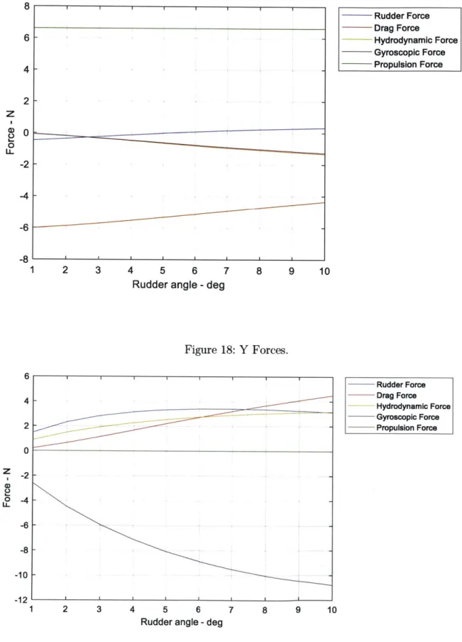
Here, RX, RY represent the rudder lift and drag forces, Dx, Dy represent the drag on the body, F, represents the propulsion force, Hx, Hy represent the body hydrodynamic forces, and Gx, Gy are the gyroscopic forces. Analytical expressions for these forces are shown in equations (91)-(95). Figures 17-19 show how the forces and moments in the X, Y, and N directions changed with respect to the rudder angle. The gyroscopic (also known as centrifugal) force in the Y direction is negative while all the other forces are positive and support this force. The moments diagram I Figure 19 shows the rudder and the drag moments, both of which are negative and supported by the positive hydrodynamic force.

A graphical representation of the free-body diagram for selected rudder angles (4' and 100) is shown in Figure 20 and Figure 21.

Figure 17: X Forces.

Rudder angle - deg

2 3 4 5 6 7 8 9 10

Rudder angle - deg

Figure 18: Y Forces. - .. II I I I I 7 8 9 10 Rudder Force Drag Force Hydrodynamic Force Gyroscopic Force Propulsion Force

z

z

Figure 19: N Moments.

Rudder angle - deg

Figure 20: 4' Rudder Angle Forces.

-7.12 Rudder Force -0 31Force 3.16 Gyroscopic Force Propulsion Force

8.&61

Figure 21: 100 Rudder Angle Forces.

-10.8 Rudder Force 0.3 i3

-4.35

5 Additional Fin for Maneuvering Improvement

To increase and improve the maneuvering performances, an extra vertical fin was introduced to the

model. An example of an optional fin configuration shown below.

Figure 22: REMUS with Additional Maneuvering Fin.

0.5 0.4 0.3 0.2 0.1 0 -0.1 -0.2 -0.3 -0.4 -0.5 -0.6 -0.4 -0.2 0 X -Axis 0.2 0.4 0.6

In the example above, the geometry of the added fin was set to be like the rudder fin. The fin chord

was tuned to set both the added fin and the rudder fin to be with the same plan area. After

re-computation of all the hydrodynamic coefficients due to the fin addition (excluding the Munk

moments that should stay as without fins at all), further simulations were conducted to investigate

the maneuvering performance in turning.

The following figures show the effect on the maneuverability of the vehicle following the addition of

a fin aligned in parallel to the vehicle centerline. Figure 23 compares the radii of turning for both

REMUS Fins

configurations, Figure 24 shows the yaw rate difference, Figure 25 shows the drift angle differences and Figure 26 shows the velocities of both configurations.

Figure 23: Comparison of Tactical Radii in Turning.

E 25 .2 20 'V cc W15

-10

Rudder angle - deg

Figure 24: Comparison of Yaw Rate in Turning.

o -.)15 -- 105 -I II I I I 1 2 3 4 5 6 7 8 9 10

Rudder angle - deg

Figure 25: Comparison of Drift Angle in Turning.

0)6-cc)

2

1 2 3 4 5 6 7 8 9 10

Rudder angle - deg

- - - Without added fin Fin Location=O Fin Location=0.1 Fin Location=0.2 Fin Location=0.3 Fin Location=0.4

- - Without added fin

Fin Location=O

Fin Location=0.1

Fin Location=0.2

Fin Location=0.3

Fin Location=0.4

- - - Without added fin Fin Location=0 Fin Location=0.1 Fin Location=0.2 Fin Location=0.3 Fin Location=0.4

Figure 26: Comparison of Final Surge Velocities.

. - - - Without added fin

Fin Location=0 - 1.35 - Fin Location=0.1 0 _ Fin Location=0.2 > 1.3 - _{Fin Location=0.3} (D

2'1.25 -

Rudder angle - deg

Careful analysis of the radius of turning and yaw rate results shows that for the configuration above, the addition of a fin, compared to a fin-less configuration at fin location x = 0, improved neither the turning radius nor the yaw rate. Nevertheless, moving the fin forwards from the center of gravity improves both properties. The drift angles with the fins are smaller than drift angles without fins and increases as the fin moved forward with respect to the center of gravity. Surge velocity exhibits same trend. Furthermore, as the fin moves forward (Figure 27 and Figure 28), the total hydrodynamic force increases and moves forward s well, the rudder lift force becomes larger, the fin lift force becomes smaller, and the Y drag force also becomes larger.