Measurement of the photon identification efficiencies with the ATLAS detector using LHC Run-1 data

(1)

arXiv:1606.01813v2 [hep-ex] 13 Dec 2016

EUROPEAN ORGANISATION FOR NUCLEAR RESEARCH (CERN)

Eur. Phys. J. C 76 (2016) 666

DOI:10.1140/epjc/s10052-016-4507-9

CERN-EP-2016-110 14th December 2016

Measurement of the photon identification

e

_{fficiencies with the ATLAS detector using LHC}

Run-1 data

The ATLAS Collaboration

The algorithms used by the ATLAS Collaboration to reconstruct and identify prompt photons are described. Measurements of the photon identification efficiencies are reported, using 4.9 fb−1of pp collision data collected at the LHC at √s = 7 TeV and 20.3 fb−1at √s = 8 TeV. The efficiencies are measured separately for converted and unconverted photons, in four dif-ferent pseudorapidity regions, for transverse momenta between 10 GeV and 1.5 TeV. The results from the combination of three data-driven techniques are compared to the predic-tions from a simulation of the detector response, after correcting the electromagnetic shower momenta in the simulation for the average differences observed with respect to data. Data-to-simulation efficiency ratios used as correction factors in physics measurements are determ-ined to account for the small residual efficiency differences. These factors are measured with uncertainties between 0.5% and 10% in 7 TeV data and between 0.5% and 5.6% in 8 TeV data, depending on the photon transverse momentum and pseudorapidity.

c

2016 CERN for the benefit of the ATLAS Collaboration.

(2)

1 Introduction

Several physics processes occurring in proton–proton collisions at the Large Hadron Collider (LHC) produce final states with prompt photons, i.e. photons not originating from hadron decays. The main contributions come from non-resonant production of photons in association with jets or of photon pairs, with cross sections respectively of the order of tens of nanobarns or picobarns [1–6]. The study of such final states, and the measurement of their production cross sections, are of great interest as they probe the perturbative regime of QCD and can provide useful information about the parton distribution functions of the proton [7]. Prompt photons are also produced in rarer processes that are key to the LHC physics programme, such as diphoton decays of the Higgs boson discovered with a mass near 125 GeV, produced with a cross section times branching ratio of about 20 fb at √s = 8 TeV [8]. Finally, some expected signatures of physics beyond the Standard Model (SM) are characterised by the presence of prompt photons in the final state. These include resonant photon pairs from graviton decays in models with extra spatial dimensions [9], pairs of photons accompanied by large missing transverse momentum produced

(3)

in the decays of pairs of supersymmetric particles [10] and events with highly energetic photons and jets from decays of excited quarks or other exotic scenarios [11].

The identification of prompt photons in hadronic collisions is particularly challenging since an over-whelming majority of reconstructed photons is due to background photons. These are usually real photons originating from hadron decays in processes with larger cross sections than prompt-photon production. An additional smaller component of background photon candidates is due to hadrons producing in the detector energy deposits that have characteristics similar to those of real photons.

Prompt photons are separated from background photons in the ATLAS experiment by means of selec-tions on quantities describing the shape and properties of the associated electromagnetic showers and by requiring them to be isolated from other particles in the event. An estimate of the efficiency of the photon identification criteria can be obtained from Monte Carlo (MC) simulation. Such an estimate, however, is subject to large,_{O(10%), systematic uncertainties. These uncertainties arise from limited knowledge} of the detector material, from an imperfect description of the shower development and from the detector response [1]. Ultimately, for high-precision measurements and for accurate comparisons with the predic-tions from the SM or from theories beyond the SM, a determination of the photon identification efficiency with an uncertainty ofO(1%) or smaller is needed in a large energy range from 10 GeV to several TeV. This can only be achieved through the use of data control samples. However, this can present several difficulties since there is no single physics process that produces a pure sample of prompt photons in a large transverse momentum (ET) range.

In this document, the reconstruction and identification of photons by the ATLAS detector are described, as well as the measurements of the identification efficiency. This study considers both photons that do (called converted photons in the following) or do not convert (called unconverted photons in the following) to electron-positron pairs in the detector material upstream of the ATLAS electromagnetic calorimeter. The measurements use the full Run-1 pp collision dataset recorded at centre-of-mass energies of 7 and 8 TeV. The details of the selections and the results are given for the data collected in 2012 at √s = 8 TeV. The same algorithms are applied with minor differences to the √s = 7 TeV data collected in 2011.

To overcome the difficulties arising from the absence of a single, pure control sample of prompt photons over a large ET range, three different data-driven techniques are used. A first method selects photons from radiative decays of the Z boson, i.e. Z _{→ ℓℓγ (Radiative Z method). A second one extrapolates} photon properties from electrons and positrons from Z boson decays by exploiting the similarity of the photon and electron interactions with the ATLAS electromagnetic calorimeter (Electron Extrapolation method). A third approach exploits a technique to determine the fraction of background present in a sample of isolated photon candidates (Matrix Method). Each of these techniques can measure the photon identification efficiency in complementary but overlapping ET regions with varying precision.

This document is organised as follows. After an overview of the ATLAS detector in Sect.2, the photon reconstruction and identification algorithms used in ATLAS are detailed in Sect.3. Section4 summar-ises the data and simulation samples used and describes the corrections applied to the simulated photon shower shapes in order to improve agreement with the data. In Sect.5the three data-driven approaches to the measurement of the photon identification efficiency are described, listing their respective sources of uncertainty and the precision reached in the relevant ET ranges. The results obtained with the √s = 8 TeV data collected in 2012, their consistency in the overlapping ET intervals and the comparison to the MC predictions are presented in Sect.6. Results obtained for the identification criteria used during the 2011 data-taking period at √s = 7 TeV are described in Sect.7. Finally, Sect.8discusses the impact of multiple inelastic interactions in the same beam crossing on the photon identification efficiency.

(4)

2 ATLAS detector

The ATLAS experiment [12] is a multi-purpose particle detector with approximately forward-backward symmetric cylindrical geometry and nearly 4π coverage in solid angle.1

The inner tracking detector (ID), surrounded by a thin superconducting solenoid providing a 2 T axial magnetic field, provides precise reconstruction of tracks within a pseudorapidity range_{|η| . 2.5. The} innermost part of the ID consists of a silicon pixel detector (50.5 mm < r < 150 mm) providing typic-ally three measurement points for charged particles originating in the beam-interaction region. The layer closest to the beam pipe (referred to as the b-layer in this paper) contributes significantly to precision vertexing and provides discrimination between prompt tracks and photon conversions. A semiconductor tracker (SCT) consisting of modules with two layers of silicon microstrip sensors surrounds the pixel detector, providing typically eight hits per track at intermediate radii (275 mm < r < 560 mm). The out-ermost region of the ID (563 mm < r < 1066 mm) is covered by a transition radiation tracker (TRT) con-sisting of straw drift tubes filled with a xenon gas mixture, interleaved with polypropylene/polyethylene transition radiators. For charged particles with transverse momentum pT > 0.5 GeV within its pseu-dorapidity coverage (_{|η| . 2), the TRT provides typically 35 hits per track. The distinction between} trans-ition radiation (low-energy photons emitted by electrons traversing the radiators) and tracking signals is obtained on a straw-by-straw basis using separate low and high thresholds in the front-end electronics. The inner detector allows an accurate reconstruction and transverse momentum measurement of tracks from the primary proton–proton collision region. It also identifies tracks from secondary vertices, per-mitting the efficient reconstruction of photon conversions up to a radial distance of about 80 cm from the beamline.

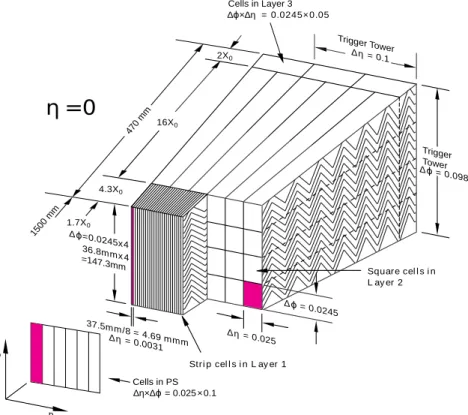
The solenoid is surrounded by a high-granularity lead/liquid-argon (LAr) sampling electromagnetic (EM) calorimeter with an accordion geometry. The EM calorimeter measures the energy and the position of electromagnetic showers with_{|η| < 3.2. It is divided into a barrel section, covering the pseudorapidity} region|η| < 1.475, and two end-cap sections, covering the pseudorapidity regions 1.375 < |η| < 3.2. The transition region between the barrel and the end-caps, 1.37 < |η| < 1.52, has a large amount of material upstream of the first active calorimeter layer. The EM calorimeter is composed, for_{|η| < 2.5, of three} sampling layers, longitudinal in shower depth. The first layer has a thickness of about 4.4 radiation lengths (X0). In the ranges|η| < 1.4 and 1.5 < |η| < 2.4, the first layer is segmented into high-granularity strips in the η direction, with a typical cell size of 0.003_{× 0.0982 in ∆η × ∆φ in the barrel. For 1.4 < |η| < 1.5 and} 2.4 <|η| < 2.5 the η-segmentation of the first layer is coarser, and the cell size is ∆η×∆φ = 0.025×0.0982. The fine η granularity of the strips is sufficient to provide, for transverse momenta up to_{O(100 GeV), an} event-by-event discrimination between single photon showers and two overlapping showers coming from the decays of neutral hadrons, mostly π0 and η mesons, in jets in the fiducial pseudorapidity region |η| < 1.37 or 1.52 < |η| < 2.37. The second layer has a thickness of about 17 X0and a granularity of 0.025_{× 0.0245 in ∆η × ∆φ. It collects most of the energy deposited in the calorimeter by photon and} electron showers. The third layer has a granularity of 0.05× 0.0245 in ∆η × ∆φ and a depth of about 2 X0. It is used to correct for leakage beyond the EM calorimeter of high-energy showers. In front of the accordion calorimeter, a thin presampler layer, covering the pseudorapidity interval_{|η| < 1.8, is used to}

1_{ATLAS uses a right-handed coordinate system with its origin at the nominal interaction point (IP) in the centre of the detector} and the z-axis along the beam pipe. The x-axis points from the IP to the centre of the LHC ring, and the y-axis points upward. Cylindrical coordinates (r, φ) are used in the transverse plane, φ being the azimuthal angle around the beam pipe. The pseudorapidity is defined in terms of the polar angle θ as η = − ln tan(θ/2). The photon transverse momentum is ET= E/ cosh(η), where E is its energy.

(5)

correct for energy loss upstream of the calorimeter. The presampler consists of an active LAr layer with a thickness of 1.1 cm (0.5 cm) in the barrel (end-cap) and has a granularity of ∆η× ∆φ = 0.025 × 0.0982. The material upstream of the presampler has a thickness of about 2 X0 for |η| < 0.6. In the region 0.6 < |η| < 0.8 this thickness increases linearly from 2 X0 to 3 X0. For 0.8 < |η| < 1.8 the material thickness is about or slightly larger than 3 X0, with the exception of the transition region between the barrel and the end-caps and the region near _{|η| = 1.7, where it reaches 5–6 X0}. A sketch of a barrel module of the electromagnetic calorimeter is shown in Fig.1.

The hadronic calorimeter surrounds the EM calorimeter. It consists of an iron–scintillator tile calorimeter in the central region (_{|η| < 1.7), and LAr sampling calorimeters with copper and tungsten absorbers in the} end-cap (1.5 <|η| < 3.2) and forward (3.1 < |η| < 4.9) regions.

The muon spectrometer surrounds the calorimeters. It consists of three large superconducting air-core toroid magnets, each with eight coils, a system of precision tracking chambers (_{|η| < 2.7), and fast} tracking chambers (|η| < 2.4) for triggering.

A three-level trigger system selects events to be recorded for offline analysis. A coarser readout granu-larity (corresponding to the “towers” of Fig.1) is used by the first-level trigger, while the full detector granularity is exploited by the higher-level trigger. To reduce the data acquisition rate of low-threshold triggers, used for collecting various control samples, prescale factors (N) can be applied to each trigger, such that only 1 in N events passing the trigger causes an event to be accepted at that trigger level.

∆ ϕ = 0.0₂₄₅ ∆ η = 0.025 37.5mm_{/8 = 4.69} mmm ∆ η = 0.0031 ∆ ϕ=0.02_45x4 36.8mmx Trigger To_wer ∆ ϕ = 0.0982 ∆ η = 0.1 16X0 4.3X0 2X0 1500 mm 470 m m η ϕ

η =0

Stri p cel l s i n L ay er 1 Square cel l s i n L ay er 2 1.7X0 Cells in Layer 3 ∆ϕ×∆η = 0.0245× 0.05 Cells in PS ∆η×∆ϕ = 0.025 × 0.1 Trigger Tower =147.3m_m4

Figure 1: Sketch of a barrel module (located at η = 0) of the ATLAS electromagnetic calorimeter. The different longitudinal layers (one presampler, PS, and three layers in the accordion calorimeter) are depicted. The granularity in η and φ of the cells of each layer and of the trigger towers is also shown.

(6)

3 Photon reconstruction and identification

3.1 Photon reconstruction

The electromagnetic shower, originating from an energetic photon’s interaction with the EM calorimeter, deposits a significant amount of energy in a small number of neighbouring calorimeter cells. As photons and electrons have very similar signatures in the EM calorimeter, their reconstruction proceeds in parallel. The electron reconstruction, including a dedicated, cluster-seeded track-finding algorithm to increase the efficiency for the reconstruction of low-momentum electron tracks, is described in Ref. [13]. The reconstruction of unconverted and converted photons proceeds in the following way:

• seed clusters of EM calorimeter cells are searched for;

• tracks reconstructed in the inner detector are loosely matched to seed clusters;

• tracks consistent with originating from a photon conversion are used to create conversion vertex candidates;

• conversion vertex candidates are matched to seed clusters;

• a final algorithm decides whether a seed cluster corresponds to an unconverted photon, a converted photon or a single electron based on the matching to conversion vertices or tracks and on the cluster and track(s) four-momenta.

In the following the various steps of the reconstruction algorithms are described in more detail.

The reconstruction of photon candidates in the region|η| < 2.5 begins with the creation of a preliminary set of seed clusters of EM calorimeter cells. Seed clusters of size ∆η_{× ∆φ = 0.075× 0.123 with transverse} momentum above 2.5 GeV are formed by a sliding-window algorithm [14]. After an energy comparison, duplicate clusters of lower energy are removed from nearby seed clusters. From MC simulations, the efficiency of the initial cluster reconstruction is estimated to be greater than 99% for photons with ET > 20 GeV.

Once seed clusters are reconstructed, a search is performed for inner detector tracks [15, 16] that are loosely matched to the clusters, in order to identify and reconstruct electrons and photon conversions. Tracks are loosely matched to a cluster if the angular distance between the cluster barycentre and the extrapolated track’s intersection point with the second sampling layer of the calorimeter is smaller than 0.05 (0.2) along φ in the direction of (opposite to) the bending of the tracks in the magnetic field of the ATLAS solenoid, and smaller than 0.05 along η for tracks with hits in the silicon detectors, i.e. the pixel and SCT detectors. Tracks with hits in the silicon detectors are extrapolated from the point of closest approach to the primary vertex, while tracks without hits in the silicon detectors are extrapolated from the last measured point. The track is extrapolated to the position corresponding to the expected maximum energy deposit for EM showers. To efficiently select low-momentum tracks that may have suffered significant bremsstrahlung losses before reaching the calorimeter, a similar matching procedure is applied after rescaling the track momentum to the measured cluster energy. The previous matching requirements are applied except that the φ difference in the direction of bending should be smaller than 0.1. Tracks that are loosely matched to a cluster and with hits in the silicon detectors are refitted with a Gaussian-sum-filter technique [17,18], to improve the track parameter resolution, and are retained for the reconstruction of electrons and converted photons.

(7)

“Double-track” conversion vertex candidates are reconstructed from pairs of oppositely charged tracks in the ID that are likely to be electrons. For each track the likelihood to be an electron, based on high-threshold hits and time-over-high-threshold of low-high-threshold hits in the TRT, is required to be at least 10% (80%) for tracks with (without) hits in the silicon detectors. Since the tracks of a photon conversion are parallel at the place of conversion, geometric requirements are used to select the track pairs. Track pairs are classified into three categories, whether both tracks (Si–Si), none (TRT–TRT) or only one of them (Si–TRT) have hits in the silicon detectors. Track pairs fulfilling the following requirements are retained:

• ∆ cot θ between the two tracks (taken at the tracks’ points of closest approach to the primary vertex) is less than 0.3 for Si–Si track pairs and 0.5 for track pairs with at least one track without hits in the silicon detectors. This requirement is not applied for TRT–TRT track pairs with both tracks within |η| < 0.6.

• The distance of closest approach between the two tracks is less than 10 mm for Si–Si track pairs and 50 mm for track pairs with at least one track without hits in the silicon detectors.

• The difference between the sum of the radii of the helices that can be constructed from the electron and positron tracks and the distance between the centres of the two helices is between−5 and 5 mm, between_{−50 and 10 mm, or between −25 and 10 mm, for Si–Si, TRT–TRT and Si–TRT track pairs,} respectively.

• ∆φ between the two tracks (taken at the estimated vertex position before the conversion vertex fit) is less than 0.05 for Si–Si track pairs and 0.2 for tracks pairs with at least one track without hits in the silicon detectors.

A constrained conversion vertex fit with three degrees of freedom is performed using the five measured helix parameters of each of the two participating tracks with the constraint that the tracks are parallel at the vertex. Only the vertices satisfying the following requirements are retained:

• The χ2of the conversion vertex fit is less than 50. This loose requirement suppresses fake candid-ates from random combination of tracks while being highly efficient for true photon conversions. • The radius of the conversion vertex, defined as the distance from the vertex to the beamline in the

transverse plane, is greater than 20 mm, 70 mm or 250 mm for vertices from Si–Si, Si–TRT and TRT–TRT track pairs, respectively.

• The difference in φ between the vertex position and the direction of the reconstructed conversion is less than 0.2.

The efficiency to reconstruct photon conversions as double-track vertex candidates decreases significantly for conversions taking place in the outermost layers of the ID. This effect is due to photon conversions in which one of the two produced electron tracks is not reconstructed either because it is very soft (asym-metric conversions where one of the two tracks has pT < 0.5 GeV), or because the two tracks are very close to each other and cannot be adequately separated. For this reason, tracks without hits in the b-layer that either have an electron likelihood greater than 95%, or have no hits in the TRT, are considered as “single-track” conversion vertex candidates. In this case, since a conversion vertex fit cannot be per-formed, the conversion vertex is defined to be the location of the first measurement of the track. Tracks which pass through a passive region of the b-layer are not considered as single-track conversions unless they are missing a hit in the second pixel layer.

(8)

As in the loose track matching, the matching of the conversion vertices to the clusters relies on an extra-polation of the conversion candidates to the second sampling layer of the calorimeter, and the comparison of the extrapolated η and φ coordinates to the η and φ coordinates of the cluster centre. The details of the extrapolation depend on the type of the conversion vertex candidate.

• For double-track conversion vertex candidates for which the track transverse momenta differ by less than a factor of four from each other, each track is extrapolated to the second sampling layer of the calorimeter and is required to be matched to the cluster.

• For double-track conversion vertex candidates for which the track transverse momenta differ by more than a factor of four from each other, the photon direction is reconstructed from the electron and positron directions determined by the conversion vertex fit, and used to perform a straight-line extrapolation to the second sampling layer of the calorimeter, as expected for a neutral particle. • For single-track conversion vertex candidates, the track is extrapolated from its last measurement. Conversion vertex candidates built from tracks with hits in the silicon detectors are considered matched to a cluster if the angular distance between the extrapolated conversion vertex candidate and the cluster centre is smaller than 0.05 in both η and φ. If the extrapolation is performed for single-track conversions, the window in φ is increased to 0.1 in the direction of the bending. For tracks without hits in the silicon detectors, the matching requirements are tighter:

• The distance in φ between the extrapolated track(s) and the cluster is less than 0.02 (0.03) in the direction of (opposite to) the bending. In the case where the conversion vertex candidate is extra-polated as a neutral particle, the distance is required to be less than 0.03 on both sides.

• The distance in η between the extrapolated track(s) and the cluster is less than 0.35 and 0.2 in the barrel and end-cap sections of the TRT, respectively. The criteria are significantly looser than in the φ direction since the TRT does not provide a measurement of the pseudorapidity in its barrel section. In the case that the conversion vertex candidate is extrapolated as a neutral particle, the distance is required to be less than 0.35.

In the case of multiple conversion vertex candidates matched to the same cluster, the final conversion vertex candidate is chosen as follows:

• preference is given to double-track candidates over single-track candidates;

• if both conversion vertex candidates are formed from the same number of tracks, preference is given to the candidate with more tracks with hits in the silicon detectors;

• if the conversion vertex candidates are formed from the same number of tracks with hits in the silicon detectors, preference is given to the vertex candidate with smaller radius.

The final arbitration between the unconverted photon, converted photon and electron hypotheses for the reconstructed EM clusters is performed in the following way [19]:

• Clusters to which neither a conversion vertex candidate nor any track has been matched during the electron reconstruction are considered unconverted photon candidates.

• Electromagnetic clusters matched to a conversion vertex candidate are considered converted photon candidates. For converted photon candidates that are also reconstructed as electrons, the electron track is evaluated against the track(s) originating from the conversion vertex candidate matched to the same cluster:

(9)

1. If the track coincides with a track coming from the conversion vertex, the converted photon candidate is retained.

2. The only exception to the previous rule is the case of a double-track conversion vertex can-didate where the coinciding track has a hit in the b-layer, while the other track lacks one (for this purpose, a missing hit in a disabled b-layer module is counted as a hit2).

3. If the track does not coincide with any of the tracks assigned to the conversion vertex candid-ate, the converted photon candidate is removed, unless the track pT is smaller than the pT of the converted photon candidate.

• Single-track converted photon candidates are recovered from objects that are only reconstructed as electron candidates with pT > 2 GeV and E/p < 10 (E being the cluster energy and p the track momentum), if the track has no hits in the silicon detectors.

• Unconverted photon candidates are recovered from reconstructed electron candidates if the electron candidate has a corresponding track without hits in the silicon detectors and with pT < 2 GeV, or if the electron candidate is not considered as single-track converted photon and its matched track has a transverse momentum lower than 2 GeV or E/p greater than 10. The corresponding electron candidate is then removed from the event. Using this procedure around 85% of the unconverted photons erroneously categorised as electrons are recovered.

From MC simulations, 96% of prompt photons with ET > 25 GeV are expected to be reconstructed as photon candidates, while the remaining 4% are incorrectly reconstructed as electrons but not as photons. The reconstruction efficiencies of photons with transverse momenta of a few tens of GeV (relevant for the search for Higgs boson decays to two photons) are checked in data with a technique described in Ref. [20]. The results point to inefficiencies and fake rates that exceed by up to a few percent the predictions from MC simulation. The efficiency to reconstruct photon conversions decreases at high ET (> 150 GeV), where it becomes more difficult to separate the two tracks from the conversions. Such conversions with very close-by tracks are often not recovered as single-track conversions because of the tighter selections, including the transition radiation requirement, applied to single-track conversion candidates. The overall photon reconstruction efficiency is thus reduced to about 90% for ETaround 1 TeV.

The final photon energy measurement is performed using information from the calorimeter, with a cluster size that depends on the photon classification.3 In the barrel, a cluster of size ∆η× ∆φ = 0.075 × 0.123 is used for unconverted photon candidates, while a cluster of size 0.075× 0.172 is used for converted photon candidates to compensate for the opening between the conversion products in the φ direction due to the magnetic field of the ATLAS solenoid. In the end-cap, a cluster size of 0.125× 0.123 is used for all candidates. The photon energy calibration, which accounts for upstream energy loss and both lateral and longitudinal leakage, is based on the same procedure that is used for electrons [20,21] but with different calibration factors for converted and unconverted photon candidates. In the following the photon transverse momentum ET is computed from the photon cluster’s calibrated energy E and the pseudorapidity η2 of the barycentre of the cluster in the second layer of the EM calorimeter as ET =

E/ cosh(η2).

2_{About 6.3% of the b-layer modules were disabled at the end of Run 1 due to individual module failures like low-voltage or} high-voltage powering faults or data transmission faults. During the shutdown following the end of Run 1, repairs reduced the b-layer fault fraction to 1.4%

3_{For converted photon candidates, the energy calibration procedure uses the following as additional inputs: (i) p}

T/ET and the momentum balance of the two conversion tracks if both tracks are reconstructed by the silicon detectors, and (ii) the conversion radius for photon candidates with transverse momentum above 3 GeV.

(10)

3.2 Photon identification

To distinguish prompt photons from background photons, photon identification with high signal efficiency and high background rejection is required for transverse momenta from 10 GeV to the TeV scale. Photon identification in ATLAS is based on a set of cuts on several discriminating variables. Such variables, listed in Table1and described in AppendixA, characterise the lateral and longitudinal shower development in the electromagnetic calorimeter and the shower leakage fraction in the hadronic calorimeter. Prompt photons typically produce narrower energy deposits in the electromagnetic calorimeter and have smaller leakage to the hadronic one compared to background photons from jets, due to the presence of additional hadrons near the photon candidate in the latter case. In addition, background candidates from isolated π0 _{→ γγ decays – unlike prompt photons – are often characterised by two separate local energy maxima} in the finely segmented strips of the first layer, due to the small separation between the two photons. The distributions of the discriminating variables for both the prompt and background photons are affected by additional soft pp interactions that may accompany the hard-scattering collision, referred to as in-time pile-up, as well as by out-of-time pile-up arising from bunches before or after the bunch where the event of interest was triggered. Pile-up results in the presence of low-ET activity in the detector, including energy deposition in the electromagnetic calorimeter. This effect tends to broaden the distributions of the discriminating variables and thus to reduce the separation between prompt and background photon candidates.

Two reference selections, a loose one and a tight one, are defined. The loose selection is based only on shower shapes in the second layer of the electromagnetic calorimeter and on the energy deposited in the hadronic calorimeter, and is used by the photon triggers. The loose requirements are designed to provide a high prompt-photon identification efficiency with respect to reconstruction. Their efficiency rises from 97% at Eγ_T = 20 GeV to above 99% for Eγ_T > 40 GeV for both the converted and unconverted photons, and the corresponding background rejection factor is about 1000 [19]. The rejection factor is defined as the ratio of the number of initial jets with pT > 40 GeV in the acceptance of the calorimeter to the number of reconstructed background photon candidates satisfying the identification criteria. The tight selection adds information from the finely segmented strip layer of the calorimeter, which provides good rejection of hadronic jets where a neutral meson carries most of the jet energy. The tight criteria are separately optimised for unconverted and converted photons to provide a photon identification efficiency of about 85% for photon candidates with transverse energy ET >40 GeV and a corresponding background rejection factor of about 5000 [19].

The selection criteria are different in seven intervals of the reconstructed photon pseudorapidity (0.0–0.6, 0.6–0.8, 0.8–1.15, 1.15–1.37, 1.52–1.81, 1.81–2.01, 2.01–2.37) to account for the calorimeter geometry and for different effects on the shower shapes from the material upstream of the calorimeter, which is highly non-uniform as a function of_|η|.

The photon identification criteria were first optimised prior to the start of the data-taking in 2010, on sim-ulated samples of prompt photons from γ+jet, diphoton and H → γγ events and samples of background photons in QCD multi-jet events [19]. Before the 2011 data-taking, the loose and the tight selections were loosened, without further re-optimisation, in order to reduce the systematic effects associated to the differences between the calorimetric variables measured from data and their description by the ATLAS simulation. Prior to the 8 TeV run in 2012, the identification criteria were reoptimised based on im-proved simulations in which the values of the shower shape variables are slightly shifted to improve the agreement with the data shower shapes, as described in the next section. To cope with the higher pile-up

(11)

Category Description Name loose tight

Acceptance _{|η| < 2.37, with 1.37 < |η| < 1.52 excluded} – X X

Hadronic leakage Ratio of ETin the first sampling layer of the hadronic calorimeter to ET of the EM cluster (used over the range_{|η| < 0.8 or |η| > 1.37)}

Rhad1 X X

Ratio of ET in the hadronic calorimeter to ET of the EM cluster (used over the range 0.8 <_{|η| < 1.37)}

Rhad X X

EM Middle layer Ratio of 3× 7 η × φ to 7 × 7 cell energies Rη X X

Lateral width of the shower w_η₂ X X

Ratio of 3×3 η × φ to 3×7 cell energies Rφ X

EM Strip layer Shower width calculated from three strips around the strip with maximum energy deposit

w_{s 3} X

Total lateral shower width ws tot X

Energy outside the core of the three central strips but within seven strips divided by energy within the three central strips

Fside X

Difference between the energy associated with the second maximum in the strip layer and the energy re-constructed in the strip with the minimum value found between the first and second maxima

∆E X

Ratio of the energy difference associated with the largest and second largest energy deposits to the sum of these energies

Eratio X

Table 1: Discriminating variables used for loose and tight photon identification.

expected during the 2012 data taking, the criteria on the shower shapes more sensitive to pile-up were relaxed while the others were tightened.

The discriminating variables that are most sensitive to pile-up are found to be the energy leakage in the hadronic calorimeter and the shower width in the second sampling layer of the EM calorimeter.

3.3 Photon isolation

The identification efficiencies presented in this article are measured for photon candidates passing an isol-ation requirement, similar to those applied to reduce hadronic background in cross-section measurements or searches for exotic processes with photons [1–6,8,9,11,22]. In the data taken at √s = 8 TeV, the calorimeter isolation transverse energy E_Tiso[23] is required to be lower than 4 GeV. This quantity is com-puted from positive-energy three-dimensional topological clusters of calorimeter cells [14] reconstructed in a cone of size ∆R = p(∆η)2_{+ (∆φ)}2_{= 0.4 around the photon candidate.}

(12)

The contributions to Eiso_T from the photon itself and from the underlying event and pile-up are subtrac-ted. The correction for the photon energy outside the cluster is computed as the product of the photon transverse energy and a coefficient determined from separate simulations of converted and unconverted photons. The underlying event and pile-up energy correction is computed on an event-by-event basis using the method described in Refs. [24] and [25]. A kTjet-finding algorithm [26,27] of size parameter

R = 0.5 is used to reconstruct all jets without any explicit transverse momentum threshold, starting from the three-dimensional topological clusters reconstructed in the calorimeter. Each jet is assigned an area Ajet via a Voronoi tessellation [28] of the η–φ space. According to this algorithm, every point within a jet’s assigned area is closer to the axis of that jet than to the axis of any other jet. The ambient transverse energy density ρUE(η) from pile-up and the underlying event is taken to be the median of the transverse energy densities pjet_T/Ajetof jets with pseudorapidity |η| < 1.5 or 1.5 < |η| < 3.0. The area of the photon isolation cone is then multiplied by ρUEto compute the correction to E_Tiso. The estimated ambient trans-verse energy fluctuates significantly event-by-event, reflecting the fluctuations in the underlying event and pile-up activity in the data. The typical size of the correction is 2 GeV in the central region and 1.5 GeV in the forward region.

A slight dependence of the identification efficiency on the isolation requirement is observed, as discussed in Section6.2.

4 Data and Monte Carlo samples

The data used in this study consist of the 7 TeV and 8 TeV proton–proton collisions recorded by the ATLAS detector during 2011 and 2012 in LHC Run 1. They correspond respectively to 4.9 fb−1 and 20.3 fb−1of integrated luminosity after requiring good data quality. The mean number of interactions per bunch crossing, µ, was 9 and 21 on average in the √s = 7 and 8 TeV datasets, respectively.

The Z boson radiative decay and the electron extrapolation methods use data collected with the lowest-threshold lepton triggers with prescale factors equal to one and thus exploit the full luminosity of Run 1. For the data collected in 2012 at √s = 8 TeV, the transverse momentum thresholds for single-lepton triggers are 25 (24) GeV for ℓ = e (µ), while those for dilepton triggers are 12 (13) GeV. For the data collected in 2011 at √s = 7 TeV, the transverse momentum thresholds for single-lepton triggers are 20 (18) GeV for ℓ = e (µ), while those for dilepton triggers are 12 (10) GeV. The matrix method uses events collected with single-photon triggers with loose identification requirements and large prescale factors, and thus exploits only a fraction of the total luminosity. Photons reconstructed near regions of the calorimeter affected by read-out or high-voltage failures [29] are rejected.

Monte Carlo samples are processed through a full simulation of the ATLAS detector response [30] using Geant4 [31] 4.9.4-patch04. Pile-up pp interactions in the same and nearby bunch crossings are included in the simulation. The MC samples are reweighted to reproduce the distribution of µ and the length of the luminous region observed in data (approximately 54 cm and 48 cm in the data taken at √s = 7 and 8 TeV, respectively). Samples of prompt photons are generated with PYTHIA8 [32,33]. Such samples include the leading-order γ + jet events from qg_{→ qγ and q¯q → gγ hard scattering, as well as prompt} photons from quark fragmentation in QCD dijet events. About 107 events are generated, covering the whole transverse momentum spectrum under study. Samples of background photons in jets are produced by generating with PYTHIA8 all tree-level 2_{→2 QCD processes, removing γ + jet events from quark} fragmentation. Between 1.2_{× 10}6_{and 5}_{× 10}6_Z_{→ ℓℓγ (ℓ = e, µ) events are generated with SHERPA [}₃₄_] or with POWHEG [35,36] interfaced to PHOTOS [37] for the modelling of QED final-state radiation and

(13)

to PYTHIA8 for showering, hadronisation and modelling of the underlying event. About 107Z(→ ℓℓ)+jet events are generated for both ℓ = e and ℓ = µ with each of the following three event generators: POWHEG interfaced to PYTHIA8; ALPGEN [38] interfaced to HERWIG [39] and JIMMY [40] for showering, hadronisation and modelling of the underlying event; and SHERPA. A sample of MC H→ Zγ events [41] is also used to compute the efficiency in the simulation for photons with transverse momentum between 10 and 15 GeV, since the Z _{→ ℓℓγ samples have a generator-level requirement on the minimum true} photon transverse momentum of 10 GeV which biases the reconstructed transverse momentum near the threshold. A two-dimensional reweighting of the pseudorapidity and transverse momentum spectra of the photons is applied to match the distributions of those reconstructed in Z _{→ ℓℓγ events. For the analysis} of √s = 7 TeV data, all simulated samples (photon+jet, QCD multi-jet, Z(_{→ ℓℓ)+jet and Z → ℓℓγ) are} generated with PYTHIA6.

For the analysis of 8 TeV data, the events are simulated and reconstructed using the model of the AT-LAS detector described in Ref. [20], based on an improved in situ determination of the passive material upstream of the electromagnetic calorimeter. This model is characterised by the presence of additional material (up to 0.6 radiation lengths) in the end-cap and a 50% smaller uncertainty in the material budget with respect to the previous model, which is used for the study of 7 TeV data.

The distributions of the photon transverse shower shapes in the ATLAS MC simulation do not perfectly match the ones observed in data. While the shapes of these distributions in the simulation are rather similar to those found in the data, small systematic differences in their average values are observed. On the other hand, the longitudinal electromagnetic shower profiles are well described by the simulation. The differences between the data and MC distributions are parameterised as simple shifts and applied to the MC simulated values to match the distributions in data. These shifts are calculated by minimising the χ2between the data and the shifted MC distributions of photon candidates satisfying the tight iden-tification criteria and the calorimeter isolation requirement described in the previous section. The shifts are computed in intervals of the reconstructed photon pseudorapidity and transverse momentum. The pseudorapidity intervals are the same as those used to define the photon selection criteria. The ET bin boundaries are 0, 15, 20, 25, 30, 40, 50, 60, 80, 100 and 1000 GeV. The typical size of the correction factors is 10% of the RMS of the distribution of the corresponding variable in data. For the variable Rη, for which the level of agreement between the data and the simulation is worst, the size of the correc-tion factors is 50% of the RMS of the distribucorrec-tion. The corresponding correccorrec-tion to the prompt-photon efficiency predicted by the simulation varies with pseudorapidity between −10% and −5% for photon transverse momenta close to 10 GeV, and approaches zero for transverse momenta above 50 GeV. Two examples of the simulated discriminating variable distributions before and after corrections, for con-verted photon candidates originating from Z boson radiative decays, are shown in Fig.2. For comparison, the distributions observed in data for candidates passing the Z boson radiative decay selection illustrated in Sect.5.1, are also shown. Better agreement between the shower shape distributions in data and in the simulation after applying such corrections is clearly visible.

5 Techniques to measure the photon identification e

_fficiency

The photon identification efficiency, εID, is defined as the ratio of the number of isolated photons passing the tight identification selection to the total number of isolated photons. Three data-driven techniques are developed in order to measure this efficiency for reconstructed photons over a wide transverse momentum range.

(14)

side F 0 0.1 0.2 0.3 0.4 0.5 0.6 0.7 0.8 0.9 1 Entries/0.02 1 10 2 10 3 10 4 10 data γ ll → Z corrected MC γ ll → Z uncorrected MC γ ll → Z -1 Ldt=20.3 fb ∫ =8 TeV, s γ Converted ATLAS (a) s3 w 0 0.1 0.2 0.3 0.4 0.5 0.6 0.7 0.8 0.9 1 Entries/0.02 1 10 2 10 3 10 data γ ll → Z corrected MC γ ll → Z uncorrected MC γ ll → Z -1 Ldt=20.3 fb ∫ =8 TeV, s γ Converted ATLAS (b)

Figure 2: Distributions of the calorimetric discriminating variables (a) Fsideand (b) ws 3for converted photon

can-didates with ET>20 GeV and|η| < 2.37 (excluding 1.37 < |η| < 1.52) selected from Z → ℓℓγ events obtained from

the 2012 data sample (dots). The distributions for true photons from simulated Z _{→ ℓℓγ events (blue hatched and} red hollow histograms) are also shown, after reweighting their two-dimensional ETvs η distributions to match that

of the data candidates. The blue hatched histogram corresponds to the uncorrected simulation and the red hollow one to the simulation corrected by the average shift between data and simulation distributions determined from the inclusive sample of isolated photon candidates passing the tight selection per bin of (η, ET) and for converted and

unconverted photons separately. The photon candidates must be isolated but no shower-shape criteria are applied. The photon purity of the data sample, i.e. the fraction of prompt photons, is estimated to be approximately 99%.

The Radiative Z method uses a clean sample of prompt, isolated photons from radiative leptonic decays of the Z boson, Z_{→ ℓℓγ, in which a photon produced from the final-state radiation of one of the two leptons} is selected without imposing any criteria on the photon discriminating variables. Given the luminosity of the data collected in Run 1, this method allows the measurement of the photon identification efficiency only for 10 GeV. ET . 80 GeV.

In the Electron Extrapolation method, a large and pure sample of electrons selected from Z→ ee decays with a tag-and-probe technique is used to deduce the distributions of the discriminating variables for photons by exploiting the similarity between the electron and the photon EM showers. Given the typical ET distribution of electrons from Z boson decays and the Run-1 luminosity, this method provides precise results for 30 GeV. ET . 100 GeV.

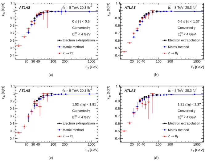
The Matrix Method uses the discrimination between prompt photons and background photons provided by their isolation from tracks in the ID to extract the sample purity before and after applying the tight iden-tification requirements. This method provides results for transverse momenta from 20 GeV to 1.5 TeV. The three measurements are performed for photons with pseudorapidity in the fiducial region of the EM calorimeter in which the first layer is finely segmented along η: _{|η| < 1.37 or 1.52 < |η| < 2.37.} The identification efficiency is measured as a function of ETin four pseudorapidity intervals: |η| < 0.6, 0.6 < |η| < 1.37, 1.52 < |η| < 1.81 and 1.81 < |η| < 2.37. Since there are not many data events with high-ET photons, the highest ET bin in which the measurement with the matrix method is performed corresponds to the large interval 250 GeV< ET < 1500 GeV (the upper limit corresponding to the transverse energy of the highest-ET selected photon candidate). In this range a majority of the photon candidates have transverse momenta below about 400 GeV (the ET distribution of the selected photon

(15)

candidates in this interval has an average value of 300 GeV and an RMS value of 70 GeV). However, from the simulation the photon identification efficiency is expected to be constant at the few per-mil level in this ETrange.

5.1 Photons from Z boson radiative decays

Radiative Z → ℓℓγ decays are selected by placing kinematic requirements on the dilepton pair, the invariant mass of the three particles in the final state and quality requirements on the two leptons. The reconstructed photon candidates are required to be isolated in the calorimeter but no selection is applied to their discriminating variables.

Events are collected using the lowest-threshold unprescaled single-lepton or dilepton triggers.

Muon candidates are formed from tracks reconstructed both in the ID and in the muon spectrometer [42], with transverse momentum larger than 15 GeV and pseudorapidity_{|η| < 2.4. The muon tracks are required} to have at least one hit in the innermost pixel layer, one hit in the other two pixel layers, five hits in the SCT, and at most two missing hits in the two silicon detectors. The muon track isolation, defined as the sum of the transverse momenta of the tracks inside a cone of size ∆R = p(∆η)2_{+ (∆φ)}2_{= 0.2 around the} muon, excluding the muon track, is required to be smaller than 10% of the muon pT.

Electron candidates are required to have ET > 15 GeV, and |η| < 1.37 or 1.52 < |η| < 2.47. Electrons are required to satisfy medium identification criteria [43] based on tracking and transition radiation in-formation from the ID, shower shape variables computed from the lateral and longitudinal profiles of the energy deposited in the EM calorimeter, and track–cluster matching quantities.

For both the electron and muon candidates, the longitudinal (z0) and transverse (d0) impact parameters of the reconstructed tracks with respect to the primary vertex with at least three associated tracks and with the largest P p2

T of the associated tracks are required to satisfy |z0| < 10 mm and |d0|/σd0 < 10,

respectively, where σd0 is the estimated d0uncertainty.

The Z→ ℓℓγ candidates are selected by requiring two opposite-sign charged leptons of the same flavour satisfying the previous criteria and one isolated photon candidate with ET > 10 GeV and |η| < 1.37 or 1.52 <_{|η| < 2.37. An angular separation ∆R > 0.2 (0.4) between the photon and each of the two muons} (electrons) is required so that the energy deposited by the leptons in the calorimeter does not bias the photon discriminating variables. In the selected events, the triggering leptons are required to match one (or in the case of dilepton triggered events, both) of the Z candidate’s leptons.

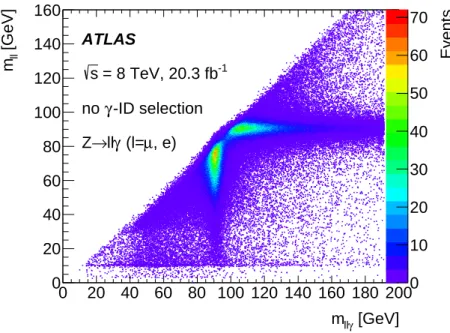
The two-dimensional distribution of the dilepton invariant mass, mℓℓ, versus the invariant mass of the three final-state particles, mℓℓγ, in events selected in √s = 8 TeV data is shown in Fig.3. The selected sample is dominated by Z +jet background events in which one jet is misreconstructed as a photon. These events, which have a cross section about three orders of magnitudes higher than ℓℓγ events, have mℓℓ ≈ mZ and mℓℓγ & mZ, while final-state radiation Z → ℓℓγ events have mℓℓ . mZ and mℓℓγ ≈ mZ, where mZ is the Z boson pole mass. To significantly reduce the Z +jet background, the requirements of 40 GeV < mℓℓ<83 GeV and 80 GeV < mℓℓγ<96 GeV are thus applied.

After the selection, about 54000 unconverted and about 19000 converted isolated photon candidates are selected in the Z_{→ µµγ channel, and 32000 unconverted and 12000 converted isolated photon candidates} are selected in the Z → eeγ channel. The residual background contamination from Z+jet events is estimated through a maximum-likelihood fit (called “template fit” in the following) to the mℓℓγdistribution

(16)

[GeV] γ ll m 0 20 40 60 80 100 120 140 160 180 200 [GeV]_ll m 0 20 40 60 80 100 120 140 160 Events 0 10 20 30 40 50 60 70 -1 = 8 TeV, 20.3 fb s -ID selection γ no , e) µ (l= γ ll → Z ATLAS

Figure 3: Two-dimensional distribution of mℓℓγ and mℓℓfor all reconstructed Z → ℓℓγ candidates after loosening

the selection applied to mℓℓγ and mℓℓ. No photon identification requirements are applied. Events from initial-state

(mℓℓ≈ mZ) and final-state (mℓℓγ ≈ mZ) radiation are clearly visible.

of selected events after discarding the 80 GeV < mℓℓγ<96 GeV requirement. The data are fit to a sum of the photon and background contributions. The photon and background mℓℓγ distributions (“templates”) are extracted from the Z → ℓℓγ and Z +jet simulations, corrected to take into account known data–MC differences in the photon and lepton energy scales and resolution and in the lepton efficiencies. The signal and background yields are determined from the data by maximising the likelihood. Due to the small number of selected events in data and simulation, these fits are performed only for two photon transverse momentum intervals, 10 GeV < ET < 15 GeV and ET > 15 GeV, and integrated over the photon pseudorapidity, since the signal purity is found to be similar in the four photon_{|η| intervals within} statistical uncertainties.

Figure4shows the result of the fit for unconverted photon candidates with transverse momenta between 10 GeV and 15 GeV. The fraction of residual background in the region 80 GeV < mℓℓγ < 96 GeV decreases rapidly with the reconstructed photon transverse momentum, from≈ 10% for 10 GeV < ET < 15 GeV to≤ 2% for higher-ET regions. A similar fit is also performed for the subsample in which the photon candidates are required to satisfy the tight identification criteria.

The identification efficiency as a function of ET is estimated as the fraction of all the selected probes in a certain ET interval passing the tight identification requirements. For 10 GeV < ET < 15 GeV, both the numerator and denominator are corrected for the average background fraction determined from the template fit. For ET > 15 GeV, the background is neglected in the nominal result, and a systematic uncertainty is assigned as the difference between the nominal result and the efficiency that would be obtained taking into account the background fraction determined from the template fit in this ET region. Additional systematic uncertainties related to the signal and background mℓℓγdistributions are estimated by repeating the previous fits with templates extracted from alternative MC event generators (POWHEG interfaced to PHOTOS and PYTHIA8 for Z _{→ ℓℓγ and ALPGEN for Z+jet, Z → ℓℓ). The total relative} uncertainty in the efficiency, dominated by the statistical component, increases from 1.5–3% (depending

(17)

[GeV] γ µ µ m 60 65 70 75 80 85 90 95 100 105 110 ] -1 [GeV γµ µ dN/dm 10 2 10 3 10 4 10 data fit signal background signal region ATLAS -1 = 8 TeV, 20.3 fb s Unconvertedγ < 15 GeV T γ 10 < E 0.2)% ± Purity = (93.4

Figure 4: Invariant mass (mµµγ) distribution of events in which the unconverted photon has 10 GeV < ET<15 GeV,

selected in data at √s = 8 TeV after applying all the Z _{→ µµγ selection criteria except that on m}µµγ(black dots).

No photon identification requirements are applied. The solid black line represents the result of fitting the data distribution to a sum of the signal (red dashed line) and background (blue dotted line) invariant mass distributions obtained from simulations.

on η and whether the photon was reconstructed as a converted or an unconverted candidate) for 10 GeV < ET <15 GeV to 5–20% for ET >40 GeV.

5.2 Electron extrapolation

The similarity between the electromagnetic showers induced by isolated electrons and photons in the EM calorimeter is exploited to extrapolate the expected photon distributions of the discriminating variables. The photon identification efficiency is thus estimated from the distributions of the same variables in a pure and large sample of electrons with ET between 30 GeV and 100 GeV obtained from Z → ee decays using a tag-and-probe method [43]. Events collected with single-electron triggers are selected if they contain two opposite-sign electrons with ET > 25 GeV, |η| < 1.37 or 1.52 < |η| < 2.47, at least one hit in the pixel detector and seven hits in the silicon detectors, Eiso_T < 4 GeV and invariant mass 80 GeV < mee < 120 GeV. The tag electron is required to match the trigger object and to pass the tight electron identification requirements. A sample of about 9_{× 10}6 electron probes is collected. Its purity is determined from the meespectrum of the selected events by estimating the background, whose normalisation is extracted using events with mee > 120 GeV and whose shape is obtained from events in which the probe electron candidate fails both the isolation and identification requirements. The purity varies slightly with ETand|η|, but is always above 99%.

The differences between the photon and electron distributions of the discriminating variables are studied using simulated samples of prompt photons and electrons from Z _{→ ee decays, separately for converted} and unconverted photons. The shifts of the photon discriminating variables described in Sect.4are not

(18)

applied, since it is observed that the photon and electron distributions are biased in a similar way in the simulation.

Photon conversions produce electron–positron pairs which are usually sufficiently collimated to produce overlapping showers in the calorimeter, giving rise to single clusters with distributions of the discrim-inating variables similar to those of an isolated electron. The largest differences between electrons and converted photons are found in the Rφdistribution, due to the bending of electrons and positrons in oppos-ite directions in the r–φ plane, which leads to a broader Rφdistribution for converted photons. However, the Rφrequirement used for the identification of converted photons is relatively loose, and a test on MC simulated samples shows that, by directly applying the converted photon identification criteria to an elec-tron sample, the εIDobtained from electrons overestimates the efficiency for converted photons by at most 3%.

The showers induced by unconverted photons are more likely to begin later than those induced by elec-trons, and thus to be narrower in the first layer of the EM calorimeter. Additionally, the lack of photon-trajectory bending in the φ plane makes the Rφdistribution particularly different from that of electrons. Therefore, if the unconverted-photon selection criteria are directly applied to an electron sample, the εID obtained from these electrons is about 20–30% smaller than the efficiency for unconverted photons with the same pseudorapidity and transverse momentum.

To reduce such effects a mapping technique based on a Smirnov transformation [44] is used for both the unconverted and converted photons. For each discriminating variable x, the cumulative distribution functions (CDF) of simulated electrons and photons, CDFe(x) and CDFγ(x), are calculated. The trans-form f (x) is thus defined by CDFe(x) = CDFγ( f (x)). The discriminating variable of the electron probes selected in data can then be corrected on an event-by-event basis by applying the transform f (x) to obtain the expected one for photons in data. Figure5illustrates the process for one shower shape (Rφ). These Smirnov transformations are invariant under systematic shifts which are fully correlated between the elec-tron and photon distributions. Due to the differences in the|η| and ETdistributions of the source and target samples, the dependence of the shower shapes on_{|η|, ET}, and whether the photon was reconstructed as a converted or an unconverted candidate, this process is applied separately for converted and unconverted photons, and in various regions of ET and |η|. The efficiency of the identification criteria is determined from the extrapolated photon distributions of the discriminating variables.

The following three sources of systematic uncertainty are considered for this analysis:

• As the Smirnov transformations are obtained independently for each shower shape, the estimated photon identification efficiency can be biased if the correlations among the discriminating variables are significantly different between electrons and photons. Non-closure tests are performed on the simulation, comparing the identification efficiency of true prompt photons with the efficiency ex-trapolated from electron probes selected with the same requirement as in data and applying the extrapolation procedure. The differences between the true and extrapolated efficiencies are at the level of 1% or less, with a few exceptions for unconverted photons, for which maximum differences of 2% are found.

• The results are also affected by the uncertainties in the modelling of the shower shape distributions and correlations in the photon and electron simulations used to extract the mappings. The largest uncertainties in the distributions of the discriminating variables originate from limited knowledge of the material upstream of the calorimeter. The extraction of the mappings is repeated using alternative MC samples based on a detector simulation with a conservative estimate of additional material in front of the calorimeter [21]. This detector simulation is considered as conservative

(19)

φ R 0.4 0.5 0.6 0.7 0.8 0.9 1 1.1 pdf 6 − 10 5 − 10 4 − 10 3 − 10 2 − 10 1 −

10 45 GeV < ET < 50 GeV and 0 < |η| ≤ 0.6

electrons photons ATLAS Simulation (a) φ R 0.4 0.5 0.6 0.7 0.8 0.9 1 1.1 CDF 0 0.2 0.4 0.6 0.8 1 0.6 ≤ | η < 50 GeV and 0 < | T 45 GeV < E electrons photons ATLAS Simulation (b) (electrons) φ R 0.4 0.5 0.6 0.7 0.8 0.9 1 1.1 (photons)_φ R 0.7 0.75 0.8 0.85 0.9 0.95 1 1.05 1.1 0.6 ≤ | η < 50 GeV and 0 < | T 45 GeV < E Smirnov transform ATLAS Simulation (c) φ R 0.4 0.5 0.6 0.7 0.8 0.9 1 1.1 pdf 6 − 10 5 − 10 4 − 10 3 − 10 2 − 10 1 −

10 45 GeV < E_T < 50 GeV and 0 < |η| ≤ 0.6 transformed electrons

photons ATLAS Simulation

(d)

Figure 5: Diagram illustrating the process of Smirnov transformation. Rφis chosen as an example discriminating

variable whose distribution is particularly different between electrons and (unconverted) photons. The Rφ

probab-ility density function (pdf) in each sample (a) is used to calculate the respective CDF (b). From the two CDFs, a Smirnov transformation can be derived (c). Applying the transformation leads to an Rφdistribution of the

(20)

enough to cover any mismodelling of the distributions of the discriminating variables. The extracted εID differs from the nominal one by typically less than 1% for converted photons and 2% for unconverted ones, with maximum deviations of 2% and 3.5% in the worst cases, respectively. • Finally, the effect of a possible background contamination in the selected electron probes in data

is found to be smaller than 0.5% in all ET, |η| intervals for both the converted and unconverted photons.

The total uncertainty is dominated by its systematic component and ranges from 1.5% in the central region to 7.5% in the highest ETbin in the endcap region, with typical values of 2.5%.

5.3 Matrix method

An inclusive sample of about 7× 106_{isolated photon candidates is selected using single-photon triggers} by requiring at least one photon candidate with transverse momentum 20 GeV < ET < 1500 GeV and isolation energy Eiso_T < 4 GeV, matched to the photon trigger object passing the loose identification requirements.

The distribution of the track isolation of selected candidates in data is used to discriminate between prompt and background photon candidates, before and after applying the tight identification criteria. The track isolation variable used for the measurement of the efficiency of unconverted photon candidates, piso_T , is defined as the scalar sum of the transverse momenta of the tracks, with transverse momentum above 0.5 GeV and distance of closest approach to the primary vertex along z less than 0.5 mm, within a hollow cone of 0.1 < ∆R < 0.3 around the photon direction. For the measurement of the efficiency of the converted photon candidates, the track isolation variable νiso_trk is defined as the number of tracks, passing the previous requirements, within a hollow cone of 0.1 < ∆R < 0.4 around the photon direction. Unconverted photon candidates with piso_T < 1.2 GeV and converted photon candidates with νiso_trk = 0 are considered to be isolated from tracks. The track isolation variables and requirements were chosen to minimise the total uncertainty in the identification efficiency after including both the statistical and systematic components.

The yields of prompt and background photons in the selected sample (“ALL” sample), N_allS and NB_all, and in the sample of candidates satisfying the tight identification criteria (“PASS” sample), NS

pass and NpassB , are obtained by solving a system of four equations:

N_allT = N_allS + N_allB,

N_passT = N_passS + N_passB ,

N_allT,iso = εS_all_{× N}_allS + εB_all× NallB,

N_passT,iso = εS_pass_{× N}_passS + εB_pass× NpassB . (1) Here N_allT and N_passT are the total numbers of candidates in the ALL and PASS samples respectively, while N_allT,isoand NpassT,isoare the numbers of candidates in the ALL and PASS samples that pass the track isolation requirement. The quantities εS(B)_all and εS(B)_pass are the efficiencies of the track isolation requirements for prompt (background) photons in the ALL and PASS samples.

(21)

Equation (1) implies that the fractions fpassand fallof prompt photons in the ALL and in the PASS samples can be written as:

fpass = εpass− εBpass εS_pass_{− ε}B_pass fall = εall− εB_all εS_all_{− ε}B_all (2)

where εpass(all) = N_pass(all)T,iso /N_pass(all)T is the fraction of tight (all) photon candidates in data that satisfy the track isolation criteria.

The identification efficiency εID= NpassS /NallS is thus:

ε_ID= N T pass N_allT        ε_pass_{− ε}B_pass εS_pass_{− ε}B_pass               εall− εB_all εS_all_{− ε}B_all        −1 . (3)

The prompt-photon track isolation efficiencies, εS_alland εS_pass, are estimated from simulated prompt-photon events. The difference between the track isolation efficiency for electrons collected in data and simulation with a tag-and-probe Z → ee selection is taken as a systematic uncertainty. An additional systematic uncertainty in the prompt-photon track isolation efficiencies is estimated by conservatively varying the fraction of fragmentation photons in the simulation by_{±100%. The overall uncertainties in ε}S_alland εS_pass are below 1%.

The background-photon track isolation efficiencies, εB_all and εB_pass, are estimated from data samples en-riched in background photons. For the measurement of εB_all, the control sample of all photon candidates not meeting at least one of the tight identification criteria is used. In order to obtain εB_pass, a relaxed ver-sion of the tight identification criteria is defined. The relaxed tight selection consists of those candidates which fail at least one of the requirements on four discriminating variables computed from the energy in the cells of the first EM calorimeter layer (Fside, ws3, ∆E, Eratio), but satisfy the remaining tight identifica-tion criteria. The four variables which are removed from the tight selecidentifica-tion to define the relaxed tight one are computed from the energy deposited in a few strips of the first compartment of the LAr EM calori-meter near the one with the largest deposit and are chosen since they have negligible correlations with the photon isolation. Due to the very small correlation (few %) between the track isolation and these discrim-inating variables, the background-photon track isolation efficiency is similar for photons satisfying tight or relaxed tight criteria. The differences between the track isolation efficiencies for background photons satisfying tight or relaxed tight criteria are included in the systematic uncertainties. The contamination from prompt photons in the background enriched samples is accounted for in this procedure by using as an additional input the fraction of signal events passing or failing the relaxed tight requirements, as determined from the prompt-photon simulation. The fraction of prompt photons in the background con-trol samples decreases from about 20% to 1%, with increasing photon transverse momentum. The whole procedure is tested with a simulated sample of γ+jet and dijet events, and the difference between the true track isolation efficiency for background photons and the one estimated with this procedure is taken as a systematic uncertainty. An additional systematic uncertainty, due to the use of the prompt-photon simulation to estimate the fraction of signal photons in the background control regions, is estimated by re-calculating these fractions using alternative MC samples based on a detector simulation with a conser-vative estimate of additional material in front of the calorimeter. The typical total relative uncertainty in the background-photon track isolation efficiency is 2–4%.