Beta-ensembles with covariance

Beta-Ensembles with Covariance

by

Alexander Dubbs

A.B. Harvard University (2009)

Submitted to the Department of Mathematics

in partial fulfillment of the requirements for the degree of

Doctor of Philosophy in Applied Mathematics

at the

MASSACHUSETTS INSTITUTE OF TECHNOLOGY

June 2014

@2014

Alexander Dubbs. All rights reserved.

4 MSACHUSET & OF TECHNOLOGY

JUN 17 2014

LI BRARI ES

Author . 1' V

Certified by.

Signature redacted

- - -- to"

Department of Mathematics

April 18, 2014

Signature redacted

Alan Edelman

Professor

Thesis Supervisor

Signature redacted

A ccepted by ...

Peter Shor

Chairman, Applied Mathematics Committee

Beta-Ensembles with Covariance

by

Alexander Dubbs

Submitted to the Department of Mathematics on April 18, 2014, in partial fulfillment of the

requirements for the degree of

Doctor of Philosophy in Applied Mathematics

Abstract

This thesis presents analytic samplers for the ,3-Wishart and O-MANOVA ensembles with diagonal covariance. These generalize the /3-ensembles of Dumitriu-Edelman, Lippert, Killip-Nenciu, Forrester-Rains, and Edelman-Sutton, as well as the classical

3 = 1, 2,4 ensembles of James, Li-Xue, and Constantine. Forrester discovered a

sampler for the -Wishart ensemble around the same time, although our proof has key differences. We also derive the largest eigenvalue pdf for the /3-MANOVA case. In infinite-dimensional random matrix theory, we find the moments of the Wachter law, and the Jacobi parameters and free cumulants of the McKay and Wachter laws. We also present an algorithm that uses complex analysis to solve "The Moment Problem." It takes the first batch of moments of an analytic, compactly-supported distribution as input, and it outputs a fine discretization of that distribution.

Thesis Supervisor: Alan Edelman Title: Professor

Acknowledgments

I am grateful for the help of my adviser Alan Edelman. This thesis would not have

been possible without his patience and inspiration. Thanks to him I am a much better researcher than I was when I arrived at MIT. It was a priviledge to contribute to the fields of ,3-ensembles and infinite random matrix theory.

I am also grateful for the help of my coauthors Plamen Koev and Praveen

Venkatara-mana. Plamen's mhg software and Praveen's combinatorial skills helped push this thesis across the finish line.

I would also like to thank Marcelo Magnasco and Christopher Jones. Marcelo let

me into his lab while I was still a high school student and taught me to do compu-tational neuroscience research, culminating in a paper. Chris both kept me occupied with "bonus" problems and allowed me the opportunity to learn independently.

To my friends, it has been a wonderful experience living with you in Cambridge for the last nine years, you will all be missed.

Chapter 1

Introduction

1.1

Work on beta-ensembles to date.

We define a -ensemble to be a probability distribution with a continuous dimension parameter

/3

> 0 that adjusts the degree of Vandermonde repulsion among its

vari-ables. /3-ensembles are typically the eigenvalue, singular value, or generalized singular value distributions of finite random matrices with Gaussian entries. The three main ones are the Hermite, Laguerre, and Jacobi ensembles, see [12].

Hermite c. f7 JAi - A 1exp -

)

i<j

Laguerre c'

aFJIAi

- AjL exp f A -2ZAi

i<j i i=1

Jacobi cI3

a1a2

f

IA - A1j-3expJJ (Aalp(1 - Ai)a2-P) i<j

The

/

- 1, 2, 4 cases of these distributions are the eigenvalue distributions of

ensem-bles of real

(/

= 1), complex

(/

= 2), and quaternionic

(/

= 4) random matrices of Gaussians. Let X and Y denote a Gaussian random matrices over the reals, com-plexes, or quaternions, depending on /. In terms of the eigenvalue distribution, we have the correspondence:

There also exist finite Gaussian random matrix ensembles over the reals, complexes, or quaternions governed by a diagonal matrix of nonrandom tuning parameters, called the ensemble's "covariance." The two known ones are below, where gsvdc indicates the "cosine generalized singular values."

gsvdc (Y, XQ) = eig (Yty/(yty + QXtXQ> - ) 1/2

D and Q are diagonal matrices of tuning parameters, E = diag(- 1, ... , -) are singular

values, and C = diag(ci,..., cn) are cosine generalized singular values. see [10] and [11]. D n (m-n+1),3-1 2 - 2 Wishart svd (D1/2x) CW Fi 0 '3 (ZD i x Fo (3)(IY 2, D-1) c Q fl 1" C(-1 1 n" (1 - C2)-(p+n-2),3/2-1 MANOVA gsvdc (Y, XQ) M

H

R

x

fJi<j

|c - c|11Fo(3) (rn- .; c2(C2 - i)-1, Q2)

The hypergeometric functions pF (3) are defined in Chapter 2, Section 2.5 (and that

definition uses the Jack functions, which are in Section 2.4).

It is a natural question to ask, "For continuous 0 > 0, is there a matrix ensemble

that has a given 3-ensemble as its eigenvalue distribution?" In [12], Dumitriu and Edelman were the first to answer yes, in the cases of the Hermite and Laguerre ensemble. If we define the matrix B as it is below, eig(BBt) follows the Laguerre

ensemble, and it works for any 3 > 0. Xk's denote independent X-distributed variables

Hermite eig ((X + Xt)/2)

Laguerre eig (XXt)

with the correct degrees of freedom.

X2a

B X3(m-i) X2a-0

X,3 X2a-O(m-1)

This thesis' contributions to finite random matrix theory are analytic samplers for the /3-Wishart and /3-MANOVA ensembles with covariance for general

3

> 0. They

are not as simple as finding the eigenvalues of a matrix, instead, the eigenvalues of many matrices are needed to produce the samples, which are proven to come from the exactly correct distributions. In addition, we contribute the probability distribution function of the largest eigenvalue of the 3-MANOVA ensemble, which we check with the software mhg [43]. Chapter 2 (originally in [10]) is concerned with the 3-Wishart ensemble, which was discovered around the same time by Forrester [27], and Chapter

3 (originally in [11]) is concerned with the /-MANOVA ensemble. Most work to date

on matrix models for 3-ensembles is described below:

Laguerre/Wishart Models

Q = I (Laguerre) D general (Wishart)

Fisher [24] (1939), I3 1 Hsu [33] (1939), James [36] (1960) Roy [61] (1939) 3 2 James [37] (1964) James [37] (1964) 3 4 Li-Xue [45] (2009) Li-Xue [45] (2009) Forrester [27] (2011), 3 > 0 [12ti(Ed02) , Dubbs-Edelman-Koev-Venkatarmana, [12] (2002)[10] (2013)

Jacobi/MANOVA Models

Q = I (Jacobi) Q general (MANOVA)

Fisher [24] (1939), Girshick [29] (1939), Constantine

3=

1 Hsu [33] (1939), Mood [51] (1951), (unpublished,

Olkin-Roy [55] (1954), Roy [61] (1939) found in [37] (1964))

/

= 2 James [37] (1964)

-Lippert [46] (2003),

/

> 0 Killip-Nenciu [40] (2004), Dubbs-Edelman [11] (2014)

Forrester-Rains [28] (2005), Edelman-Sutton [21] (2008)

The Hermite ensemble does not, as of this writing, have a generalization using a covariance matrix. In addition, a matrix model for the /-circular ensemble was were proven to work by [40]. The samplers for the /3-Wishart and /3-MANOVA ensembles are described below. The Wishart covariance parameters are in D and its singular values are in E; the MANOVA covariance parameters are in Q and its cosine generalized singular values are in C.

Beta-Wishart (Recursive) Model Pseudocode

Function E := BetaWishart(m, n,

/3,

D) if n 1 then E:= Xmi3D12 else Z:n_1,1:nI := BetaWishart(m, n - 1,

/,

D:n1,1:n_1) Zn,:ni [0, .. ., 0] Zl:n_1,n : [X, Dnff ; ... ; X, Dnfn] Zn,n := X(m-n+1)Dnn E := diag(svd(Z)) end if

Beta-MANOVA Model Pseudocode

Function C := BetaMANOVA(m, n, p, /3, Q)

A : _{BetaWishart(m, n,}

_/3,

_Q2₎

M := BetaWishart(p, n, 1, A- 1)1

C:= (M + I)--2

The distributions of the largest and smallest /-Wishart eigenvalues are due to

[41]

and included in Chapter 2. The distribution of the largest cosine generalized singular value of the -MANOVA distribution is new to this thesis and proved in Chapter 3,

it is: Theorem 1. If t = (m - n + 1)//2 - 1 E Z>o, P(ci < x) = det(x2Q2_{((1 - 2)+ ± 21)@} nt1 x (p/2)$jCj ((1 - x2)((1 - X2)1 + x2Q2 )), (1.1) k=O & kp16t

where the Jack polynomial C,3 and Pochhammer symbol (-)(j) are defined Sections

2.4 and 2.5.

1.2

Ghost methods.

Dumitriu and Edelman's original paper on /3-ensembles [12] as well as Chapters 2 and 3 of this thesis make use of Ghost methods, a concept formally put forward

by Edelman [17]. There are two ways of looking at it. 1. Say you can use linear

algebra to reduce a complex or quaternionic matrix to a real matrix with the same eigenvalues, and say that method works in the same way for an initially given random real, complex, or quaternionic matrix. The derived similar real matrix will have a tuning parameter

/

> 0 indicating whether it originally came from a real

(/

=

1), complex (3 = 2), or quaternionic

(/3

= 4) matrix. Then, make that tuning

parameter

3

in the derived similar matrix continuous and find the matrix's eigenvalue

accomplished two things: we have a proof of the eigenvalue p.d.f. for the initial real, complex, or quaternionic random matrix, and we have additionally found a matrix model for a generalizing -ensemble.

Another way to look at Ghost methods, which has not yet fully formalized, is to pretend that an initial matrix for which we desire the eigenvalue p.d.f. is populated

by independent "Ghost Gaussians," and possibly some real covariance parameters.

Ghost matrices have the property that their eigenvalue distributions are invariant under real orthogonal matrices and "Ghost Orthogonal Matrices," including but not limited to diagonal matrices of "Ghost Signs." A Ghost Orthogonal Matrix or a real orthogonal matrix times a vector of Ghost Gaussians leaves it invariant. Ghost Signs have the property that if they multiply their respective Ghost Gaussians, the answer is a real x3 random variable.

Let's consider the case of the 3 x 3 Wishart over the reals, complex numbers, or quaternions with identity covariance. Let G,3 represent an independent Gaussian real, complex, or quaternion for 3 = 1, 2, 4, with mean zero and variance one. Let Xd

be a X-distributed real with d degrees of freedom. The following algorithm computes the singular values, where all of the random variables in a given matrix are assumed independent. We assume D = I for purposes of illustration, but this algorithm gener-alizes. We proceed through a series of matrices related by orthogonal transformations on the left and the right.

G,3 G3 G X3/3 G, Go X3₁3 X 3 G

1

G,3 Go Go 0 G3 Go - 0 X20 Go

GJ G G[ 0 Go G3 0 0 G

To create the real, positive (1, 2) entry, we multiply the second column by a real sign, or a complex or quaternionic phase. We then use a Householder reflector on the bottom two rows to make the (2,2) entry a X2,3. Now we take the SVD of the 2 x 2

upper-left block:

T1 0 G1 T1 0 X3

1-1

0 0

0 T2 G,3 G,-

[0

T2 0 -2 0

0 0 G, 0 0 X[ 0 0 3 ]

We convert the third column to reals using a diagonal matrix of signs on both sides. The process can be continued for a larger matrix, and can work with one that is taller than is wide. What it proves is that the second-to-last-matrix,

T1 0 xO

0 T2 X,3 0 0 x,3

has the same singular values as the first matrix, if 3 = 1, 2, 4. We call this new

matrix a "Broken-Arrow Matrix." The previously stated algorithm, "Beta-Wishart (Recursive) Model Pseudocode," which generalizes the one above for the 3 x 3 case, samples the singular values of the Wishart ensemble for general 3 and general D.

We can also use Ghost methods to derive the correctness of the previously stated algorithm, "Beta-MANOVA Model Pseudocode," for

/

= 1, 2,4, and conjecture that

the algorithm works for continuous

/3.

Let X be m x n real, complex, quaternion, or Ghost normal, Y be p x n real, complex, quaternion, or Ghost normal, and let

Q be n x n diagonal real p.d.s. Let QX*XQ have eigendecomposition UAU*, and

QX*XQ(Y*Y)- 1 have eigendecomposition VMV*. We want to draw M so we can

draw C from (C, S) = gsvd0(Y, XQ) = (M

+

I)d. Let ~ mean "having the same

eigenvalue distribution."

QX*XQ(Y*Y)- 1 ~ AU*(Y*Y )-U ~ A((U*Y*)(YU))- 1 _{~ A(Y*Y) ,}

which we can draw the eigenvalues M of using BetaWishart(p, n,

/3,

A')-. Since

A can be drawn using BetaWishart(m, n3, Q2), this completes the algorithm for

values in the 0 = 1, 2, 4 cases.

1.3

Infinite Random Matrix Theory and The

Mo-ment Problem.

Consider the "big" laws for asymptotic level densities for various random matrices: Wigner semicircle law [66]

Marchenko-Pastur law

[49]

McKay law [50]

Wachter law [65]

Their measures and support are defined in the table below (The McKay and Wachter laws are related by the linear transform (2xMcKay - 1)v = XWachter and

a = b = v/2).

Measure Support Parameters

Wigner semicircle 4 2Iws =[±2] N/A d pws = 21rX dxr 27r Marchenko-Pastur dpump= (A±-x)(x A) dx 27x McKay V,4(v - 1) - X2 IM = [i2 v -I] v > 2 dyuM _{= 27(v}2 - X2 ) Wachter Yp

(Vs±

a(a-+b-1) 2 _ (a

+

b) V p+ - )(x - i-) = -Y a

)

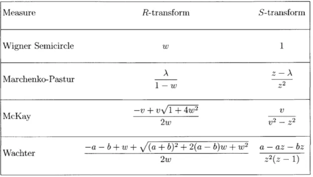
27rx(1 - x) a, b > 1

These four measures have other representations: As their Cauchy, R, and S trans-forms; as their moments and free cumulants; and as their Jacobi parameters and orthogonal polynomial sequences. In fact, their Jacobi parameters (ai,# 4)g0 have

the property that they are "bordered Toeplitz," Ce = a2 an =-- and

#1 = /32 = - - - = n = - - . This motivates the two parts of Chapter 4:

1. We tabulate in one place key properties of the four laws, not all of which can

be found in the literature. These sections are expository, with the exception of the as-of-yet unpublished Wachter moments, and the McKay and Wachter law Jacobi parameters and free cumulants.

2. We describe a new algorithm to exploit the Toeplitz-with-length-k boundary structure. In particular, we show how practical it is to approximate distribu-tions with incomplete information using distribudistribu-tions having nearly-Toeplitz encodings. We can use the theory of Cauchy transforms to go from the first batch of moments or Jacobi parameters of an analytic, compactly-supported distribution to a fine discretization thereof which can be used computationally. Studies of nearly Toeplitz matrices in random matrix theory have been pioneered

by Anshelevich

[2,

3]. Other laws may be characterized as being asymptotically

Toeplitz or numerically Toeplitz fairly quickly, such as the limiting histogram of the eigenvalues of (X//m

+

plI)'(X/-ij + MI), where X is m x n, n is 0(m), and m - oc. Figure 4-3 shows that its histogram can be reconstructed from its first batch of Jacobi parameters. Figure 4-2 shows distributions recovered from random first batches of Jacobi parameters. Figure 4-4 shows the normal distribution - which is not compactly-supported -reasonably well recovered from its first 10 or 20 moments.

Chapter

2

A Matrix Model for the -Wishart

Ensemble

2.1

Introduction

The goal of this chapter is to prove that a random matrix Z has eig(ZtZ) distributed

with pdf equal to the O-ensemble below:

A D

c2 A(A) -oFo()

13 = T

1)dA.

Z's singular values are said to be the VAi. Z is defined by the recursion in the box,

if n is a positive integer and m a real greater than n - 1.

Beta-Wishart (Recursive) Model, W() (D, m, n)

where {rTi, . W(D, m, 1)

rn- 1 )( Lin',n

X(m-n+1)3Dnn ]

.Tn1} are the singular values of W(O)(D.:n_1,1.:n_, m, n - 1), base case

The singular values of WO) (D, m, n) are the singular values of Z.

The critical aspect of the proof is changing variables from the Ti's and x D1n2's to

the singular values of Z and the bottom row of its eigenvector matrix, q. This requires the derivation of a Jacobian between the two sets of variables. In addition, to complete the recursion, a theorem about Jack polynomials is needed. It is originally due to [54] in a different form, the proof in this thesis is due to Praveen Venkataramana. Let q be the surface area measure of the first quadrant of the n-sphere. The theorem is:

C)(A) q-2 1Cf )((I - qqt)A)dq.

The Jack polynomial Cf is defined in Section 2.4.

For completeness we also include the distributions of the extreme eigenvalues, which are due to [19], and we check them with the mhg software from [43].

2.2

Arrow and Broken-Arrow Matrix Jacobians

Define the (symmetric) Arrow Matrix

di Ci

A=

dn-_{1 Cn-1}

C 1 .. Cn-1 Cn

Let its eigenvalues be A,.. . , An. Let q be the last row of its eigenvector matrix, i.e.

q contains the n-th element of each eigenvector. q is by convention in the positive

Define the broken arrow matrix B by

Let its singular values singular vector matrix, the positive quadrant.

Define dq to be the

a,

0 ... 0

be -1,.. . , U, and let q contain the bottom row of its right

i.e. A = BtB, BtB is an arrow matrix. q is by convention in

surface-area element on the sphere in R .

Lemma 1. For an arrow matrix A, let f be the unique map f : (c, d) - (q, A). The

Jacobian of f satisfies:

dqdA = -* dcdd.

1 ci The proof is after Lemma 3.

Lemma 2. For a broken arrow matrix B, let g be the unique map g: (a, b) - (q, or).

The Jacobian of g satisfies:

dqdu = 1 -qi .dadb. f1=1 ai

The proof is after Lemma 3.

Lemma 3. If all elements of a, b, q, - are nonnegative, and b, d, A, o- are ordered, then

f and g are bijections excepting sets of measure zero (if some bi = bj or some di = dj for ij).

Proof. We only prove it for

f;

the g case is similar. We show that

f

is a bijection

using results from Dumitriu and Edelman [12], who in turn cite Parlett [57]. Define an_1

the tridiagonal matrix

7)1 61 0 0

61 2 C2 0

0 0 En-1 ?7n-1

to have eigenvalues dj, ... , d,_₁ and bottom entries of the eigenvector matrix u

(cI,... , cn1)/y, where y = c + -.. - + c2_ 1. Let the whole eigenvector matrix be

U. (d, u) + (6, r) is a bijection[12],

[57]

excepting sets of measure 0. Now we extend the above tridiagonal matrix further and use ~ to indicate similar matrices:

? 1 61 0 0 0

6I T/2 62 0 0

dn_1 Un_17

0 0 6n_1 7n_1 1

0 0 0 1Y C

-(ci,

... ,cn1) e (u, y) is a bijection, as is (ca) + (ca), so we have constructed a

bijection from (ci,... , c_1, cn, di,.. ., dn1) + (cn, y, 1, ), excepting sets of measure

0. (cn, y, I, c) defines a tridiagonal matrix which is in bijection with (q, A) [12], [57].

Hence we have bijected (c, d) ++

(q,

A). The proof that

f

is a bijection is complete. D

Proof of Lemma 1. By Dumitriu and Edelman [12], Lemma 2.9,

dqdA- =

H

dcnd-ydcdTI.

Also by Dumitriu and Edelman [12], Lemma 2.9, n-I dddu = =_ dcdq.

R=1 Ci

Together, n-dqd\ = R =1 q dCndddud-y 1Y R1i u2

The full spherical element is, using -y as the radius, dci -cn = _n-2 dudy. dqdA =q dcdd, which by substitution is dqdA =

I

qj dcdd R=1 ci Hence,

Proof of Lemma 2. Let A = BtB. dA =2

]

-ido-, and since H 1 O- 2

det(BtB) = det(B)2 _{= a2}

_H

1 -1 b , by Lemma 1,

dqd- 2 dcdd.

2nan

Hn1(bici)

The full-matrix Jacobian _,9(a,b)( is

a(c, d) a(a, b) 2a, bn_1 2anI 2a, a, 2b,

The determinant gives dcdd = 2nan Hn b'dadb. So,

u n n-1 b

dqdo- = IM-- fi= dadb

n-1c U n => 1 _dadb. K J ai 2bn-1

an_-2.3

Further Arrow and Broken-Arrow Matrix

Lem-mas

Lemma 4. n-i +1 j=1 2 -1/2 Ck (Ak - d)

Proof. Let v be the eigenvector of A corresponding to Ak. Temporarily fix vn = 1. Using Av = Av, for j < n, v = cj /(Ak - dj). Renormalizing v so that IIvII = 1, we El

get the desired value for v, = qk.

Lemma 5. For a vector x of length 1, define A(x) =H< |xi - xj|. Then,

n-i n

A(A) = A(d)

JJl

Ckj -1.qk

k=1 k=1

Proof. Using a result in Wilkinson [67], the characteristic polynomial of A is:

n p(A) = f(A i=1 n-I - A) = j(di i=1 n-1 A -1 j=1 2 C3 cij - AJ Therefore, for k < n, n p(dk) = J(A - dk) = i=1 n-I

H

(di - dk). i=1,izk

Taking a product on both sides, n n-1

f fj(A - dk)

i=1 k=1

n n-i

p'(Ak) = - (Ai - A) = -f (di

n-1 = ( - )n - )2 c . k=1 - Ak) I + i=1 2 C. (dj - Ak )2} - A) Cn (2.1) (2.2) Also, i=1,ik (2.3) qk -n-1 E j=1

Taking a product on both sides,

n n-1 n n-1 2

-i=1 k=1 n-i i=1 j=1 (d A3

Equating expressions equal to

171

]kJ_- (Ai - dk), we get

n-1 n n-I 2

-A(d)2

_17c

_{= A(A)2 9 1+ ( i}

k=1 i=1 ( j=1

The desired result follows by the previous lemma. E

Lemma 6. For a vector x of length 1, define A 2(x) -717<3 Ix2 - x

\.

The singular

values of B satisfy n-I n A2 (u) - A2_(b)

_H

_Iakbj

171

q;-'. k=1 k=1

Proof. Follows from A = B'B. l

2.4

Jack and Hermite Polynomials

The proof structure of this section, culminating in Theorem 2, is due to my collabo-rator Praveen Venkataramana, as are several of the lemmas.

As in

[141,

if K F k, K = (KI, K2, .. .) is nonnegative, ordered non-increasingly, and

it sums to k. Let a = 2/. Let pc =

>_

Ki(Ki - 1 - (2/a)(i - 1)). We define l(K)

to be the number of nonzero elements of K. We say that A < K in "lexicographic ordering" if for the largest integer j such that pi = Ki for all i < j, we have pIj < Kj. Definition 1. As in Dumitriu, Edelman and Shuman [141, we define the Jack

poly-nomial of a matrix argument, Cfj'(X), as follows: Let x1, ... , xn be the eigenvalues

of X. Cfj3(X) is the only homogeneous polynomial eigenfunction of the Laplace-Beltrami-type operator:

D* = ZX 2 +3

with eigenvalue p' + k(n - 1), having highest order monomial basis

function

in

lexi-cographic ordering (see

[14],

Section 2.4) corresponding to i. In addition,

S

Cf)(X) =trace(X)k.

&4-k,l(i)<n

Lemma 7. If we write Cfi (X) in terms of the eigenvalues x1,. . ., xa, as C

(i(x,

... , Xn),

then C (xi, .(.) . , i_1) = C (xi, ... , xn_₁, 0) if l(s) < n. If l(K) = n, CXn(xi, ... , x- ₁, 0)

0.

Proof. The l(K) = n case follows from a formula in Stanley [63], Propositions 5.1 and

5.5 that only applies if K, > 0,

Cfj)(X) oc det(X)C _1,.

If rn = 0, from Koev [43, (3.8)], C,(j (xi, ... , x,-1) = C(3) (xi, ... , xn_1, 0). E

Definition 2. The Hermite Polynomials (of a matrix argument) are a basis for the

space of symmetric multivariate polynomials over eigenvalues x1,... , x, of X which

are related to the Jack polynomials by (Dumitriu, Edelman, and Shuman

[14J,

page

17)

H()(X) = c - O.

where o- C r means for each i, o- < rj, and the coefficicents c13 are given by (Du-mitriu, Edelman, and Shuman [14], page 17). Since Jack polynomials are homoge-neous, that means

HO)(X) oc C()(X) + L.O.T.

Furthermore, by (Dumitriu, Edelman, and Shuman /14], page 16), the Hermite Poly-nomials are orthogonal with respect to the measure

exp(4 2

_f

_{x - l}

Lemma 8. Let

[I C1 Cl

A (p, c) =

Pn-1 Cn_1 Cf-1

C1 ... Cn-I C j C₁ ... Cn-1 Cn

and let for l(Q) < n, n-1

Q(P, cn) = 4c_ 1 _{H O)(A(_, c)) exp(-c'-- - c_}

1)dc .. dc2_.

i=1

Q

is a symmetric polynomial in p with leading term proportional to H 3(M) plus

terms of order strictly less than i|.

Proof. If we exchange two ci's, i < n, and the corresponding pi's, A(, c) has the same

eigenvalues, so HfjO(A(y, c)) is unchanged. So, we can prove Q(P, cn) is symmetric in p by swapping two pi's, and seeing that the integral is invariant over swapping the

corresponding ci's.

Now since H )(A(p, c)) is a symmetric polynomial in the eigenvalues of A(p, c),

we can write it in the power-sum basis, i.e. it is in the ring generated by t, =

AP + - + AP, for p = 0, 1, 2,3,.. ., if A,,... , An are the eigenvalues of A(p, c). But tp = trace(A(p, c)P), so it is a polynomial in p and c,

H j) (A(p, c)) = ypi,(p)c'c"1 . .. ci[_1. 20 Ei,..,En_1>O

Its order in p and c must be jrj, the same as its order in A. Integrating, it follows that

Q(P, cn) = pE([t)ciMe,

for constants M. Since deg(Hj3 (A(y, c))) = I'i, deg(pi, (y)) < Ir - - i. Writing

Q(1,

cn) = M6POd(P) + pi,E(1p)ci-Mc, (i,E)#(O,5)

we see that the summation has degree at most Hrl - 1 in p only, treating c, as a constant. Now

() M 0

PO 6(p) = Hr Hja(p) + r(p),

0 0

where r(p) has degree at most Jr - 1. This follows from the expansion of H/j3 in

Jack polynomials in Definition 2 and the fact about Jack polynomials in Lemma 7.

The new lemma follows. EI

Lemma 9. Let the arrow matrix below have eigenvalues in A = diag(A1,..., An) and

have q be the last row of its eigenvector matrix, i.e. q contains the n-th element of each eigenvector, 1k c1 ci M A(A, q) /Tn-I Cn-1 Cn-1 L C1 cnI c j c1 ... - 1 cn

By Lemma 3 this is a well-defined map except on a set of measure zero. Then, for U(X) a symmetric homogeneous polynomial of degree k in the eigenvalues of X,

n

V(A)= Jf q,-U(M)dq

is a symmetric homogeneous polynomial of degree k in A1,..., An.

Proof. Let en be the column vector that is 0 everywhere except in the last entry, which

matrix of A(A, q) is

Q,

so must

Q

t(I - ene')QAQt(I - ese')Q

have those eigenvalues. But this is

(I - qqt)A(I - qqt).

So

U(M) = U(eig((I - qqt)A(I - qqt))\{O}).

It is well known that we can write U(M) in the power-sum ring, U(M) is made of

sums and products of functions of the form pp, + - - -

+

_ where p is a positive

integer. Therefore, the RHS is made of functions of the form

p+- -, + OP = trace(((I - qqt)A(I - qqt))P),

which if U(M) is order k in the pi's, must be order k in the Ai's. So V(A) is a polynomial of order k in the A's. Switching A1 and A2 and also qi and q2 leaves

J

q U(eig((I - qq')A(I - qq'))\{0})dq

invariant, so V(A) is symmetric.

Theorem 2 is a new theorem about Jack polynomials.

Theorem 2. Let the arrow matrix below have eigenvalues in A = diag(A,,..., A,)

and have q be the last row of its eigenvector matrix, i.e. q contains the n-th element

of each eigenvector,

Cl

By Lemma 3 this is a well-defined map except on a set of measure zero. a partition r,, l(r;) < n, and q on the first quadrant of the unit sphere,

Cl$;I) (A) cx -n Then, if for Proof. Define ,n q 77(0)J(A) =q- H(3)(M)dq. i=1

This is a symmetric polynomial in n variables (Lemma 9). Thus it can be expanded in Hermite polynomials with max order r (Lemma 9):

(e) (A) =C(rK('), rK)H(")(A),

,~(K)O)

where Isj = /-i1 + r2 + + rS(,). Using orthogonality, from the previous definition of

Hermite Polynomials,

/Anj

AERn/

qf-x eqf-xp(- trace(A2))

2 n I Ai - Aj[dqdA.

Using Lemmas 1 and 3,

A(A, q) = Cl k2n-I Cn-1 Cl M cn-1 ... Cn-1 Cn Cl Cn_1 Cn q 1Hn(3)(M)H )(A) H,()3)(M)HL (" (A) c(r,(O) r') OC C(rO),I r) OC

x exp(--trace( 2 A 2_{)) l - I dydc.} i- ci Using Lemma 6, x exp(- trace(A2 )) 2 HN(' (M) H (")(A)

Hj

I1j - yjdpdc,₁ i:Ai and by substitution c(r 0), I's) c

lu

-

Hsi

'

x exp(- ₂trace(A(A, q)2))

QC,

c(Y ) = _C 1 _{H o0(A(A, q)) exp(-c - - c_1 )dci -1}

-l-Q(p,

c,) is a symmetric polynomial in p (Lemma 8). Furthermore, by Lemma 8,

Q(p,

cn) oc H) (M) + L.O.T.,

where the Lower Order Terms are of lower order than JK(0) and are symmetric poly-nomials. Hence they can be written in a basis of lower order Hermite Polynomials, and as c(i(0), rI) cJ H) (M)Q(pt, cn) x

H

itj - P| 1texp (C itj we have by orthogonality c(r(0),

,)

c 6(r0), r), Jc c(r(0), iK) cX Define

S-pdpdc

+ p+_+ pi) dpdc, (M)HAf " (A (A,7 q))

where 6 is the Dirac Delta. So

r01 (A) Jf q -H( (M)dq

By Lemma 9, coupled with Definition 2, C (A) cx f

i=1

oc H0)(A).

q- Cj) (M)dq.

Corollary 1. Finding the proportionality constant: For l(K) < n,

C (A) = (In)

2n- F(no/2)

17(,3/2)n

J

q

1_{C)((I - qq}t_)A)dq.

Proof. By Theorem 2 with Equation (2.4) (in the proof of Lemma 9),

qI C')(eig((I - qqt)A(I

which by Lemma 7 and properties of matrices is

Cr ( A) oc

Now to find the proportionality constant. Let A = I, and let cp proportionality.

CK( (In) = C -

q1-be the constant of

- C) (I - qq jdq.

Since I - qqt is a projection, we can replace the term in the integral by Cn)(In1), which can be moved out. So

c<(') (I=)

(

qftldq El - qqt)) - {O})dq, 1C(1)((I - qqt) A)dq. Cr(3)(A) ocx , n fl q -i=1

q -idq 2 f~ 'rnOIerV 2_d , n

1d

dr qI31 1(n/3/2) J F(r F(T F(n F(r 2n--~ 2

f f

jfrq _{')OI-1 (rn-ldrdq)} 0/2) 2 n - x -/2) X e xdx 2

(00

n31~~

/3/2)

_jo

_{xl exJ} 2 F(_/2)_ n 0/2) 2J (0/2)n 117(no/2)' and the corollary follows.

Corollary 2. The Jack polynomials can be defined recursively using Corollary 1 and

two results in the compilation [411.

Proof. By Stanley [63], Proposition 4.2, the Jack polynomial of one variable under

the J normalization is

(l') (A,) = An (1 + (2/3)) ... (1 + (K1 - 1)(2/3)).

There exists another recursion for Jack polynomials under the J normalization:

n

Jr3)(A) = det(A)J(-1,._..,_l) J(n - i + 1 + (2/#3)(ni - 1)),

if ru > 0. Note that if rIn > 0 we can use the above formula to reduce the size of , in a recursive expression for a Jack polynomial, and if Kn = 0 we can use Corollary 1 to

reduce the number of variables in a recursive expression for a Jack polynomial. Using those facts together and the conversion between C and J normalizations in [14], we

can define all Jack polynomials. E

2.5

Hypergeometric Functions

Definition 3. We define the hypergeometric

function

of two matrix arguments and

parameter 3, oFo3(X, Y), for n x n matrices X and Y, by

00 oFo(3X, Y) =

k=O i&'k,l(r)<n

Cf(j (X)Cfj (Y) k!Cfj3 (I)

as in Koev and Edelman

[43].

It is efficiently calculated using the

in Koev and Edelman

[43],

mhg, which is available online [42].

polynomials under the C normalization, r H k means that r is

integer k, so 1 ;> r12 > ... > 0 have |jr= k = x1+ 2+ --- = k.

software described The C's are Jack a partition of the

Lemma 10.

0FO ( (X, Y) = exp (s - trace(X)) oFo (3)(X, Y - sI).

Proof. The claim holds for s = 1 by Baker and Forrester [4]. Now, using that fact

with the homogeneity of Jack polynomials,

oFo()(X, Y - sI) = oFo()(X, s((1/s)Y - I)) = oFo('3)(sX, (1/s)Y - I)

exp (s -trace(X)) oFo(') (sX, (1/s)Y) = exp (s -trace(X)) oFo(' (X, Y).

Definition 4. We define the generalized Pochhammer symbol to be, for a partition

K = ('I, . ,K)

(a =riri a - 2

)(3 i=1 j=1 ₂

Definition 5. As in Koev and Edelman

[43],

we define the hypergeometric function

1F1 to be

00

(a),3 C.,()C (Y

iF1 (a;b;X,Y) = () C !(X)C()(Y)

The best software available to compute this function numerically is described in Koev and Edelman [43], mhg.

Definition 6. We define the generalized Gamma function to be

n

F($)(c) = n(n-1),3/4 f -(c - (i - 1)3/2)

for !R(c) > (n - 1)3/2.

2.6

The -Wishart ensemble, and its Spectral

Dis-tribution

The ,3-Wishart ensemble for m x n matrices is defined iteratively; we derive the m x n case from the m x (n - 1) case.

Definition 7. We assume n is a positive integer and m is a real greater than n - 1.

Let D be a positive-definite diagonal n x n matrix. For n = 1, the 43- Wishart ensemble

is

Xm,31/2_1,1

0 Z=,

0

with n - 1 zeros, where X-i3 represents a random positive real that is x-distributed with m/3 degrees of freedom. For n > 1, the 0- Wishart ensemble with positive-definite

diagonal n x n covariance matrix D is defined as follows: Let TI, ... , r_₁ be one

draw of the singular values of the m x (n - 1) /3-Wishart ensemble with covariance

Dl:(n-1),1:(n-1). Define the matrix Z by

T= 1/2

n-- X Dn,n₃

1/2

All the X-distributed random variables are independent. Let o,. . ., on be the singular

values of Z. They are one draw of the singular values of the mxn /3-Wishart ensemble,

completing the recursion. Ai = a are the eigenvalues of the 3-Wishart ensemble.

Theorem 3. Let E = diag(o-1, ... , o-), oi > o-2 > ... > o-n. The singular values of

the 0- Wishart ensemble with covariance D are distributed by a pdf proportional to

det(D) -mo/2 ( m--n+I),--1A2(,,)O oFo(O) -E2,I D-1 do-.

It follows from a simple change of variables that the ordered Ai 's are distributed as

CW' det(D)-m// 2

-A2 lA(A)OoFo-3) A, D-) dA.

Proof. First we need to check the n = 1 case: the one singular value a- is distributed

as -1 = 1D which has pdf proportional to

exp

(,

=D,

₁ dcri.

Di -m/2 .mno-1 ₂ I1 al

We use the fact that

OF o(O) - a , D -1 = F o ( ) --2 D 1,1

The first equality comes from the expansion of OFO in terms of Jack polynomials and the fact that Jack polynomials are homogeneous, see the definition of Jack polyno-mials and OFO in this paper, the second comes from (2.1) in Koev [41], or in Forrester

[28]. We use that oFo"(X, I) = oFo()(X), by definition [43].

Now we assume n > 1. Let

1/2

rn- XpDn,n T_ a,

1/2

so the ai's are X-distributed with different parameters. By hypothesis, the Ti's are a -Wishart draw. Therefore, the ai's and the Ti's are assumed to have joint distribution proportional to n- + det(nm// 2

JfJ

(m-n±2)/3-- lA(T13F( i=1 1 exp

(

(

2D 12 -- T I D-1 2 1:n

where T = diag(i, ... , Tn_1). Using Lemmas 2 and 3, we can change variables to

n- 1F det(D)m!rn3_/2

fI

_Ti~mn±) 3 -A2(),Fo( i=1 ai) a m-n+l)-l exp

k\2Dn,n

-) T2,D _

Using Lemma 6 this becomes:

n-1

det(D)-m3/2

J-

(m-i=1

x exp -j

flnfl

Using properties of determinants this becomes:

n 2

det(D)m!3/ Im~) 3 A() 3 F() (_2 T 1 D1:

1n,n x exp

n

X21 _q13

To complete the induction, we need to prove

1 q 1,1:n 1) 4 dadr, 1,1:n 1) - dadq. 1,1:n-1) a,)f q' 'do-dq i 1 1,1:n 1) 1 d1odq. oFo)

(

- E2 , D a ) a m-n+10m n+1)O-1 2 (a)oF 3 (- T2, D-1 e-Il 12/(2Dn,n) Fo() - T2, D- dq.

We can reduce this expression using Ia| 2 +

Z

=

E

₁ or that it suffices to show

exp (trace(E2_{)/(2Dn,n)) OFO()}

(

2 , D-1)

oC

1

q-1 exp (trace(T2_{)/ (nT2,}

D-or moving some constants and signs around,

exp

((-1/Dn,n)trace(-

E2 /2)) OFO(")

(

2

D-or using Lemma 10,

oFo 2, DDE2

oc

nJ

We will prove this expression termwise using the expansion of OFO into infinitely many Jack polynomials. The (k, r,) term on the right hand side is

fn

IC

K3)

T

-1)

I

- n~ In 1) dq,

where , - k and l(K) < n. The (k, K) term on the left hand side is

Cro) D-1

-

_{In_}

where ' - k and I(K) < n. If l(K) =n, the term is 0 by Lemma 7, so either it has a

corresponding term on the right hand side or it is zero. Hence, using Lemma 7 again

it suffices to show that for l(r,) < n,

C$,) (y 2)

iiq

-1C3) (T 2

)dq.

.1)1:n-1

)

dq,

(2Dn,n)) OFO(

)

oc q exp ((- 1/ (Dn,n)) trace( -T 2/2)) oFo(O) IT 2, ID

I Dn' n .1 q -1 oFo(") IT 2, D-1 _{- ~} -In_ 1 ) dq. Cro) D C o) -. ),1:(n1))dq,

This follows by Theorem 2, and the proof of Theorem 3 is complete. 0

Corollary 3. The normalization constant, for A, > A2 > - > An:

OW- 1

m,n

where

2mno/2 pF~) (m3/2)F$) (n/3/2)

"~ 7 rn(n-1)0/2 F(0/2)n

Proof. We have used the convention that elements of D do not move through oc, so

we may assume D is the identity. Using OFO('3)(-A/2, I) - exp (-trace(A)/2), (Koev [411, (2.1)), the model becomes the /-Laguerre model studied in Forrester [25]. E

Corollary 4. Using Definition 6 of the generalized Gamma, the distribution of Amax

for the 43-Wishart ensemble with general covariance in diagonal D, P(Amax < x), is:

'n)(I + (n - 1)0/2) det mD 1F M ; +n - +1; xD-.

r,)(1) +(m + n - 1)0/2) 2 2 2

Proof. See page 14 of Koev [41], Theorem 6.1. A factor of / is lost due to differences in nomenclature. The best software to calculate this is described in Koev and Edelman [43], mhg. Convergence is improved using formula (2.6) in Koev [41]. El Corollary 5. The distribution of Amin for the 3- Wishart ensemble with general co-variance in diagonal D, P(Amin < x), is:

nt~ Q)(xD--1/2)

1 - exp (trace(-xD-1/2)) k(

E k!

k=O &1k,,1<t

It is only valid when t = (m - n + 1)0/2 - 1 is a nonnegative integer.

Proof. See page 14-15 of Koev [41], Theorem 6.1. A factor of

4

is lost due to

differ-ences in nomenclature. The best software to calculate this is described in Koev and

Edelman [43], mhg. D

[41] Theorem 6.2 gives a formula for the distribution of the trace of the 3-Wishart ensemble.

0.9- 0.8- 0.7- 0.6- 0.5- 0.4- 0.3- 0.2- 0.1-0 0 20 40 60 80 100 120

Figure 2-1: The line is the empirical cdf created from many draws of the maximum

eigenvalue of the -Wishart ensemble, with m = 4, n = 4, ,3 = 2.5, and D =

diag(1.1, 1.2, 1.4, 1.8). The x's are the analytically derived values of the cdf using Corollary 4 and mhg.

The Figures 2-1, 2-2, 2-3, and 2-4 demonstrate the correctness of Corollaries 4 and 5, which are derived from Theorem 3.

2.7

The

#-Wishart

Ensemble and Free Probability

Given the eigenvalue distributions of two large random matrices, free probability allows one to analytically compute the eigenvalue distributions of the sum and product of those matrices (a good summary is Nadakuditi and Edelman [59]). In particular, we would like to compute the eigenvalue histogram for XtXD/(m), where X is a tall matrix of standard normal reals, complexes, quaternions, or Ghosts, and D is a positive definite diagonal matrix drawn from a prior. Dumitriu [13] proves that for the

D = I and 0 = 1, 2,4 case, the answer is the Marcenko-Pastur law, invariant over 6.

So it is reasonable to assume that the value of 3 does not figure into hist(eig(XtXD)),

where D is random.

We use the methods of Olver and Nadakuditi [56] to analytically compute the product of the Marcenko-Pastur distribution for m/n -- + 10 and variance 1 with the Semicircle distribution of width 2f2/ centered at 3. Figure 2-5 demonstrates that

0.9- 0.8- 0.7- 0.6- 0.5- 0.4- 0.3-0.2 -0.1 -0 0 10 20 30 40 50 60 70

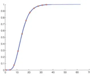
Figure 2-2: The line is the empirical cdf created from many draws of the maximum eigenvalue of the 3-Wishart ensemble, with m = 6, n = 4, / = 0.75, and D =

diag(1.1, 1.2, 1.4, 1.8). The x's are the analytically derived values of the cdf using

Corollary 4 and mhg. 1 -0 0.9- 0.8- 0.7- 0.6- 0.5- 0.4- 0.3- 0.2- 0.1-0 5 10 15 20 25

Figure 2-3: The line is the empirical cdf created from many draws of the

mini-mum eigenvalue of the /-Wishart ensemble, with m = 4, n = 3, 3 = 5, and

D = diag(1.1, 1.2, 1.4). The x's are the analytically derived values of the cdf

0.9- 0.8- 0.7- 0.6-5 and mlig 0.4 -0.3 -0.2 0.1 0 0 8 1'0 12 14

Figure 2-4: The line is the empirical cdf created from many draws of the minimum eigenvalue of the O-Wishart ensemble, with m = 7, n = 4, 3 = 0.5, and D =

diag (1, 2, 3, 4). The x's are the analytically derived values of the cdf using Corollary

5 and mhg.

the histogram of 1000 draws of XtXD/(m3) for m = 1000, n = 100, and / = 3,

represented as a bar graph, is equal to the analytically computed red line. The /-Wishart distribution allows us to draw the eigenvalues of XtXD/(mO), even if we cannot sample the entries of the matrix for 3 = 3.

2.8

Acknowledgements

We acknowledge the support of National Science Foundation through grants SOLAR Grant No. 1035400, DMS-1035400, and DMS-1016086. Alexander Dubbs was funded

by the NSF GRFP.

We also acknowledge the partial support by the Woodward Fund for Applied Mathematics at San Jose State University, a gift from the estate of Mrs. Marie Wood-ward in memory of her son, Henry Tynham WoodWood-ward. He was an alumnus of the Mathematics Department at San Jose State University and worked with research groups at NASA Ames.

0.35 0.3 0.25 0.2 0.15 0.1 0.05 0 1 2 3 4 5 6 7

Figure 2-5: The analytical product of the Semicircle and Marcenko-Pastur laws is the red line, the histogram is 1000 draws of the ,-Wishart (3 = 3) with covariance drawn

Chapter 3

A Matrix Model for the

#-MANOVA

Ensemble

3.1

Introduction

Recall from the thesis introduction, that:

Beta-MANOVA Model Pseudocode

Function C := BetaMANOVA(m, n, p, #, Q)

A := BetaWishart(m, n , 3 _Q2

)

M :=BetaWishart (p, n , 13,

A-1-C := (M + I)-2

Our main theorem is the joint distribution of the elements of C,

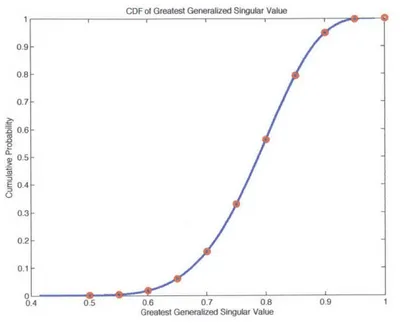
Theorem 4. The distribution of the generalized singular values diag(C) = (c1, ... ,Cn)

c1 > c2 > ... > cn, generated by the above algorithm for m, p > n is equal to:

2nldi3) nnI

2 +p" n det(Q)P' 1 7 cl (p-n+l)/-1 -_7J(i - 3)1 c - C |#

m,n p,n i=1 i=1 i<j

x 1Fo) ( -2P 3; C2(C2 - I)

where 1Fj()) and IC$ 2 are defined in the upcoming section, Preliminaries.

We also find the distributions of the largest generalized singular value in certain cases, generalizing Dumitriu and Koev's results in on the Jacobi ensemble in [15].

Theorem 5. If t = (m - n + 1)0/2 - 1 E Z>O,

P(ci < x) = detr 2Q2 2_{)I+ x2Q2)1)92}

n t (

x

I

(pO/2)f)C3)

((1

- x2)((1 - x2_{)I + x}2_Q2 _-1

₎

_{, (3.1)}

k=O K1-kK<t

where the Jack polynomial C and Pochhammer symbol (.) ) are defined in the

upcoming section, Preliminaries.

The following section contains preliminaries to the proofs of Theorems 4 and 5 in the general 1 case. Most important are several propositions concerning Jack poly-nomials and hypergeometric functions. Proposition 1 was conjectured by Macdonald [47] and proved by Baker and Forrester [4], Proposition 3 is due to Kaneko, in a paper containing many results on Selberg-type integrals [39], and the other propositions are found in [26, pp. 593-596].

3.2

Preliminaries

Definition 8. We define the generalized gamma function to be

F$()(c) - 7nCn-i34

J

F(c - (i - 1)13/2) for W(c) > (n - 1)1/2. Definition 9. 2mn /2 p() (m/3/2) IF) (n1/2) rmn n(n-1)0/2 _F(13/2)n Definition 10.

A(A) =

f(Ai

- Aj).

If X is a diagonal matrix,

A(X) H IXi,i - X, L.

i<j

As in [141, if H F k, K (K1, K2,... , Kn) is nonnegative, ordered non-increasingly,

and it sums to k. Let a = 2/3. Let po = n _1 j(rj - 1 - (2/a)(i - 1)). We define

l() to be the number of nonzero elements of K. We say that p < K in "lexicographic

ordering" if for the largest integer j such that pi = Ki for all i < j, we have yj < Kj.

Definition 11. We define the Jack polynomial of a matrix argument, Cfi'(X), (see,

for example, [14]) as follows: Let x1,... ,x, be the eigenvalues of X. CK (X) is the

only homogeneous polynomial eigenfunction of the Laplace-Beltrami-type operator:

n9

D* = x2 +13.

-n i j- 1 i54j~n E T1 xj - xi'

with eigenvalue pa + k(n - 1), having highest order monomial basis function in

lex-icographic ordering (see Dumitriu, Edelman, Shuman, Section 2.4) corresponding to

K. In addition,

S

Cl)(X) =trace(X)k.

Kk,l(K) n

Definition 12. We define the generalized Pochhammer symbol to be, for a partition

K = (K1, . . ., Ki)

(a)() =

fj

( a - - +13 - 1).

i=1 j=1 )

Definition 13. As in Koev and Edelman [43], we define the hypergeometric function SF(O to be

00 (al)13 ... (ap)l C,( 3(X)C,(' (Y)

F, na; X ,k (b )K(' -... (bq) K$ k!C

f3

(I)

The best software available to compute this function numerically is described in Koev

We will also need several theorems from the literature about integrals of Jack polynomials and hypergeometric functions.

The first was conjectured by MacDonald [47] and proved by Baker and Forrester

([4],

(6.1)) with the wrong constant. The correct constant is found using Special Functions [1, p. 406] (Corollary 8.2.2):

Proposition 1. Let Y be a diagonal matrix.

"F" (a + (n - 1)>/2 + 1)(a + (n - 1)3/2 + 1) C3)(Y-1) y a+(n-l)/ 2

+1 OF0,

(-X,Y)

IX aCj) (X)|A(X |dX,

where c 3

) = -n(n-1)3/4n!F(3/2) In I F(i/3/2).

From [26, p.593],

Proposition 2. If X < I is diagonal,

1Fo( ; X) = 1I - XI.I(a;

Kaneko, Corollary 2 [39]:

Proposition 3. Let K = (I,. .. , n) be nonincreasing and X be diagonal. Let a,b >

-1 and /3> 0.

C(j (X)A(X),3 [xa(I - Xi)b] dX

O<X<I 1

C

)

F(i/2 + i)F(h2 + a + (//2)(n - i) + 1)F(b + (#/2)(n - i) + 1)

=~ f Cr() ((0/2) + 1)F(Ki + a + b + (0/2)(2n - Z'- 1) + 2)

From [26, p. 595],

Proposition 4. Let X be diagonal,

2FI$')(a, b; c; X) = 2FI))(c - a, b; c; -X(I - X )1)1I - X|-b

From [26, p. 596],

Proposition 5. If X is n x n diagonal and a or b is a nonpositive integer,

2F/)(a, b; c; X) -From [26, p. 5941, Proposition 6. 2FP)(a, b; C; I)2Fo)(a, b; a + b + 1 + (n - 1)3/2 - c; I - X). 2FIP)(a, b; c; I)

3.3

Main Theorems

Proof of Theorem 4. Let m, p > n.

0) (c) ) (c - a - b) r) (c - a)F 13(c - b)

We will draw M by drawing A ~ P(A) = BetaWishart(m, n , Q2_{), and compute M by drawing}

M ~ P(MIA) = BetaWishart(p, n, /3, A- 1)-1.

The distribution of M is f P(MIA)P(A)dA. Then we will compute C by C = (M +

I)-2. We use the convention that eigenvalues and generalized singular values are

unordered. By the paper [10], the BetaWishart described in the introduction, we sample the diagonal A from

P(A) - det(A MI n!/m ,n n A+1 2t + , 1 _A-

_Aj

3_oFo('3₎ 2mn,/2 m,n ,n(n-1)0/2 p$()(m3/2)P F(nl3/2)

Likewise, by inverting the answer to the [10] BetaWishart described in the intro-duction, we can sample diagonal M from

(

1