Bottomless continuous-time continuous-state two-machine transfer line

Bottomless Continuous-Time Continuous-State Two-Machine Transfer Line By Xiaoliang Yao B.S. Industrial Engineering B.S. Applied Mathematics B.A. Economics B.A. Chinese Language

B.B.A. Finance and Operations Management University of Massachusetts Amherst, 2011

M.S. Operations Research Columbia University, 2013

Submitted to the System Design and Management Program and the Department of Mechanical Engineering in Partial Fulfillment of the Requirements for the Degrees

of

Master of Science in Engineering and Management and Master of Science in Mechanical Engineering

at the

Massachusetts Institute of Technology

June 2018

Q 2018 Massachusetts Institute of Technology. All rights reserved

Signature of Author...Signature

redacted

System Design a d n aagement Program Department 1echanical Engineering

Signature redacted

Senior Research Scientist,

Signatur

JUN 2

0

2018

LIBRARIES

red acted

. ...

Joan Rubin ector, System Design and Management

Signature redacted

Bottomless Continuous-Time Continuous-State Two-Machine

Transfer Line

by

Xiaoliang Yao

Submitted to the MIT Sloan School of Management and the Department of Mechanical Engineering

on May 25, 2018, in partial fulfillment of the requirements for the degrees of

Masters of Science in Engineering and Management and

Masters of Science in Mechanical Engineering

Abstract

In this thesis, we first present a model and analysis of a two-machine continuous-time, continuous-material, mixed-state transfer line with an allowance for negative inventory. The production line consists of two-machines separated by a storage area with a maximum storage level N, and minimum storage level -oc. In other words, inventory level is allowed to be negative, while the first machine can be blocked, the second machine is never starved. This new model is based on unreliable machines, to represent a system of stochastic supply and demand with the possibility of backlog. Thesis Supervisor: Stanley B. Gershwin

Acknowledgments

This thesis is dedicated to my mother, for her emotional support and her gentle reminders to focus on what's important in life; to my Wife Katy for putting up with my never-ending academic responsibilities; to my Brother James for providing me with joy and laughter; and to my Friend Stephen for being there for me whenever I needed support and friendship.

Thanks to Dr. Stanley B. Gershwin for his wisdom and guidance on this thesis; to Dr. Chris Caplice, Dr. Eva Ponce and the CTL for providing me with financial support during my time here at MIT; and to my friends Shruti Banda and Carlos Damas for having faith in my ability.

Contents

1 Introduction 11

1.1 Problem Statement . . . . 11

1.2 Literature Review . . . . 12

1.3 Thesis Outline. . . . . 13

2 Bottomless Buffer Continuous Two-Machine Line 15 2.1 Model assumptions, notations, terminology, conventions and relations to previous work . . . . 16 2.2 Performance Parameters . . . . 17 2.3 Transition Equations . . . . 19 3 Solution Technique 23 3.1 C ase 1: P I = 2 . . . . . . . . 24 3.2 Case 2: Pi1 i P2 ...... 26 3.2.1 P1 > p2 . . . . . . . . 26 3.2.2 p 2 > P1 . . . . 27 3.2.3 Production Rates . . . . 28

3.3 Numerical results and interpretation . . . . 30

3.3.2 Varying A2. . . . . . . 3

4 Optimization 37 4.1 Form ulation . . . . 37

4.2 Numerical results and interpretation . . . . 40

4.2.1 Unreliable Demand . . . . 40

4.2.2 Reliable Dem and . . . . 44

4.2.3 Key Relationships . . . . 48

5 Conclusion and Future Research 53

A Derivations 55

List of Figures

1-1 Bottomless two-machine line. . . . . 13

3-1 Comparison t of the regular vs bottomless two-machine line as pi is increasing, rl = 0.1, r2 = 0-1, Pi = 0.1, P2 = 0.5,p2= 2 . . . . 30 3-2 Comparison of PA of the regular vs bottomless two-machine line as A,

is increasing, r, = 0.1, r2 = 0.1, Pi = 0-1, P2 = 0.5,,P2 = 2 . . . . 32 3-4 Comparison of PA of the regular vs bottomless two-machine line as P2

is increasing, r1 = 0.1, r2 = 0-1, P1 = 0.1, P2 = 0.5, p1 = 2 . . . . 34

3-3 _{Comparison of t of the regular vs bottomless two-machine line as} 1u2

is increasing, r1 = 0.1,r2 = 0-1,Pi = 0-1,P2 = 0.5, p1 = 2 . . . . 35

4-1 Optimal buffer size given equal surplus and backlog costs and un-reliable demand, pi = 0.8 9 5, P2 = 0.890, g- = 2, g+ = 2, ri/r2 =

0.9,Pi/P2 = 0.01 . . . . . . . . 40 4-2 Optimal buffer size when surplus cost is increased to g+ = 20, p, =

0.895, P2 = 0.890, g_ = 2, g+ = 20, ri/r2 = 0.9, p1/p2 = 0.01 . . . . 42

4-3 Optimal buffer size when surplus cost is increased to g_ = -20,pl =

4-4 Optimal buffer size given reliable demand with equal surplus and backlog cost, pi 0.8 9 5, P2 = 0.890, g = 2,g+ = 2,r_{1 =} 0.9,pi =

0.0 1, P 2 = 0 . . . . 45

4-5 Optimal buffer size given reliable demand with surplus cost increased to g+ 20, pi 0.89 5, P2 = 0.890,g_ = 2, g+ 20, r = 0.9,Pi =

0 .0 1, P 2 = 0 . . . . 46

4-6 Optimal buffer size given reliable demand with backlog cost increased to g_ = -20, pi = 0.8 9 5, P2 = 0.890, g- = 20, g+ = 2, r1 = 0.9,pi =

0.01, P2 = 0 . . . . 47

4-7 Relationship among the surplus cost, backlog cost, optimal cost, op-timal Buffer Size and st, 9 vs N*, i*, E*[g(x)], pi = 0.895, P2 = 0.890

for both graphs . . . . 48 4-8 Behavior of N*, * and E*[g(x)] as the ratio of P' increases at a given

P2

=0.02, i vs N*, , E*[g(x)]. = 0.02 . . . . 51

9g P2 9

Chapter 1

Introduction

1.1

Problem Statement

This thesis presents a model and analysis of a two-machine, single-buffer transfer line as a continuous time, mixed state Markov process. The assumptions on which this model is based are similar to the Continuous Model presented in Gershwin[1]. In general, the machines are allowed to operate at different speeds. In addition, the inventory buffer level is allowed to go from -oc to a maximum storage level N, thus the first machine is sometimes blocked, but the second machine is never starved. As a consequence, the rate at which the first machine fails is affected by storage level, while the rate at which the second machine fails is not. In the optimization section of this paper, this model becomes an extension to the Bielecki & Kumar[9], where our model presents unreliable demand.

1.2

Literature Review

Manufacturing systems have long been a subject of academic research and indus-trial interest. However, most companies rely on heuristics to manage these complex systems, and analytical engineering methods have only reached limited adoption.

The purpose of developing Markov models of two-machine transfer lines is to predict the performance of the line, in the interest of optimizing line design and pro-duction schedule. Two-machine transfer lines with a finite buffer have been studied extensively in the past. Gershwin[1] presented a deterministic-time, discrete material model where the operation time of both machines are equal and the machines have geometric failure and repair processes. Gershwin & Berman[3] described a Markov process model of a finite buffer transfer line which contains machines with expo-nential service, failure and repair processes, and the movement of discrete parts. Gershwin & Schick[2] presented a continuous-time, mixed state process, where the flow of material is treated as though it is a continuous fluid. The assumptions in this model are more flexible than the deterministic model in that the machines can oper-ate at different speeds. Finally, Tan & Gershwin[4] developed a general Markovian two-machine continuous-flow line with a finite buffer. In this model, the machines are allowed to have multiple up and multiple down states associated with their quality characteristics.

These two-machine subsystems can later be treated as building blocks in solving much longer production lines through analytical approximations. Gershwin[6] and Dallery, David & Xie[5] presented decomposition methods for solving long lines with deterministic-time, discrete material, two-machine transfer lines as building blocks. Burman[7] introduced the ADDX algorithm to approximate the performance of long lines with continuous-time, continuous-flow two-machine lines as its building block.

N

M1 B M2

P1, 1r 1P -0 P2,T2,P2

Figure 1-1: Bottomless two-machine line.

Lastly, Colledani & Gershwin[8] presented a decomposition methods for the approx-imation of continuous-flow, multi-stage, general Markovian machine lines.

The purpose of this thesis is to introduce an extension to the continuous-time, continuous-flow, two-machine line, where the buffer has a finite maximum storage limit, but an infinitely negative minimum storage limit. This model is an extension of the work done by Gershwin & Schick[2], where instead the lower limit of the buffer level is 0, it can go to -oo. This new model is based on unreliable machines, to represent a system of stochastic supply and demand with the possibility of backlog.

1.3

Thesis Outline

The paper is organized as follows. Chapter 2 introduces the bottomless-buffer, con-tinuous two-machine line in detail. Chapter 3 presents the solution technique for solving the model presented in Chapter 2. An optimization procedure is introduced in determining the optimal maximum buffer size N including numerical analysis in Chapter 4. Lastly, the conclusion and an outline for future research is described in Chapter 5.

Figure 1-1 shows a continuous time and material two-machine line with a buffer of maximum storage capacity N and minimum capacity -oc.

Chapter 2

Bottomless Buffer Continuous

Two-Machine Line

In this model, the service, repair and failure times for machine Mi are exponentially distributed random variables with parameters piI ri, pi; for i = 1, 2. We will refer to these quantities as the service rate, repair rate and failure rate, respectively. Addi-tionally, let x be the inventory level of the buffer, where -oc < x < N. Negative inventory can be understood as the backlog, especially if M2 is interpreted as

de-mand. Lastly, let ai(t) represent the state of M1 at time t, where ai(t) = 1 means

the machine is operational at time t; ai(t) = 0 means the machine is down at time t.

When a machine is under repair, it stays in that state for a period of time that is exponentially distributed with a mean of 1/ri. Similarly, when a machine is op-erational, M1 will stay operational with an period of time that is exponentially

distributed with a mean of 1/pi, if it is not blocked. Since M2 can never be starved,

it will operate for a period of time that is exponentially distributed with mean 1/P2, until a failure occurs.

Since we defined pi as the speed at which the Mi processes material, buffer B will gain material from MI at a rate of ft_{1 when MI is operational and not blocked,}

until the inventory level reaches maximum capacity N. It loses material to M2 at a rate of p2 when M2 is operational. The net rate of change on the buffer is P/2 - pi, when both machines are operational, M1 is not blocked and the buffer is not full.

Lastly, if Mi is operational for a time interval t, it is assumed that the failure probability of Mi is pi6t, unless x = N and M2 is not operational. In that case M,

is blocked and cannot fail. If x = N and M2 is operational, then failure rate is P ,/'2 when P2 < Ai.

2.1

Model assumptions, notations, terminology,

con-ventions and relations to previous work

During the time interval (t, t + 6t):

When -oc <x<N

1. the change in x is (aip1 - a2/12)6t

2. P(ai(t + 6t) = 1|ai(t) = 0) = rit 3. P(a (t + t) = 0|a (t) = 1) = piot

When x = N

1. the change in x is (alp, - a2[t2)-6t

3. P(cq(t + 6t) = oai(t) = 1 n a2(t) = 0) = 0, since M1 is blocked.

4. P(a1(t + t) = 01ci(t) = 1 n a₂(t) = 1) =p15t, where

b Pill~ P _p= P, I 1 i (2.1) (2.2) (2.3) p = min(PI, A2) b < P, Pi P 5. P(a2(t + 6t) = 0 |a2(t) = 1) = p26t

Equations (2.1) and (2.2) combined describe the failure rate of M1 when x = N.

Since if P2 < pi, M1 is blocked until M2 consumes a part. If 1 < P2, then M will

never be blocked as long as M2 is operational. These assumptions are identical to

those of the original continuous-time, mixed-state process proposed by Gershwin & Schick[2].

2.2

Performance Parameters

Let Ej be the efficiency of Mi, the probability that Mi is operating, defined by

El = P(ai = 1, x < N) _(2.4)

(2.5)

Let P be the production rate of Mi, given by,

Pi = pjE (2.6)

The isolated efficiency ej represents the fraction of time that Mi is operational, and is defined by,

ej =(2.7) ri + pi

The isolated production rate pi, represents the production rate if the machines are never starved or blocked. Since we know that M1 is sometimes blocked, while M2 is

never starved, pi is defined by,

Pi = Pe₁ ; Pi (2.8)

P2 = 2t2e2 P2 (2.9)

Since pi represents the production rate when the system is never starved or blocked, we derive the feasibility following condition,

Pi > P2 (2.10)

This is because if P2 is greater than pi, M2 will always consume inventory faster

than M can replenish, and the system will become infinitely negative, such that no steady state solution can be obtained.

Flow Rate-Idle Time Relationship

The flow rate-idle time relationship is defined as,

P = pP(x < N) (2.11)

P2 = P2 (2.12)

PI = P2 (2.13)

Since pi > P2, _{the system is in steady-state. Consequently, the production rate of}

M1 will always be equal to the production rate of M₂.

2.3

Transition Equations

In the continuous two-machine line, the probability of finding the inventory in a cer-tain interval and both machines in their respective states is made up of a probability density function and a probability mass function. The probability mass function occurs when the inventory level reaches the maximum level N.

Let

f (x, cI, a2, t)6x + O(6x) (2.14)

be the probability of finding the inventory level between x and x + 6x, with Mi in state aj, at time t, when x < N and x + 6x < N.

Let,

P(N, al, a2, t) (2.15) be the probability of finding the inventory level at the maximum, N, with Mi in state aj, at time t.

Intermediate Storage Behavior

By taking the time derivative of the probability density function at the four sets

of machine states, we get the following partial differential equations.

Of _Of

( 1 1) = -(Pi + p2)f (x, 1,1) + (2 - PI) (, 1,+1) + rif (x, 0, 1) + r2f (X, 1, 0) (2.16)

Of

_af

(X,

f

When solving for the steady state probabilities, we will set all time derivatives to 0, and solve the system of partial differential equations with respect to x. The internal behavior of the system is identical to that of the original continuous-time, mixed-state system proposed by Gershwin & Schick[2], the derivations can be found in Gershwin[1].

Boundary Storage Behavior

While the internal behavior of the system can be captured by the probability density function, the probability of finding the system at the boundary, x = N, is represented by Equation (2.15).

By taking the time derivatives of the probability mass functions at the four sets

of machine states, we get the following ordinary differential equations.

d P(N, 0, 0) = -(r ₁ + r2)P(N, 0, 0) (2.20) dt dP(N, 1, 0) = riP(N, 0, 0) - r₂P(N, 1, 0) + p2P(N, 1, 1) + p1

f

{P(N,

If P2 > pi, then P(N, 1, 1) will always be 0, since M2 will consume inventory faster

P(NO , 1) =0 (

The system cannot stay at N since M, is not operational, while M2 will continue to

consume inventory. The boundary behavior of the system, when x = N, is identical

to that of the original continuous-time, mixed-state system proposed by Gershwin & Schick[2], the derivations can be found in Gershwin[1].

Once again, by setting all the time derivatives to 0, and solving the systems of equations, we then obtain the steady state probabilities of the system at the boundary.

Normalization

Now we sum over all of the probability density and mass functions, which is always 1. Thus,

Z1,

al =0 2 = .O

Chapter

₃

Solution Technique

Let the solution of the steady state probability density function assume exponential form. Then Equation (2.14) becomesi,

f (X,) i, a2) = CeXYi 1Y22 (3.1)

By solving Equations (2.16) thru (2.19) and assuming Equation (3.1), we will

result in three parametric equation,

2

Z

1

Gershwin[1] shows that by solving the system of parametric equations, we can

now obtain two solutions to A, Y, Y2 to Equation (3.1). However, for our model, we

will only consider the case when A > 0. If A < 0, then the integral of Equation (3.1) from -oc to N with respect to x will not converge. In this case, Equation (3.1) cannot be a probability density function.

One solution is Y = r (3.5) Pi Y2 = 2 (3.6) P2 A = 0 (3.7)

By eliminating A and Y2, and removing a factor (p1Yi - ri), the parametric

equations reduce to a quadratic equation in Y1:

-(/2 - p1)P1Y12 + [(A2 - pi)(ri + r2) - (P2P1 + P1P2)]Y1 + p2(r1 + r2) = 0 (3.8)

3.1

Case 1:

[I

P1 = P2 is a special case because the quadratic equation (3.8) reduces to a linear equation where Y= Y= - r2 (3.9) P1 +P2 1 1 1 A = -(r1P₂ - r₂Pl)( +

)

the following two equations P(N, 1, 0) = C eAN (r, + r 2) PiTi P(N, 1,1) = C eAN Ti + T2 Pi P1 +P2 (3-11) (3.12)

Note, in this case, the two sets of solutions to the parametric equations, Equations

(3.3) thru (3.4), are the same. Thus, there is only one A to consider. By using

Equation (2.24), we now have the following relationship and C can be then obtained

(3.13)

i

+

ai=O Q2=0

Here A must be greater than 0, otherwise, the integral in converge. If A is non-positive, then the term (TiP2 - r2PI)

be non-positive. That will imply el - e2 is non-positive. violate the feasibility condition that pi > P2.

Equation (2.24) will not in Equation (3.10) must Since p1 = P2, this will

Expected Inventory

The average level of inventory in the system can be expressed as2

C 1

2 = AN(N - )Y2y2 ) 1 + NP(N, ai, a2) a1=0 a2=0

(3.14)

2

3.2

Case 2:

#2

Here the probability density function becomes a summation of two terms. This is due to the two solutions of Y and Y2, when solving the parametric equations.

2

f (x, ai, a2) Z CAeXYg Y2j

j=1

(3.15)

For the same reason as the case 1, the integral in Equation (2.24) will not converge when A, is negative. if Ai is negative, then set C, to 0.

3.2.1 _{/1i > P2}

Probability Distributions

By solving Equations (2.21) and (2.22)

following probability mass functions.

P(N, 1, 1)=

Pi

with Equation (3.15), we can obtain the

2

SCye

When pi > A2, the solution to the parametric equations will yield a positive A as well as a non-positive A '. By setting the coefficient Cj of the non-positive A to 0, one

of the summation terms in Equation (3.15) drops out. Now by invoking Equation

(3.13), the normalizing coefficient can be found.

In the original continuous-time, mixed-state system, the solution to the

para-3_{Many different parameters were tried. In every case, only one A}

metric equations will yield two positive As. Due to the existence of lower boundary conditions. At x = 0, a second equation is available to solve for the second

normal-izing coefficient C2.

Expected Inventory

The average inventory level is given by Equation (3.14), because similar to case

1, there is only one A

3.2.2 [L2 > [L1

Probability Distributions

Here, once again by solving Equations (2.21) and (2.22), the probability mass functions are given by the following expressions.

2

P(N,1,O) = p2 -

Z

F2 j=1

P(N, 1, 1) = 0 (3.19)

Here, to solve for C1 and C2 we will require two equations. We introduce the following relationship.

N-p26t t+6t

-f (x, 0, 1, t + 6t)dx = r₂P(N, 0, 0, s) + pbP(N, 1,1, s)ds (3.20)

N tI

This relationship holds because if at time t, the buffer is full at level (x = N), the

system can only reach the internal state of (x, 0, 1) at time t + 6t, where N - p₂6t <

x < N, from the boundary state (N, 0,0) if M₂ gets repaired, from the boundary

state (N, 1, 1) if M1 goes down or if the system is already in an internal state at time t.

By accounting for the first order terms in Equation (3.20), we have the following expression.

2

f

(3.22)

2 2

f(N, 0, 1) = CjeNY2 0

j=1 a2=1

Now, Equations (2.24) and (3.22) provide two equations and two unknowns, C1 and C2 can now be found.

Expected Inventory

t is simply Equation (3.14) summed over the two coefficients4_.

= TeN(N - _A )1

1Y2j + NP(N, a,, a₂)

j=1 a1=Oca2=0 ( A

(3.23)

3.2.3

Production Rates

The production rate of the system will simply be the production rate of M2, since it

is never starved. From Equation 11, we then know that the production rate is simply

P = p2 (3.24)

The production rate of the first machine can be derived from Equation (2.11).

4_{Derivation similar to Equation (3.14).}

Let Pb be the probability the machine is blocked, then

Pb = 1 -P(x < N) = P(N, 1, 0) + (1 - 112 )P(N, 1, 1) (3.25)

II

This relationship is due to the fact that when the buffer is full and M2 is not

op-erational, M1 is blocked. However, if M2 is operational, then M1 can operate at a

reduced rate if /pi > ip2. If A2 > pi, then recall Equation (2.22), that P(N, 1, 1) = 0.

Now from Equation (2.11), we can establish that

3.3

Numerical results and interpretation

3.3.1

Varying p

.-

Figure 3-1: Comparison t of the regular vs bottomless two-machine line as p1 is

... r --- -... ...r ... .... .... ..7 .... ... ...1---- -0 Regular --~Bottomless -40 20 0 -20 -40 -60 40 --- --- t ma -. 20 0 -20 F -40[ 2.2 A.4 30

Figure 3-1 is a comparison of expected inventory level of the regular two-machine line against the bottomless case. Here, the buffer size is N = 3 in case (a) and

N = 20 in case (b). The numerical results offer a reasonable interpretation. In both figures, the bottomless case tended to converge to the regular case as A, increases, since the system becomes increasingly likely to be full. This convergence happens earlier for N = 20, because x is less likely to be negative with a larger buffer size. However, when p, is small, the bottomless case is highly sensitive and becomes negative quickly. As p1 decreases, the slope of the bottomless curve approaches a

vertical asymptote at p*, where pi = [r _Iri-tpl = p2 = 2r. Lastly, although the two P r2-t-P2

curves tend to converge, the inventory for the bottomless case is always less than the inventory of the regular case. This is because, for the bottomless case, the system has to compensate for all backlog, while there is no backlog in the regular case.

0.9 -0.8 0.7 -0.4 ₁ 0.3t 0.2 0.1 0 , 0.8 1 1.2 1.4 1.6 1.8 2 2.2 2.4 2.8 mu2 (a) Pb vs pi, N = 3 1r *Bottomless 0.9 0.8 0.6 -0.5 -0 0.4-0- eI 0.3 0.2--0.1 -) 0.8 1 1.2 1.A 1.8 1.8 2 2.2 2.4 2.6 mu2 (b) P vs I1, N = 20

Figure 3-2: Comparison of PA of the regular vs bottomless two-machine line as p1 is increasing, r1 = 0.1, r2 = 0-1, P1 = 0-1, P2 = 0.5, pL2 = 2

In Figure 3-2, We compare Pb, derived in Equation (3.25), between the regular and the bottomless cases. As one may expect, Pb will increase as p, increases, since

the system is more likely to be at x = N. However, when p1 is small, the difference

between the PA of the two models is large. One can reasonably infer that the system will spend more time with x being negative for the bottomless case than when A, is large. Lastly, Pb is lower for the bottomless case compared to the regular case when

N is small because the system is spending more time at x = N. When N is large,

there is less difference in PA between the two models.

3.3.2 Varying /12

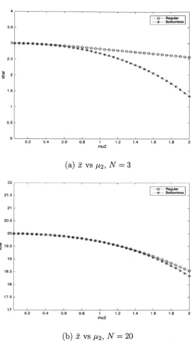
In Figure 3-3, we compare t of the two models as P2 is varied. As expected, the

system starts out near x = N since /u₂ is small. When p₂ becomes large, drops as inventory is increasingly consumed. However, if N is large, the difference between the two models is small, since Pb is smaller, which means that in the bottomless case,

M1 is much less likely to be blocked as compared to when N = 3.

Lastly in Figure 3-4, we compare PA of the two systems as P2 is increasing. PA in this comparison is decreasing almost linearly as p2 is increasing, meaning inventory

consumption is increasing. Thus the buffer is becoming less likely to be full. Once again, when N is small, there is a bigger difference in the system as the bottomless case is less likely to be blocked, since it spends time compensating for backlogs.

0.95 4 '. -otmls 0.9- 0.85-0.75 0.7 0.2 0.4 0.6 0.8 1 1.2 1.4 1.6 1.8 2 mu2 (a) Pb VS [12, N = 3 Regwar S-Bottomless 0.95 0.9 0.75 0.7 0. - -mu2 (b) PA VS A2, N = 20

Figure 3-4: Comparison of PA of the regular vs bottomless two-machine line as b12 is increasing, r1 = 0.1, r2 = 0.1, Pi = 0.1, P2 = 0.5, pi = 2

1.5 1 0.5-0.2 0.4 0.6 0.8 1 mu2 1.2 1.4 1.6 1.8 (a) t vs P2, N = 3 0.2 0.4 0.6 0.8 1 mu2 1.2 1.4 1.6 1.8 2 (b) t vs A2, N = 20

Figure 3-3: Comparison of of the regular vs bottomless two-machine line as p2 is increasing, r1 = 0.1, r2 = 0-1,Pi = 0-1,P2 = 0.5, p1 = 2 4 3.5 2.5 k -eua -otois 21.51I 21 F 20.5 20 19.5 19 Regular 41--- Bo.h ile. - -S 18.5 18 17.5 17-2

Chapter 4

Optimization

In this section, we discuss a method of optimizing the cost of backlog as well as surplus, given a certain production rate and the machine parameters over the decision variable N.

4.1

Formulation

Let

E[g(x)] = g+E[x+] + gE[x-] (4.1)

where,

E[x+] = E[xlx > O]P(x > 0)

E[x-] = E[xlx < O]P(x < 0)

(4.2)

(4.3) (4.4)

E[x] = E[x+] + E[x-]

Here, E[x+] represents the expected inventory exhibited by the system and E[zx] represents the expected backlog exhibited by the system. Also, g+ and g_ are the

respective penalty costs for producing too much (surplus) or too little (backlog). Thus we have the following1_,

2 E[x+] E j=1 2 _{2 C} Y 21Y2[Ne AN a1=1 a2=1 3 + (eN -Aj 1)] + NP(N, a1, a2) E 2 1 X~] _El = E Q1 E -CIY"Yi2 j=1 1=1 _{a2=1 1 3i} (4.6)

Now by taking the derivative g(x) with respect to N and setting it to 0, we can find N*, where g(x) will be at a minimum,

d E[g(x)] = g+d E[x] + g dN E[x-] _(4.7)

where, dE[x+] dN +Cj( + N - 1) Aj 2 2 =1 a1=1 a2=1 1

-

d

dNP(N, ai, a2) =

N, Cj itself is thus a function of N. and dE[x-] 2 2 2 dC y2 1(4.10) dN dN 2 (4 j=1 a1=1 a2=1 Now, let 9+dN E[x+] + g- d E[x-] = 0 (4.11) N* can be found.

4.2

Numerical results and interpretation

4.2.1

Unreliable Demand

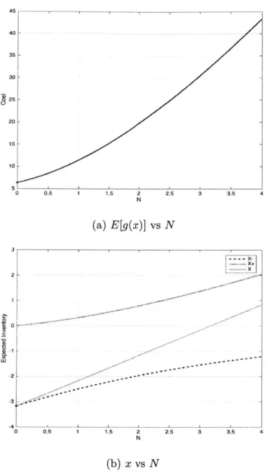
Figure 4-1: Optimal buffer size given equal surplus and backlog costs and unreliable demand, Pi = O.8 95, P2 = .890,g_ = 2, g+ = 2, r1/r2 = O.9, p1/p2 = 0.01

Figure 4-1 shows the optimal buffer size, N*, given equal surplus and backlog costs and unreliable demand. As N increases, the expected backlog to be incurred decreases, but the expected surplus increases at a higher rate. The vice versa is true for the case of N decreasing. The N* in this case is 1.74 with expected cost g = 5.488

and t = -1.41.

Figure 4-2 shows N* if cost of surplus increased to g+ = 20. The optimal N* will be reduced to zero, such that P(x > 0) = 0. This is expected since N* is decreasing

so frequency and magnitude of surplus is reduced in order to minimize cost. N* will decrease to a lower bound of 0, because if N* is negative, you will always be incurring backlog cost. t in this case decreases -3.16 and g = 6.33.

45 -- - - - ---- - -...--- ---- --- ---..-r -- ... 40 35-30 25- 20-10 5 0 0.5 1 1.5 2 2.5 3 35 4 N (a) E[g(x)] vs N 31 *x.i 0~~~- -- - - -- -]--1r. 0 0.5 1 1.5 2 2.5 3 3.5 4 N (b) x vs N

Figure 4-2: Optimal buffer size when surplus cost is increased to g+ = 20, p, =

0.895, P2 = 0.890, g_ = 2, g+ = 20, r, /r 9_{,P/P2 =} 0.01

65 60 55 50 45 40 35 30 25 20 15 0 2 4 6 8 10 12 14 N (a) E[g(x)] vs N 10 4 -0 -2 0 2 4 6 8 10 12 14 N (b) x vs N

Figure 4-3: Optimal buffer size when surplus cost is increased to g = - 20,p, =

0.8 9 5_{, P2 = 0.890, g- = 20, g+ = 2, ri/r}

2 = 0.9,pl/p2 = 0.01

Figure 4-3 shows N* if cost of backlog increased to g_ = 20. N* will now increase to 8.8 in order to reduce P(x < 0) to close to 0. t in this case is 5.68 and g = 19.69.

4.2.2

Reliable Demand

In this section, we will compared the optimization of the bottomless-buffer, continuous-time, two-machine line with the single-Machine, single-spart-type, time-dependent failure example given in section 9.3 of

[1].

M2 goes down, the system actually requires a larger buffer, because when M2 gets

repaired, it will consume inventory at a higher A2 and the expected backlog to be

incurred becomes higher.

Figure 4-5 shows that if the cost of surplus is significantly increased, the optimal policy is to make the buffer size N equal to 0. Just like the unreliable case, the system will no longer hold any inventory in order to avoid the surplus cost. Here, optimal cost is 3.8 and * = -1.89. Notice that the optimal cost is exactly g_2*, since the system will never incur surplus.

Figure 4-6 shows that if the cost of backlog is significantly increased, the optimal policy is to make the buffer size N larger, N*=5.75, optimal cost is 13.47, just like the unreliable case. Here, z = 3.83.

S --- -- - ---- --- --- --- ---...---...--....----... ..---..--- -* - - r --- - "--- ---- ---- *T---*1 - ---- op-depend-nI - - i e-- ndent 75 .. 5,5 5-5.5 4.5 4 35 0 0.5 1 1.5 2 2.5 3 3.5 4 4.5 5 N (a) E[g(x)] vs N 4 -3. 2 Ix if --2 --- - -- -- - --- .---- -- --- --- - - -0 5 1 15 2 25 3 3.5 4 4.5 5 N (b) x vs N

Figure 4-4: Optimal buffer size given reliable demand with equal surplus and backlog cost, pi = 0.895, P2 = 0.890, g 2,g = 2, r, = 0.9, Pi = 0.01, p2 = 0

so .-.-..-...-, ---...- ..-- -..- r- - ...-.- --- --- --- --- ---- -- * -... .. ....- op-depend.nt - -time-dependent 50 - 40-30 20 - 10-0 0 0.5 1 1!5 2 2.5 3 3.5 4 N (a) E[g(x)] vs N 3 2.5 15- -~ 0 --1.5 --- ----f . ... ... ..... .. ... ... .... ...I. ... ... ---L... .. ... .1 ... .... L... S 0.5 1 1.5 2 2.5 3 3.5 4 N (b) x vs N

Figure 4-5: Optimal buffer size given reliable demand with surplus cost increased to

0 1 2 3 4 5 6 7 8 9 N (a) E[g(x)] vs N 20 is 10 10 8 (b) x vs N

Figure 4-6: Optimal buffer size given reliable demand with g_ = -20, p1 = 0.895, P2 = 0.890, g- = 20, g+ = 2, r1 = 0.9

backlog cost increased to

,Pi = 0.01,P2 = 0 47 35 30 N25 - -0 -V. --- --- -- ---2 3 46 7 N 6 4 2 0 -2 0 0 ~~

4.2.3

Key Relationships

g+/g-(a) Reliable Demand

ptimal 6upr 8 . Optimaj Cost 12 4 0 02 0.4 0.6 0.8 1 1.2 1.4 1. 1.8 2 gO+g-(b) Unreliable Demand

Figure 4-7: Relationship among the surplus cost, backlog cost, optimal cost, optimal Buffer Size and t, L vs N* I*, E*[g(x)], pi = 0.8 9 5, P2 = 0.890 for both graphs

9-Figure 4-7 shows the relationships among the surplus cost, backlog cost, optimal cost, optimal buffer size and t. As surplus cost increases relative to backlog cost, the buffer size and t decreases, while the optimal cost increases. This is because while the system is decreasing the buffer size to minimize surplus cost, by lowering N*, the frequency and magnitude of backlog is increasing. Thus, the system is now incurring more backlog cost. As expected, the optimal cost 2 and buffer size are higher for the unreliable case relative to the reliable case. The system will hold more inventory to mitigate the uncertainty in demand.

Figure 4-8 shows the behavior of N*, 2* and E*[g(x)] as the ratio of P increases

P2

at a given a 0.02. As the ratio increases, the isolated production rate of M is

in-

9-creasing relative to the demand rate, P2. The optimal buffer size, N*, decreases since less storage space is needed when M, becomes increasingly capable of meeting de-mand. As a result, the expected inventory, *, decreases accordingly and approaches

0 as storage is no longer necessary when isolated production rate of M1 is

signifi-cantly higher than the demand rate. The optimal cost will decrease as storage space and is decreasing, and approach gE[x~]. This is due to the fact that, although as

N* approaches zero, E[x-] will not be zero since the M1 will experience downtimes

such that backlog will occur.

In the unreliable case, N* and T are both higher than that of the reliable case. Since backlog is significantly more expensive that surplus, the system allows for a larger buffer to not only avoid backlog, but also account for the stochasticity. As a result, the cost is also higher. In both cases, the buffer remains quite full, as the difference between N* and T remained small and consistent at 0.110.

Figure 4-9 shows the cases when g+ is increased by a factor of 10. As expected, due to the increase in surplus cost, the system will quickly reduce N* in order to avoid the higher surplus cost. In the reliable case, t becomes slightly negative as pi

is close to P2. This is due to the fact that when N* is 0, t will be negative because when ever M1 is blocked, N can only decrease. As p, improves, M is more capable

at replenishing inventory, thus J becomes close to zero, albeit still negative. In the unreliable case,

zt

--- Xbar

Optimal Buffer Size Optimal Cost

A

11 1 1.2 1.3 1.4 1.5 1.6 1.7 1.8 1,9 2

rho 1/rho2

(a) Reliable Demand

6 -- Optimal Buffer SizeJ

14 ... Optimal Cost .t11,6 *1-4 110 4 -0.6 .02 --- L . ... __ _ ...__ ......_ ..._..._... __ __ ... ...__ .__ ..._ 1 1.2 1.3 1.4 1.5 1.6 1.7 1.8 1.9 2 rhol /rho2 (b) Unreliable Demand

Figure 4-8: Behavior of N*, V* and E*[g(x)] as the ratio of P' increases at a given

S =0.02, P- vs N*, V*, E*[g(x)]. =0.02

-. .Xbar .. <.Optimal Bufer Size

. Optimal Cost 1. -* it it O.S - - - -1 1.1 1.2 1.3 1.4 1.5 1.8 1.7 1.8 1.9 2 rhol /rho2

(a) Reliable Demand

S . -Xar 1 1.5 rhol/rho2 1.6 1.7 1.8 1.0 -~6 -4 A 2 (b) Unreliable Demand

Figure 4-9: g+ is increased by a factor of 10, P vs N*, x*, E*[g(x)]. =0.2

7

Ii

4

3

~ ---- Optimal Buffet Size

... Optimal Cost-. -.... ...

C,

.2 ...... "

1 1.1 1.2 1.3 1.4"""3""T23--senaeumenommuunces.ms"emessmanm) e I

Chapter 5

Conclusion and Future Research

We have presented a model and methodology to analyze a two-machine continuous flow system with a buffer of finite capacity, but with unlimited backlog (bottom-less). Each machine is modeled with a single up and a single down state, subject to operationally dependent failures. In this two machine model, the first machine can be interpreted as supply, while the second can be interpreted as demand. We then considered the problem of selecting an optimal buffer size, N*, that minimizes total inventory cost of the system. The optimization methodology allowed us to un-derstand the complex tradeoff between expected surplus and expected backlog given varying levels of costs and production rates. It was also shown that this model given reliable demand closely resembles the time-dependent failure model of the hedging point policy described by

[1].

Equations (2.14) thru (2.16) in state-space form. A analytical solution to A, and A2 can be obtained. Further work needs to be carried out to show at least

one such A is non-positive.

2. A long-line continuous flow model with a bottomless buffer in end of the line. This is a more robust model representing factory production line and stochastic demand for its final finished goods inventory. Optimization can then be added to optimize inventory buffer levels throughout the production line and the hedging point policy that minimizes inventory costs.

Appendix A

Derivations

f=

S S

]xek'dx

+

Derivation of Equation (4.5) E+[x] = E[xlx > 0]P(x > 0) 2 2 2 N j=1 al=l a2=1 xf(xlx > 0)P(x > 0)dx + NP(N,a1, a2|x I 0)P(x > 0) + NP(N, a1, a2)

IN

7I

ZZZ

J

7

Bibliography

[1] Stanley B. Gershwin. Manufacturing Systems Engineering. Fourth Private

Print-ing, Cambridge, Massachusetts, 2011.

[2] Gershwin, S. B. & Schick, I. C. (1979) Analytic Methods for Calculating

Per-formance Measures of Production Lines with Buffer Storages. Proceedings of the 1978 IEEE Conference on Decision and Control. San Diego, California, 618-624.

[3] Stanley B. Gershwin & Oded Berman (2007) Analysis of Transfer Lines Con-sisting of Two Unreliable Machines with Random Processing Times and Finite Storage Buffers. A I I E Transactions, 13:1, 2-11,

[4] Baris Tan & Stanley B. Gershwin (2009) Analysis of a general Markovian two-stage continuous-flow production system with a finite buffer. International Journal

of Production Economics, 12:2, 327-339.

[5] Dallery, Y., David, R., & Xie, X. (1988) An efficient algorithm for the analysis of transfer lines with unreliable machines and finite buffers.. IE Transactions, 20:3, 280-283.

[6] Gershwin S. B. (1987) An efficient decomposition algorithm for the approximate evaluation of tandem queues with finite storage space and blocking. Operations

Research, 35, 291-305.

[7] Burman M. H. (1995) New results in flow line analysis. Ph.D. thesis,

Mas-sachusetts Institute of Technology. Cambridge, MA.. MIT Laboratory for

Manu-facturing and Productivity, Cambridge, MA..

[8] Colledani, M & Gershwin, S. B. (2013) A decomposition method for approximate evaluation of continuous flow multi-stage lines with general Markovian machines.

Annals of Operations Research, 209:1, 5-40.

[9] Bielecki, T & Kumar, P. R. (1987) Optimal Inventory Levels for an Unreliable Manufacturing System: Necessary and Sufficient Conditions for a Zero-Inventory Policy to be Optimal. IFAC Proceedings, 10:5, 159-160.