Axisymmetric theory and the interactive, asymmetric monsoon

(1)

Axisymmetric Theory and the Interactive, Asymmetric

Monsoon

by

Nikki C. Priv6

B.S. Mechanical Engineering

University of Maryland, College Park (1999)

M.S. Atmospheric Science

Massachusetts Institute of Technology (2002)

Submitted to the Department of Earth, Atmospheric, and Planetary Science in partial fulfillment of the requirements for the degree of

Doctor of Science in Atmospheric Science at the

MASSACHUSETTS INSTITUTE OF TECHNOLOGY

June 2005

@

Author...

...

... ...

Department of Earth, Atmosph ic, and Planetary Science April 28, 2005

Certified by... ...

~- R. Alan Plumb

Director, Program in Atmospheres, Oceans, and Climate Professor of Meteorology Thesis Supervisor

Accepted by ...

E.A. Griswold Professor of

. . . .. . . .. . . .. . . . .. . . ..

Maria Zuber Head of Department Geophysics and Planetary Science

(2)

(3)

Axisymmetric Theory and the Interactive, Asymmetric Monsoon by

Nikki C. Priv6

Submitted to the Department of Earth, Atmospheric, and Planetary Science on April 28, 2005, in partial fulfillment of the

requirements for the degree of Doctor of Science in Atmospheric Science

Abstract

The applicability of axisymmetric theory of angular momentum conserving circulations to the large-scale steady monsoon is studied in a general circulation model with idealized

representations of continental geometry and simple physics. The axisymmetric theory is expanded to explain the the location of the monsoon; assuming quasi-equilibrium, the poleward boundary of the monsoon circulation will be colocated with the maximum in subcloud moist entropy, with the monsoon rains occurring slightly equatorward of this maximum. Starting from an axisymmetric aquaplanet framework, the model complexity is incrementally increased to include first a subtropical continent, then eddies and zonal variation in the flow, and finally asymmetry of the large-scale forcing. It is found that the meridional circulation which develops over a zonally symmetric continent is in good agreement with the axisymmetric theory, but a cross-equatorial meridional circulation does not form over a continent of limited longitudinal width, where the flow is highly asymmetric. The equator proves to be a substantial barrier to boundary layer meridional flow; flow into the summer hemisphere from the winter hemisphere tends to occur in the free troposphere rather than in the boundary layer. The monsoon location is found to be strongly correlated with the maximum subcloud moist entropy, both in the modeled cases and in observed monsoons around the globe. The net effect of eddies is a slight weakening of the monsoon due to redistribution of the moist entropy field. Advection is found to strongly shape the overall distribution of subcloud moist entropy, and to limit the range of the monsoon circulation and precipitation.

Thesis Supervisor: R. Alan Plumb

Title: Director, Program in Atmospheres, Oceans, and Climate Professor of Meteorology

(4)

(5)

Acknowledgments

Where could I possibly begin, save for at the beginning? To my parents, for cake via postal service, for letting me use various power tools, and for not asking too many questions. To six years of housemates, especially Geoff, Josh, and Lenny, for putting up with the fish sauce, and fabric in the shower. To my friends from Blair, for cards at 5 a.m. and a reminder that there is life after school. To my friends from MoW and Grey's, for amusing emails, for encouraging my pyromania, and for Tanc's impressions of Henreitta Pussycat and Stephen Hawking. To Deepika, for helping me with a new hobby, plus all the wonderful people at PR. To Elaine -you still need to cut my hair!

To my advisor, Alan Plumb, for many helpful discussions and for finding my spelling mistakes. To my committee: Elfatih Eltahir, Kerry Emanuel, and John Marshall, for useful suggestions and different viewpoints. To Will Heres, for computer assistance with a sense of humor. To Olivier Pauluis, for holding my hand through the setup of the MITGCM. To Chris Hill, for fixing lots of esoteric computer problems and for scrounging access to better machines. To Ed Hill and Jean-Michel Campin, for debugging my hare-brained programming mistakes. To Prof. Gadgil, for asking a question that lead to a large portion of the final thesis.

Many people have helped to make my stay here more tolerable, even enjoyable at times. To Mary Elliff, for enthusiasm and for understanding the importance of tea. To my year-mates, Rob Korty, Peter Huybers, and Arnico Panday, for Thursday night sessions at the chalkboard. To my lab-mates, Jessica Neu, Alan Kuo, Kirill Semeniuk, Mike Ring, and Ivana Cerovecki, for arguments about the weather and for putting up with open-air headphones. To my officemates, Tieh-Yong Koh, Fabio Dalan, Irene Lee, Yang Zhang, and Roberto Rondanelli, for letting me hog the best corner of the office for my plants and a barely-used desk. To Greg Lawson, Jeff Scott, Bill Boos, Cegeon Chan, and David Flagg, for afternoon and late-night chats. To the bridge-players, who never call the director on me.

To the soft, gentle darkness of the lab at night, and the little things that make life easier. To my car, I promise to buy you a new battery and some tires this year. To the CT2, for four years of speedy, if not timely, service. To the 80, for timely, if not frequent service. To rec.arts.sf.written, for new additions to my library. To Death By Chocolate, so tasty!

This document is quite long, and somewhat tedious to read. Actually, quite tedious, es-pecially chapters 3 and 4. To ease your way through, I have some musical recommendations, as follows: Chapter 1, 76-14, Global Communications; Chapter 2, 6 and 12 String Gui-tar, Leo Kottke; Chapter 3, Stalker, Robert Rich and B. Lustmord; Chapter 4, Courier, Richard Shindell; Chapter 5, garbagemx36, Autechre; Chapter 6, Little Peppermints,

(6)

Antje Duvekot, just put track 5 on repeat.

NCEP reanalysis data provided by the NOAA-CIRES Climate Diagnostics Center, Boul-der, Colorado, USA, from their web site at http://www.cdc.noaa.gov/. ERA-40 reanalysis data provided by the European Centre for Medium-range Weather Forecasting, from their web site at http://www.ecmwf.int/research/era/.

This material is based upon work supported under a National Science Foundation Gradu-ate Research Fellowship. Any opinions, findings, conclusions or recommendations expressed in this publication are those of the author and do not necessarily reflect the views of the National Science Foundation.

(7)

... I must confess, that in this latter occurs a difficulty, not well to be accounted

for, which is, why this Change of the Monsoons should be any more in this [Indian] Ocean, than in the same Latitudes in the Ethiopick, where there is no thing more certain than a S.E. Wind all the Year.

These are particulars that merit to be considered more at Large, and furnish a sufficient Subject for a just Volume; which will be a very commendable Task for such, who being used to Philosophick Contemplation, shall have leasure to

apply their serious thoughts about it.

(8)

(9)

Chapter 1 Introduction

In the summer of 2004, flooding from heavy monsoon rains in southeast Asia resulted in the deaths of more than two thousand people. Millions were displaced from their homes, three quarters of the country of Bangladesh was submerged in flood waters, and billions of dollars of crops were lost (DER Subgroupi, 2004). Rainfall during the monsoon season accounts for a large percentage of the annual precipitation in west Africa, southeast Asia, and northern Australia, and these regions rely heavily on monsoon rains to support agriculture. During the 1970s and 1980s, the west African monsoon was particularly weak over the Sahel region, resulting in widespread drought and famine; the causes of this failure of the monsoon are still not fully understood. Nearly one quarter of the globe can be considered to have a monsoonal climate, although the Asian monsoon is the largest and most prominent of the worldwide monsoons.

Although monsoons strongly impact society, agriculture, and economics around the globe, there has been relatively little advance in our understanding of mechanisms which drive monsoons since Halley's 1686 depiction of flow in the tropics. Accurate predictive capabilities for future monsoon seasons do not currently exist, but would be invaluable for saving lives and property and for agricultural planning. Reliable forecasting requires a thorough understanding of the basic dynamics of the monsoon; this will be the focus of this thesis.

1.1 Observed Features of the Worldwide Monsoon

The monsoon is fundamentally a seasonal reversal of wind direction, with the term monsoon derived from the Arabic mausim, or season. During the summer, the monsoon is generally accompanied by heavy rains, with dry conditions during the winter months. Areas close

(12)

100 Asia Australia

100 1 00WN

300

300 -60S

30S

EQ

30N

60N

eS

30S

EQ

30N

60N

to 10

Figure 1-1: Summer zonal mean flow on the latitude-height plane from long term monthly mean NCEP reanalysis data. Vertical velocity in units of 1E2 Pa/s, meridional flow in m/s. Left, mean July flow over Asia averaged between 60E and 120E. Right, mean February flow over Australia averaged between 120E and 160E.

to the equator are not monsoonal because there is no seasonal reversal in wind direction, although they may experience intense precipitation from the intertropical convergence zone (ITCZ). Monsoon regions are located in the tropics and subtropics, far enough from the equator that seasonality exists, but where tropical convection remains a strong player in local climate. Observed monsoons exist over Australia, southeast Asia and India, Amazonia, West Africa, and the North American southwest.

Continents feel seasons more strongly than oceans due to the much smaller heat capacity of soil in comparison to water. During summer, land surfaces tend to heat quickly, strongly forcing the atmosphere above, while the ocean stores much of the incoming radiative energy internally and shows a slower and weaker seasonal response. Since the monsoon is a response to seasonal forcing, it is closely associated with continental areas; however, it has been proposed that a localized, positive, subtropical SST anomaly could also result in a monsoon (Yano and McBride, 1998), were there some mechanism for producing such an anomaly.

The zonal mean flow in the monsoon area shows strong, deep ascent over the monsoon region as part of a cross-equatorial circulation with subsidence in the opposite hemisphere (Figure 1-1). This circulation has the character of a broad Hadley circulation, and has been interpreted as the relocation of the ITCZ into the monsoon area (eg. Gadgil (2003)). The zonal wind field features upper level easterlies over the tropics, flanked by a strong upper level westerly jet in the winter hemisphere subtropics and a weaker upper level westerly jet in the summer hemisphere midlatitudes (Figure 1-2). The easterlies extend down to the

(13)

Figure 1-2: Summer zonal mean zonal wind on the latitude-height plane from long term monthly mean NCEP reanalysis data, units m/s. Left, mean July flow over Asia averaged between 60E and 120E. Right, mean July flow over west Africa averaged between 1OW and 10E.

surface in the winter hemisphere tropics, with weak easterlies or near zero winds at the surface on the poleward edge of the monsoon. Westerly winds exist at low levels between the equator and the monsoon where air is carried poleward, retaining relatively high angular momentum from the equator.

The horizontal flow associated with the monsoon is complex. A large cyclonic circulation develops over the monsoon region in the lower troposphere in response to the heated land surface. Equatorward of this cyclone, significant cross-equatorial flow carries moisture from the tropical ocean into the monsoon area (Figure 1-3). Aloft, a divergent anticyclone develops with outflow from the monsoonal ascent. The anticyclone associated with the Asian monsoon is particularly large, spanning much of Asia and northern Africa, as shown in Figure 1-4. Precipitation associated with the monsoon can be very intense and occurs over a large area, primarily along the coastline. As the summer progresses, the rain spreads further inland; in Asia and Australia, the precipitation maximum remains near the coast, whereas the precipitation maximum in the African monsoon moves inland while the coastal precipitation wanes.

The monsoon has strong intraseasonal variability over a range of time scales. On time scales of a few days exist monsoon depressions, synoptic scale low pressure systems which are responsible for the majority of monsoon precipitation. On a monthly timescale, the monsoon experiences an active/break cycle which strongly impacts agricultural interests. During the active phase, the strongest precipitation occurs over the landmass, while during

(14)

20 m/s 40 5 35 4.5 30 4 25 3.5 20 3 15 2.5 10 2 5 1.5 -10 0 40 50 60 70 80 90 100 110 120 130 140 Longitude

Figure 1-3: Long term mean July flow in the Asian monsoon region, from ECMWF

reanal-ysis data. Contours are precipitation, contour interval 0.5 mm/day; vectors are boundary

layer horizontal winds.

the break period the rainfall maximum shifts equatorward and occurs over the ocean just off of the coast; each phase may last several weeks. The causes of this variation between active and break regimes are not well understood, and are beyond current forecasting capa-bilities. On the seasonal timescale, the Asian monsoon experiences delayed onset: the wind reversal and initiation of continental precipitation occur approximately one month after the landmass reaches high surface temperatures (Xie and Saiki, 1999). This phenomenon is poorly modeled in most general circulation models, and is again not well understood.

1.2 Axisymmetric Theory

Angular momentum has long been known to have a strong impact on the steady zonal mean circulation in the atmosphere. An early depiction of meridional circulation in the tropics was made by Hadley (1735), who reasoned that differential heating by the sun leads to a direct overturning cell with ascent in the tropics where heating is strongest, and with

(15)

Figure 1-4: Long term mean July streamlines at 150 mb in the Asian monsoon region, from

NCEP reanalysis data.

subsidence at higher latitudes. Hadley hypothesized that conservation of absolute angular momentum of the low-level equatorward flow would yield the observed easterly flow in the tropics.

Conservation of angular momentum acts to constrain the steady state zonal wind field. Hide (1969) noted that superrotation at the equator in the absence of sinking motions requires local longitudinal pressure gradients, as this is the only force which can increase the angular momentum of the atmosphere to a value greater than that of the solid earth at the equator. This was generalized by Schneider (1977) to show that in a viscous, axisymmetric framework, extrema of absolute angular momentum must occur in a region of a source or sink of momentum, so that such extrema are confined to the lower boundary of the atmosphere in the absence of sources or sinks aloft. The net advective flux of momentum across a contour of constant angular momentum must be zero: advection cannot compensate for a diffusive friction which has a downgradient flux of momentum across contours of constant momentum. Any extremum of angular momentum which exists away from the bottom surface would be destroyed by viscous processes and cannot be maintained in a steady

(16)

state.

Schneider noted that under axisymmetry, the tropical temperature field is controlled by the requirement there exist no extrema of angular momentum, so that meridional gradients of temperature must be small. The assumption of a particular temperature field with no meridional flow and with zonal wind in thermal wind balance with temperatures may be invalid if an extremum of angular momentum would result. Instead, a meridional circulation of sufficient strength to homogenize temperatures in the tropics is needed.

Held and Hou (1980) used the concepts developed by Schneider (1977) to focus on the annual-mean meridional circulation by assuming a radiative-convective equilibrium (RCE) state with maximum temperatures at the equator. A wind field with flow in thermal wind balance with the radiative convective equilibrium temperatures cannot develop for this case, as upper level westerlies would result at the equator, which are not allowed. Instead, an angular-momentum conserving (AMC) meridional circulation develops with two cells, each with ascent near the equator and subsidence in the subtropics, with equatorward flow in the boundary layer and poleward flow aloft. The flow carries high angular momentum air from the equatorial region into the subtropics in the upper troposphere, where westerly jets form along the boundaries of the circulation cells. Poleward of these boundaries, the thermal equilibrium solution is in balance with the RCE temperatures.

Lindzen and Hou (1988) extended this theory to the case where there is a nonzero gra-dient in RCE temperature at the equator - in thermal equilibrium, this would result in infinite zonal wind speeds near the equator and a discontinuity with westerlies on one side and easterlies on the other. As this thermal wind distribution is not allowed on several counts, an AMC meridional circulation develops instead. Two circulation cells form, one large 'winter' cell featuring ascent poleward of the latitude of the RCE temperature max-imum and cross-equatorial flow with subsidence in the winter hemisphere, and a second, much weaker circulation cell in the summer hemisphere, poleward of the ascent region. The zonal wind field again features strong westerly jets at the subtropical edge of the circulation, but in this case there is an equatorial easterly jet resulting from conservation of angular momentum as off-equatorial air is transported to the equator. As the RCE temperature maximum is shifted poleward off of the equator, the cross-equatorial circulation broadens and strengthens considerably; this cell is considerably stronger than the symmetric cells found by Held and Hou (1980). Observations show that the real atmosphere features a circulation similar to that descibed by Lindzen and Hou (1988), with a dominant winter cell, during most of the year; the annual-mean circulation with two cells of equal size and with equatorial ascent occurs only briefly after equinox.

Plumb and Hou (1992) examined the circulation induced by a localized subtropical forcing with zero gradient in RCE temperature across the equator. For weak forcing, the

(17)

U

EQ

Figure 1-5: Diagram of zonal winds (blue) and meridional circulation (red) for subthreshold forcing.

thermal equilibrium solution is permissible, with RCE temperature distribution throughout the globe. In this regime, the meridional flow is weak and viscously driven, and the zonal wind is in thermal wind balance with the temperature (Figure 1-5). For strong forcing, zonal wind in the thermal equilibrium solution would result in an extremum of angular momentum in the upper troposphere; instead, a meridional circulation develops which redistributes the temperatures in the tropics. This strong circulation cell is cross-equatorial in extent, and conserves angular momentum, forming an upper level easterly jet near the equator (Figure 1-6). The critical condition for the development of a meridional circulation is the existence of an extremum of angular momentum in the thermal equilibrium solution, which can be rewritten as the vanishing of absolute vorticity in the thermal equilibrium solutions. The forcing strength needed to reach this threshold is dependent on the latitudinal distribution of the equilibrium temperatures through

1 gD 1 _0 cos3#oTe

1

<2Q2_a2_siosCq5

( 2 To cos# 0# 1sin# 0#

where g is the acceleration of gravity,

#

is the latitude, D is the height of the tropopause,

To is a reference temperature, Te is the depth-averaged radiative-convective equilibrium

temperature, and a is the radius of the earth. Plumb and Hou hypothesized that the abrupt onset of the monsoon might be related to this threshold behavior, with the thermal equilibrium solution during the pre-onset period switching to the AMC regime as the surface forcing reaches the threshold strength.

(18)

u

EQ

Figure 1-6: Diagram of zonal winds and meridional circulation for supercritical forcing as in Figure 1-5.

Emanuel (1995) showed that the threshold conditions can be written in terms of the subcloud moist static entropy for a moist convecting atmosphere. Assuming a moist adi-abatic lapse rate, and making use of the Maxwell relations, the threshold may be written as

(TS - Tt) -4 2a2_cos3

#sing (1.2)

(9# sin#

8#

where 8

b is the subcloud moist entropy, T, is the surface temperature, and Tt is the tem-perature at the tropopause. Zheng (1998) verified the behavior in a moist axisymmetric aquaplanet model.

Schneider (1983) also examined the atmospheric response to a localized (6-function) forcing, and found that two different regimes of AMC circulation are possible, depending on the strength and location of the forcing: a 'local' circulation which is confined to one hemisphere, and a 'global' circulation which is nearly symmetric about the equator. There are two thresholds for the behavior of the circulation. For weak forcing below the first threshold, only the local circulation is possible, although this circulation is AMC unlike the local viscously driven circulations found by Plumb and Hou. Both local and global circulations are possible for forcing above the first threshold and below the second; above the second threshold, only the global circulation can attain. The magnitude of forcing at the two thresholds is dependent upon the location of the forcing region; the forcing magnitude increases as the forcing is shifted poleward.

(19)

Tung (1996) and Fang and Tung (1997). Deep moist convection acts to rapidly communicate subcloud conditions throughout the depth of the troposphere so that the vertical profile of temperature and humidity approaches a moist adiabat. The effects of moist convection can be represented as very short Newtonian cooling timescale in local areas of deep convection, with a longer 'dry' timescale elsewhere. The strength of the circulation is dependent upon the longer cooling timescale in subsiding regions, while the temperature in the tropics is determined by the local temperature in the area of ascent and deep convection. In a moist atmosphere, the ascent branch of the circulation narrows and the vertical velocity increases in comparison to a dry circulation.

1.3 Simple models of the monsoon

The first published depiction and explanation of the monsoon was written by Halley (1686), who put forth the hypothesis of the monsoon as a giant sea-breeze circulation. In the winter, the land is cooler than the nearby ocean, causing equatorward flow from the continent toward the ocean; while in the summer the land is warmer than the ocean, inducing the opposite flow pattern with rising air over the land leading to precipitation. This simple theory remained uncontested for several hundred years, and the sea-breeze paradigm is still seen in textbooks and popular science articles today. However, the sea-breeze theory fails to account for the abrupt onset of the Asian monsoon and the active/break cycle. The sea-breeze paradigm also neglects the rotational effects which are significant at the large horizontal scales of the monsoon.

Gill (1980) explored the response of a linear shallow water model on the

#-plane

to localized forcings centered both on and off of the equator. When the forcing is centered north of the equator, a region of ascent is colocated with the applied forcing, and pressure minimum is offset to the northwest of the forcing (Figure 1-7). To the east of the forcing, a tropical Kelvin wave signature is seen, with easterly flow but no meridional flow. A Rossby-wave regime exists to the west of the forcing, strongly biased to the northwest of the forcing, with cyclonic flow around the low-pressure region and westerlies near the latitude of the forcing. There is also a significant signal in the southern hemisphere, with cross-equatorial flow to the south and west of the forcing. This flow pattern is quite similar to the lower tropospheric flow in the vicinity of the Asian monsoon during summer.

1.4 Cross-equatorial flow

The equator, where the Coriolis parameter

f

changes sign, is a strong dynamical barrier in the atmospheric mixed layer. In the free troposphere, the atmosphere may be considered

(20)

( ) 0

--4

Figure 1-7: Flow induced in a linear model with localized off-equatorial heat source (from Gill (1980), Figure 3). Top, contours of vertical velocity, arrows show low-level horizontal flow. Bottom, contours show perturbation pressure.

to be almost angular momentum conserving, so that the flow follows contours of angular momentum. The flow may act to homogenize angular momentum in the free troposphere, allowing cross-equatorial flow. However, in the mixed layer, viscous effects are strong and can discourage cross-equatorial flow: the meridional momentum budget is a balance be-tween viscous effects, flow induced by mixed-layer temperature gradients, and flow induced by geopotential gradients just aloft of the mixed layer. Because of angular momentum conservation in the free troposphere, the mixed-layer meridional flow induced by the free tropospheric geopotential gradient has a latitude-dependent upper bound, which approaches zero at the equator. Therefore, a temperature gradient in the mixed layer is needed in order to induce a cross-equatorial flow.

Pauluis (2001) has addressed the difficulties in achieving low-level cross-equatorial flow in an axisymmetric framework. For a given mixed layer depth and pressure gradient, there is a maximum possible mass flux that can cross the equator in the mixed layer; this mass flux decreases with shrinking mixed layer depth and with weakening pressure gradient. Thus, if the pressure gradient across the equator is weak, or if the mixed layer is too shallow, the low-level return flow of the Hadley circulation may not be able to cross the equator entirely

(21)

in the mixed layer, and some portion of the flow must rise and cross the equator in the free troposphere. The resulting Hadley cell is horseshoe-shaped, with a 'jump' in the lower branch of the flow at the equator. While the jumping behavior is only weak in dry models, the presence of moist convection and associated precipitation weakens the moist stability of the flow near the equator, and the jumping behavior reaches deep into the troposphere.

The dynamical barrier to cross-equatorial flow may also be described in terms of poten-tial vorticity. A parcel of air which crosses the equator will have potenpoten-tial vorticity which is opposite in sign to the background potential vorticity; the potential vorticity of the parcel must be modified for the parcel to make its equatorial crossing permanent. Rodwell and Hoskins (1995) investigated the effects of surface drag and diabatic heating over the Indian Ocean on low-level cross-equatorial flow. These processes act to modify the potential vor-ticity of the flow, changing the sign of the PV from negative to positive as the flow crosses the equator. If the diabatic processes are not able to change the sign of PV of the flow, the air recirculates into the originating hemisphere in the eastern Indian Ocean.

Investigations into the dynamical mechanisms which allow low-level cross-equatorial flow frequently focus on the response of the tropical atmosphere to a localized, off-equatorial heating. As previously discussed, Gill (1980) achieved significant cross-equatorial flow in a linear, viscous shallow-water model with off-equatorial forcing. Sashegyi and Geisler (1987) examined the response of a linear model of a stratified fluid on a rotating sphere to a prescribed idealized off-equatorial heating. They found a response similar to that of Gill (1980), with two major circulation cells: a zonally-oriented cell with ascent near the heating region and descent to the west, and a meridional overturning cell with cross-equatorial flow and descent in the opposite hemisphere.

Low-level cross-equatorial flow is associated with monsoons across the globe, although the influence of this flow is not well understood. Near West Africa, the flow crosses the equator over the ocean and turns southwesterly as it approaches the coastline during the monsoon season. Over the western Pacific and Indian oceans, the flow is much more complex (Figure 1-3). Numerous studies (eg. Anderson (1976), Rodwell and Hoskins (1995)) have shown that the presence of Africa and the East African mountain range straddling the equa-tor help to form the Findlater jet. In boreal winter, cross-equaequa-torial flow to the Australian monsoon is impacted by the Maritime continent with its volcanic islands. Cross-equatorial flow also occurs over central South America during boreal winter, with northeasterly flow near the equator turning northerly near 10S and then northwesterly over southern Brazil, perhaps deflected by the Andes mountains. Qian et al. (2002) have shown that the pres-ence of cross-equatorial flow, along with seasonal variation in precipitation, can be used to identify monsoonal regions around the globe. One exception is the North American sum-mer monsoon, for which there is no clear area of associated cross-equatorial flow; instead,

(22)

southeasterly flow over the warm Caribbean Sea and western Atlantic ocean converges over the North American monsoon region.

The presence of the East African jet, first discovered by Findlater (1969), has focused attention on the role of orography in inducing cross-equatorial flow. During boreal summer, cross-equatorial flow is found in the western Pacific and in a narrow jet along the western Indian Ocean, but there is little cross-equatorial flow in the central and eastern Indian Ocean. Easterly winds crossing the Indian Ocean encounter the East African Highlands, forcing the wind into an intense but narrow low-level cross-equatorial jet along the eastern coast of Africa. This jet accounts for a significant percent of the global total cross-equatorial flow, and is thought to strongly impact the monsoon in the Indian subcontinent. Hoskins and Rodwell (1995) found that the removal of the East African orography in their model lead to a large decrease in the strength of the East African jet. Sashegyi and Geisler (1987) have shown that orography can concentrate the cross-equatorial flow induced by a tropical heat source into a western boundary current, but the net cross-equatorial mass flux is not substantially increased by inclusion of topography.

Moisture budgets taken over the Indian peninsula have shown that cross-equatorial flow supplies a substantial fraction of the moisture needed for monsoon precipitation (Ninomiya and Kobayashi (1999), Kishtawal et al. (1994)), although evaporation from the Arabian Sea is also a significant source of moisture for the monsoon. Findlater (1969) found a positive correlation between the strength of the jet and the intensity of rainfall over western India during the monsoon, with the rainfall peaking about 2 days after the peak in jet strength. Cross-equatorial flows are also associated with the southeast Asian monsoon, where local cross-equatorial flow converges over China with flow crossing from the Bay of Bengal (Ninomiya and Kobayashi, 1999).

1.5 Location of the monsoon

The Asian monsoon shows a strong east-west tilt, with the monsoon extending furthest poleward along the east coast of Asia. To the west of the monsoon region, the Saharan desert exists at roughly the same latitude as the Asian monsoon. The Australian monsoon also shows an east-west tilt, but the West African monsoon does not show such a tilt and sometimes has strongest precipitation at the western coast. Numerical studies have suggested various dynamical mechanisms which contribute to asymmetry of the monsoon.

Rodwell and Hoskins (1996) hypothesized that Rossby waves induced to the west of the monsoon (as in Gill (1980)) are associated with subsidence, which in turn discourages moist convection. Using a simple model with prescribed, idealized forcing, they found a broad area of subsidence to the northwest of a subtropical heat source. This effect was examined in

(23)

a model of intermediate complexity with interactive forcing by Chou et al. (2001) and Chou and Neelin (2003). By comparing two cases, one with full spherical geometry, and the other on an f-plane, Chou et al. (2001) found that the Rodwell-Hoskins effect does substantially contribute to the east-west asymmetry of the monsoon. Chou and Neelin (2003) conducted a similar experiment using more realistic continental geometries, and found that the Rodwell-Hoskins effect significantly affected the asymmetry of the monsoon in North America and Asia, but not in Africa.

The strong influence of the large-scale circulation on the geometry of the monsoon has been demonstrated in several studies. Xie and Saiki (1999) found that the low-level cyclonic circulation over the summer continent carries dry continental air into the subtropics along the western edge of the landmass, while moist oceanic air is carried inland along the eastern edge. This suppresses moist convection to the west, while encouraging rainfall in the east. In their model, the feedback between precipitation and soil moisture accentuated this asymmetry, slowing the inland progression of moist convection over the western continent. In a perpetual summer case, the east-west asymmetry of the monsoon was eliminated when sufficient time was allowed to overcome the resistance to precipitation along the western half of the continent.

Chou et al. (2001) considered the effects of advection of moisture and temperature into the monsoon region, which they termed 'ventilation'. When these advection terms were artificially removed while retaining the moisture convergence associated with divergence, monsoon precipitation spread further poleward over the continent. Chou et al. suggested that the advection of low moist static energy air from the cool midlatitude oceans acts to suppress moist convection over the western continent and to limit the poleward extent of the monsoon. In a separate experiment, the ocean heat transport from the tropics into the midlatitudes was increased, raising the subcloud moist static energy in the subtropics and midlatitudes; the resulting precipitation over the continent was greatly increased overall with reduced asymmetry.

1.6 Continental geometry

Relatively few studies have been made using simple continental geometries; most GCM studies use realistic representations of continents, while idealized rectangular continents are only favored for less sophisticated numerical models. Two exceptions to this are the work of Cook and Gnanadesikan (1991) and Dirmeyer (1998), both of which used a simplified continental geometry with a full GCM.

Dirmeyer (1998) experimented with the latitudinal positioning of a single rectangular continent, and found three different dynamical regimes of the monsoon. When the coastline

(24)

was located in the tropics, year-round continental precipitation was observed; when the coastline was located in the subtropics, a seasonal monsoon was observed with summer precipitation in the southeast corner of the continent; when the coastline was located in the midlatitudes, a "Mediterranean" climate was seen, with dry summers and wet winters over the landmass. For the subtropical continent cases, the monsoon was primarily supplied with moisture by the tropical easterlies, with little moisture transport across the southern coastline. The longitudinal width of the continent did not strongly affect the monsoon for the subtropical case; the monsoon was weakest when a continent of 3600 width was used, in which case the moisture supply by easterlies from the ocean was lost. However, in the subtropical cases the ITCZ never shifted onto the continent and instead remained in the southern hemisphere year-round; the summer monsoon precipitation was relatively weak.

Cook and Gnanadesikan (1991) used a rectangular continent centered on the equator with simplified hydrology in a perpetual summer experiment. They found that moisture availability over the continent restricted the extent of subtropical precipitation: in a case with a swamp continent, summer subtropical precipitation extended fully across the width of the landmass. But in a case with interactive bucket hydrology, the continent rapidly became arid, and subtropical precipitation was limited to the eastern side of the continent, where easterlies carried moist oceanic air inland. Chou et al. (2001) used a similar continental geometry in an experiment with seasonal cycle, and found that when ocean heat transport was neglected, monsoon precipitation over the interior of the continent was very weak for cases with interactive surface hydrology.

The weakness of monsoon precipitation in many of the modeling experiments with an equatorially centered continent raises a question: is an east-west coastline necessary to produce a robust monsoon? Xie and Saiki (1999) found that onset of the monsoon was caused by baroclinic waves of a low-level easterly jet along the coastline - without the coastline and subsequent meridional temperature contrast, these waves might not exist. The warm tropical ocean along the coastline also acts as an important moisture source for the monsoon; the minimal precipitation seen in the continental interior in experiments with an equatorially-centered continent supports the importance of a nearby moisture source. This has implications for paleoclimate; for instance, the equatorially-centered continent of Pangea existed during the Permian.

1.7 Goals of this Work

There are two different dynamical models of the steady monsoon: the Gill (1980) model of the response to a localized off-equatorial heat source as an additive function of linear Kelvin and Rossby wave regimes; and the axisymmetric, nonlinear model of Plumb and Hou (1992)

(25)

which considers the monsoon as a Hadley circulation with subtropical ITCZ. This study focuses on the nonlinear, axisymmetric theory, to determine how well this framework can describe the dynamics of the three dimensional monsoon.

There is a wide gap in modeling the monsoon between the highly idealized axisymmetric theory and full GCM studies with realistic physics. While the axisymmetric theory is useful for developing an understanding of the basic physical mechanisms which drive and affect the monsoon, it is unclear how the simplifications which are involved limit the applicability to the fully three dimensional monsoon. On the other hand, the wealth of feedbacks present in the full GCM studies make diagnosis of the monsoon behavior extremely difficult. The goal of this work is to bridge the gap between the idealized axisymmetric theory and the

more complex three dimensional monsoon.

The major questions which we wish to address are:

1) How well does axisymmetric theory represent the fully three dimensional monsoon? 2) What determines the strength and location of the monsoon?

A general circulation model with simplified representations of some physical processes and with idealized continental geometry is chosen to achieve intermediate complexity. This allows for a reasonably more realistic portrayal of processes which are suspected to be intrinsic to the monsoon, while at the same time reducing the feedbacks to make analysis more tractable. The complexity of the model geometry is gradually increased from an axisymmetric to an asymmetric framework. By comparing the changes which result from each incremental increase in complexity, the various interacting mechanisms which comprise the monsoon can be separated and examined.

We begin by expanding upon the work of Plumb and Hou (1992) and Emanuel (1995). A major limitation of the axisymmetric theory is the use of a prescribed, non-interactive forcing. While Plumb and Hou (1992) assigned a local subtropical anomaly of thermal equilibrium temperature in a dry model, Emanuel (1995) and Zheng (1998) assumed a saturated surface with constant, prescribed temperature and surface wind speeds. How well does the theory apply when a continent with interactive surface forcing is introduced? The theory hinges on the distribution of RCE temperatures at the tropopause; in order to achieve a temperature maximum over the landmass, the surface forcing must be communicated into the upper troposphere. Deep moist convection is very effective at such communication, but dry convection is not. Given an initially arid landmass with little moist convection, how is threshold behavior affected? Axisymmetric theory predicts that the threshold for a global meridional circulation requires increased forcing as the forcing region is shifted poleward. How, then, does the continental location impact the monsoon?

Axisymmetric studies are limited by the exclusion of zonally asymmetric forcing and of horizontal eddies; they cannot explain asymmetry of the monsoon. The Rodwell-Hoskins

(26)

effect is completely neglected in an axisymmetric framework, as Rossby waves do not exist; similarly, the baroclinic eddies which Xie and Saiki found to initiate the monsoon are not included. The model is expanded to a three-dimensional setup, but the surface conditions and continental geometry are kept zonally symmetric; comparison of these results with the two dimensional case will reveal the role of eddies in formation of the monsoon.

Finally, a continent of limited longitudinal extent is introduced to explore the effects of zonally asymmetric forcing. Chou et al. (2001) and Xie and Saiki (1999) found that advection of relatively cool, dry air by the asymmetric circulation contributes to east-west asymmetry of the monsoon by suppressing convection along the east-western edge of the continent. Why is asymmetry seen in the Asian and Australian monsoons, but not in West Africa?

The model is described in Chapter 2; model results from the two dimensional cases are discussed in Chapter 3. Three dimensional model results are presented in Chapter 4, a discussion of the correspondence of the model results to observations is found in Chapter 5, and conclusions are given in Chapter 6.

(27)

Chapter 2 Model

The model used is the MIT General Circulation Model (MITGCM), release 1.0. The GCM consists of a dynamical core coupled to an atmospheric physics package. This chapter will give an overview of the model dynamics and will describe in greater detail the components of the physics package. Some general characteristics of the behavior of the MITGCM will also be discussed.

2.1 Model Dynamics

The dynamical kernel of the model is described by Marshall et al. (2004). The atmospheric MITGCM has been tested extensively against the Held and Suarez (1994) results, although a different physics package was used than that implemented in this thesis.

The model gridspace used in this thesis is a partial sphere between 64S and 64N, with 40 pressure levels in the vertical at 25 mb intervals. A staggered spherical polar grid is used with 4' latitudinal resolution and 60 longitudinal resolution. There is no orography, and the surface is assigned to the 1012.5 mb pressure level. The top of the atmosphere is located at 0 mb; there is no sponge layer at the upper boundary. Lindzen et al. (1968) found that the imposition of a rigid lid results in spurious reflection of vertically propagating waves, and conjectured that this results would also occur with the lid positioned at p = 0. However, Kirkwood and Derome (1977) found that the wave reflection off of a rigid lid at p = 0 does not result in large errors except for in cases of extremely crude vertical resolution. The vertical resolution used in the MITGCM here is relatively high, and the impact of wave reflection off is not expected to be significant. Physical and thermodynamic calculations are made with a 5 minute timestepping interval. The Eulerian flux form of the momentum equations is used, with the quasi-second order Adams-Bashforth method for advection of both momentum and tracers.

(28)

2.2 Atmospheric Physics

The atmospheric physics package acts on a single column. Radiation and cloud physics are not included; instead, the atmosphere undergoes Newtonian cooling with a cooling timescale

of TNC = 60 days.

QNC = 7ITNC - T) (2.1)

where T is the temperature at a gridpoint, and QNC is the cooling rate. TNC = 200 K for

all gridpoints; this profile for TNC is chosen for its simplicity. There is no representation of stratospheric chemistry, and the stratosphere is cooled toward 200 K by (2.1).

The moist convective scheme of Emanuel (1991) is used, including the modifications of Emanuel and Zivkovi6 Rothman (1999). This scheme employs a buoyancy-sorting approach and was designed with the goal of accurately depicting the convective tendency of moisture. The parameters used as part of this scheme have been optimized against observed data from the Tropical Ocean Global Atmosphere Coupled Ocean-Atmosphere Response Experiment (Emanuel and

Zivkovid

Rothman, 1999). The convection scheme also acts to transport momentum through convective updraughts and downdraughts. The convective momentum tendency of horizontal winds is treated as a vertical eddy-flux of velocity which incorporates entrainment and detrainment of the convective drafts (after Gregory et al. (1997)).

The convection scheme includes dry adiabatic adjustment, which is performed over regions which are unstable to unsaturated ascent. Instability of this nature is most common near the surface where strong heating occurs. The horizontal velocities and moisture are considered to mix rapidly in the unstable layer, and are assigned the mean values within the layer. The temperature is redistributed to stabilize the layer while holding the mean enthalpy constant.

A mixed layer of momentum only (not thermodynamic quantities) is included at the lower boundary of the model. The depth of the momentum mixed layer is assigned to be 200 mb for all locations and times; this relatively deep mixed layer is chosen to allow greater cross-equatorial flow than with a shallow mixed layer. There is also a momentum tendency term due to turbulent surface fluxes, of the form

Fs gpcDss* (2.2)

dp8

where Fs is the momentum tendency, p, is the density of the surface air, CD is the surface drag coefficient, U', is the surface velocity, L is a vertical wind profile coefficient, and dp, is the pressure difference between the surface and the first model layer. v* is a modified surface velocity, defined as

(29)

where w,0 is a minimum surface wind speed, WD is a convective downdraft velocity scale,

and v, and u, are the surface meridional and zonal velocities.

Very simple representations of ocean and land surfaces are implemented. A slab ocean is used, with SST profile fixed in time. The standard atmospheric physics package with this version of the MITGCM does not include representations of land surface, so a set of simple land parameterizations was developed. Over land, a bucket hydrology following Manabe

(1969) is used. Surface evaporation is modified by a factor B

Sf1 B > 0.75Bo _(2.4)

0.75B0 B < 0.75Bo

OB =B P -E

at

where B0 is an assigned bucket depth indicating the amount of moisture that can be stored

per unit surface area, B is the current moisture in the bucket per unit area, E is the evap-oration rate, and P is the precipitation rate. Any excess moisture gained by precipitation is considered to be runoff, so that the maximum value for B is B0, and likewise the bucket

moisture content is constrained to a minimum value of 0 cm. For all runs, the land is assigned a uniform bucket depth of 20 cm.

Because a Newtonian cooling scheme is used, the flux balance at the surface cannot be calculated using radiative fluxes. Instead, the net downward flux into the surface (THF) is prescribed as a function of latitude:

THF(p) = LHF(Ts) + SHF(T) (2.5)

where

#

is the latitude, LHF is the latent heat flux into the atmosphere, SHF is the sensible heat flux into the atmosphere, and T, is the surface temperature. The surface temperature and heat fluxes are interdependent and calculated iteratively. There is no diurnal cycle.

The latent and sensible heat fluxes are calculated from bulk parameterizations:

SH F(T8) = 100pCdcp(v* (T, - Tsa) - v'T') (2.6)

LHF (T,) = 100L, p, CdBe(v* (q,(Ts) - q) - v'q') (2.7)

S

v' =m2 + V2 +U2

where SHF and LHF are the sensible and latent heat fluxes from the surface to the atmosphere, Cd is the surface drag, e is an efficiency factor, v' is the perturbation surface wind speed, p. is the air density at the surface, Lv is the latent heat of vaporization at the surface, q. is the saturated specific humidity at the surface, q is the specific humidity of the

(30)

air just above the surface, e, is the saturation vapor pressure, q' is the turbulent specific humidity perturbation scale, cp, is the heat capacity of moist air at constant pressure, Tsa is the temperature of air at the surface, and T' is the turbulent temperature perturbation scale. For all model runs, the ocean surface drag coefficient were set to be 1.2 x 10-3, and the land surface drag coefficients were set to 3.6 x 10-3.

Using a prescribed net radiative flux has the benefits of allowing direct control over the land surface forcing, and of reducing the number of feedbacks between the forcing and the circulation in comparison to a situation with interactive radiation. Fewer feedbacks permit easier diagnosis of the underlying dynamical mechanisms; this helps to avoid one of the main pitfalls of GCMs wherein the dynamics of the flow can be too complex be readily unraveled and understood. However, the loss of these feedbacks makes the resulting flow less realistic; for example, surface temperatures may become very hot over a desert-like land area as there no increase in the outgoing longwave radiation with increased surface temperatures. Radiative feedbacks due to the presence of clouds and the greenhouse effect are similarly neglected. However, direct control of the land surface forcing allows the behavior of the monsoon to be explored in parameter space by testing a range of different forcing strengths.

A Shapiro filter is used to remove numerical noise, similar to hyperdiffusion. The form of the filter used is given by the function S, where

S l=1- oI 1 I(2.8)

Tshap

L

T4 shap

where Tshap is a damping time scale, At is the timestep, 6i, is the grid spacing in the x-direction, and 6_jj_{is the grid spacing in the y-direction. This filter is applied to the horizontal}

velocity fields, temperature, and specific humidity at the end of each time step. An order of n = 8 is chosen for the Shapiro filter with Tshap = At; this filter is strong enough to remove numerical instabilities while allowing the existence of desirable synoptic scale waves. A quadratic vertical viscosity term is included in the GCM, with the coefficient v constant with height and position.

The radiative convective equilibrium calculations are made by neglecting the pressure forcing terms in the horizontal momentum equations and removing the Shapiro filter - no horizontal flow develops and there is no thermodynamic communication between vertical columns.

All model runs are initialized with zero winds and empty buckets over the land surface. The initial fields of temperature and specific humidity were assigned to a standard vertical profile, shown in Figure 2-1. In most cases, a perpetual summer setup is used with no seasonal variation in SST or in land surface forcing. The model is run until an equilibrium state is reached.

(31)

200- 200-400- 400 -600- 600-800- 800-1000'' 1000 200 400 600 800 0 0.005 0.01 0.015 0.02 T q

Figure 2-1: Initial vertical profiles of temperature (left, K) and specific humidity (right, kg/kg).

2.3 Characterizing the MITGCM

As the atmospheric version of the MITGCM used here has not been extensively described in existing literature, the general characteristics of the model behavior will be discussed.

2.3.1 Comparison with Axisymmetric Theory

As the focus of this thesis is on the axisymmetric theory of Hadley circulations, a com-parison with the analytic theory is helpful in characterizing the model behavior. First, the work of Held and Hou (1980) is reproduced in a dry version of the MITGCM. The moist convection scheme is omitted, a stratosphere is added at a height of 12 km, and the equatorially-centered equilibrium temperature profile from Held and Hou (1980) is applied (their equation (2)). The model is spun up from rest until a steady state circulation is attained. Three different levels of viscous forcing are tested: v = 5, 10, and 20 Pa2

/s.

The MITGCM differs from the Held and Hou model in that the atmosphere is not Boussinesq, there is no rigid lid, and there is a momentum mixed layer.

Figure 2-2 shows an example of the resulting meridional circulation. The circulations which occur with stronger or weaker viscosity are similar in extent and strength, although the lower viscosity cases are prone to inertial instability. This instability manifests as stacked inertial rolls, similar to that found by Held and Hou (1980) in their lowest viscosity case.

(32)

- I II I I I I . ... i

..

.

.1

AL

!

-60 -45 -30 -15 0 Latitude I I ,* '. / 1 ~ \ *1 / *i~*. / / ,.-*,~ ( \ I I. i 1 1 j ~ I 1' ~ N. 15 30 45 60

Figure 2-2: 250 day time mean streamfunction, v = 10Pa2Is, solid lines indicate clockwise flow, dashed lines indicate counter-clockwise flow, contour interval kg/s, dash-dot is zero line.

The analytic theory predicts that the poleward limit of the circulation at the tropopause should occur at 28.6*, coincident with the maximum westerly zonal wind. The maximum zonal wind and boundary of the meridional circulation occurs at 300 in the MITGCM, which is in good agreement with the theory. The strength of the circulation is similar to that found by Held and Hou in the numerical cases with viscosity near v = 5m2/S.

The circulations are close to angular momentum conserving, especially with low viscosity. Figure 2-3 shows the upper tropospheric absolute vorticity for all three cases. Angular momentum is uniform in regions with zero absolute viscosity; the viscosity is near zero from the equator to the poleward edge of the circulation in all cases, with a sudden increase beyond the limit of the meridional cell.

The upper tropospheric zonal wind may be predicted by the analytic theory. The surface drag used in the MITGCM is quadratic, unlike the drag used by Held and Hou (1980); the drag is linearized using a mean value of the surface wind speed in order to calculate the theoretical zonal wind field. The predicted surface winds are stronger than the modeled surface winds by a factor of two. The upper tropospheric winds, shown in Figure 2-4, are quite reasonably close to the predicted winds both in the Hadley region and in the midlatitudes. The modeled temperature field (not shown) is also very close to the predicted temperatures.

For comparison, the model is run with the full dynamics, including moist processes, in

0250

500

(33)

20 x 10

Latitude

Figure 2-3: 250 day time mean absolute vorticity at 200 mb. v = 1OPa2_{/s, dash-dot line; v = 20Pa}2_{/s, dashed line.}

v = 5Pa2/s, dotted line;

an axisymmetric aquaplanet setting with SST maximum at the equator.

SST($) = SST - ATsin($)2 (2.9)

where SSTo = 302K, and AT = 28K. The viscosity is set to v = 1OPa2/s. Two Hadley cells form with ascent at the equator and subsidence in the subtropics, as shown in Figure

2-5; a broad precipitation maximum forms at the equator. The size and form of the Hadley

cells are very similar to that found by Held and Hou (1980) and in the dry results, although the circulation is stronger by a factor of three in the aquaplanet case. However, the forcing in the aquaplanet case is meant to correspond to the observed annual mean SST forcing, rather than to correspond to the forcing used in Held and Hou (1980), so that a difference in circulation strength is not unexpected.

2.3.2 General Model Behavior

A test case is performed in 2D on the latitude-height plane, using an aquaplanet setup with SST uniformly warm at all latitudes,

SST(#) = 302K (2.10)

The model is run for 200 days with an initial zero wind field. The circulation which results is extremely weak in comparison to the observed Hadley circulation, as seen in Figure 2-6. Precipitation (not shown) is nearly uniform at 3.79 mm/day at all latitudes. Clearly, the

. ... . . .... ... ... ... ... .... ... ..... ... ... .... ... ... ... ... ... .... ... .. ... ... . .. .... ... ... ... ... ... .. . . . .- - -.- -. -.-.-.-.-. ... ... .. .... .. . .. . ... .. .. .. ... ... .. . .. .. .. .. I MW ................ ...... .. 10

(34)

-120 100- 80-2 60 - ... 40- 20-0 15 30 45 60 Latitude

Figure 2-4: 250 day time mean zonal wind at 200 mb. Theory, solid line; v = 5Pa2/S7

dotted line; v = 1OPa2/s, dash-dot line; v = 20Pa2/s, dashed line.

model does not self-organize to form a robust meridional circulation or localized deep moist convection.

To explore the model behavior in three dimensions, an aquaplanet case is run with summer-like SST distribution:

SST(#) = 302K - 28sin(# - 8N)2

(2.11)

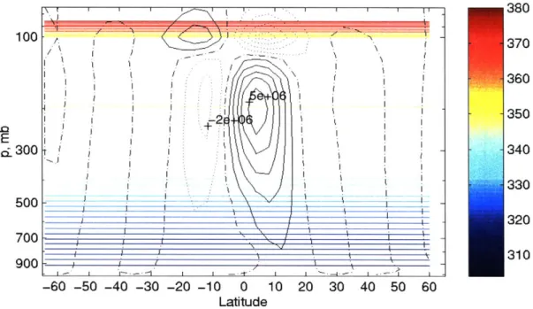
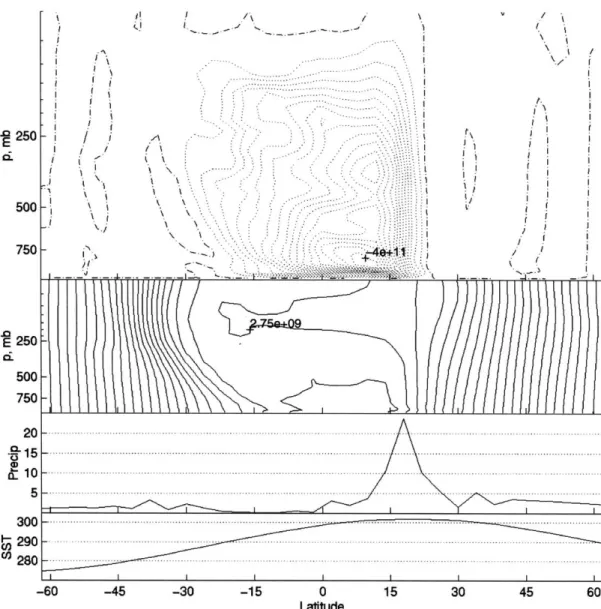
The zonal mean meridional circulation features a cross-equatorial Hadley cell (Figure 2-7) with a smaller local summer Hadley circulation. Eddy-driven Ferrel cells are present in the midlatitudes. The upper tropospheric zonal wind field includes an easterly jet over the tropics flanked by westerly jets on either side. In the lower troposphere, the easterly jets near 10S and 20N result from equatorward flow of the meridional circulation. In the

tropics, there is a broad peak in rainfall, with greatest precipitation near the equator and a secondary maximum in the subtropics near 18N. This subtropical precipitation maximum is related to the strong low level winds associated with the local summer Hadley circulation, which increase surface latent heat fluxes and causes a local maximum in boundary layer moist static energy at 14N.

Approximately 30 days after initializing the model, the westerly subtropical jets develop large eddies. After the initial perturbation of the jets, the dominant wave signals are of wavenumber 5-7 in the subtropics. The Eliassen-Palm flux signature (Figure 2-8) shows baroclinic wave structure in the midlatitudes, with the wave energy becoming barotropic in

Axisymmetric theory and the interactive, asymmetric monsoon