Automation techniques for short interval scheduling in a complex manufacturing environment

Automation Techniques for Short Interval Scheduling in a Complex Manufacturing Environment By

Stephen Paul Baxter

B.S. Mechanical Engineering, United States Military Academy, 2009

Submitted to the MIT Sloan School of Management and the Aeronautics and Astronautics Department in Partial Fulfillment of the Requirements for the Degrees of

Masters of Business Administration And

Master of Science in Aeronautics and Astronautics

_ARCHIVES

In conjunction with the Leaders for Global Operations Programs at ASS C L GY

OF TECHNOLOGY

the Massachusetts Institute of Technology

June 2016 JUN 0 8 2016

2016 Stephen Paul Baxter. All rights reserved.

LIBRARIES

The author hereby grants MIT permission to reproduce and to distribute publicly paper and

electronic copies of this thesis document in whole or in part in any medium now known or

hereafter created. -7 ff Signature of Author: MIT Certified by: Certified by: Accepted by: Accepted by:

Signature redacted

Sloan School of Management, De "frm/f Aert'fautics and Astronautics

Ma A 2016

Signature redacted

Juan Pablo Vielma, Thesis Supervisor Juan Pablo Vielma, Thesis Supervisor Assistant Pressor of Operations Research

Signature redacted

_pervisor

Oli de Weck, Thesis ~prio Professor of Aeronautics and Astronautics and Engineering Systems

___Signature

redacted

__

Paulo Lozano Associate Professor of Aeronautics and Astronautics Chair, Graduate, Program Committee

Signature redacted

__

IfKaura Herso', d5irector ofMT N Program MIT Sloan School of Management

Automation Techniques for Short Interval Scheduling in a Complex Manufacturing Environment

by

Stephen Paul Baxter

Submitted to the MIT Sloan School of Management and the Aeronautics and Astronautics Department on May 6, 2016 in Partial Fulfillment of the Requirements for the Degrees of Master

of Business Administration and Master of Science in Aeronautics and Astronautics. Abstract

Aircraft Company X (ACX) designs and manufactures aircraft. ACX operates Manufacturing Center 1 which produces parts and assemblies for both assembly and spares business lines. Accurate scheduling is crucial for meeting demand and the on time delivery of parts, a key driver of customer satisfaction. Managers currently use a manual process to generate a short interval schedule for production in this volatile, high variety, low volume environment with reentrant flow. The current process is not only time consuming but also disrupts

coordination between supporting functions.

This thesis explores the challenges of developing and implementing an automated scheduling tool in a flexible job shop with re-entrant flow, part families, sequence dependent set-up times, and machine eligibility restrictions. First, a model is developed from current scheduling rules

used by shop floor supervisors. The model uses the earliest due date dispatching rule and part family information to schedule a group of parallel machines. This model is then incorporated into a scheduling tool, which is implemented and tested in the plant. Finally, the results of the implementation are discussed along with improvement to the tool.

The purposed tool demonstrated during testing the ability to save a significant amount of the supervisors' time by reducing their involvement in scheduling, to reduce set-up times by grouping similar parts, and to align support functions by providing a unified build plan for the plant.

Thesis Supervisor: Oli de Weck

Title: Professor of Aeronautics and Astronautics and Engineering Systems Thesis Supervisor: Juan Pablo Vielma

Acknowledgements

First, I would like to thank the MIT Leaders for Global Operations program for its

support of this research. A special thanks goes to my thesis advisors Oli de Weck and Juan Pablo Vielma for their ongoing guidance of this work throughout the internship and thesis writing effort.

Second, I would also like to thank my teammates at ACX for making me feel welcome and a part of the team during my time at the company. Everyone was always willing to help answer my questions and provide insights into operations and scheduling at MCI. I am

especially grateful to Sean whose constant guidance and support was crucial to the success of my internship but also showed me the impact that great leadership can have.

Third, I want to thank my classmates from whom I have learned so much over the past two years.

Finally, I would like to thank my family and friends, whose unwavering support throughout the past two years has made this endeavor possible.

Table of Contents

A b stra ct ... 3

Acknowledgem ents ... 5

List of Figures and Tables ... 9

1 . In tro d u ctio n ... 10

1. 1. Purpose of Project ... 10

1.2. Problem Statem ent ... 10

1.3. Hypothesis ... 10 1.4. Project Goals ... 10 1.5. Project Approach ... 11 1.6. Thesis Outline ... 11 2. Current State ... 12 2 .1. In d u stry ... 12 2 .2 . A C X ... 12 2 .3 . M C I ... 12 2.4. Scheduling ... 13 2.4.1. Reentrant Flow ... 14 2.4.2. Rework ... 14 2.4.3. Due Dates ... .14

2.5. Current Practices and Effects ... 15

3. Literature Review ... 16

3.1. Job Shop Problem (JSP) ... 16

.).2. Parallel M achines and the Flexible Environm ent ... 16

3.3. Flow Shop ... 17

3.4. Implem entation ... 17

4. Approaches to Short Term Schedule Autom ation ... 18

4.1. Fram ework ... 18

4.2. Earliest Due Date ... 19

4.2.1. M otivation ... 19

4.2.2. M ethodology ... 1.9 4.2.3. Initial Results ... 23

4.3. Part Grouping ... 23 4.3.1. M otivation ... 23 4.3.2. M ethodology ... 24 4 .3 .3 . R esu lts ... 2 5 4.4. W ait Tim es ... 26 4.4.1. M otivation ... 26 4.4.2. M ethodology ... 26 4.4.3. Results ... 27 4.5. Initial Conclusions ... 27 5. Implementation ... 28

5.1. Data Stream s and Prediction of Part Flow ... 28

5.2. Dashboard ... 29 5.2.1. Resource Editor ... 29 5.2.2. Taxonom y ... 30 5.2.3. Pacer Charts ... 30 5.3. Adoption ... 30 5.4. Roll-out Plan ... 33 5 .5 . M etrics ... 3 5 5 .6 . R esu lts ... 3 5 U. C onclusion ... 40

6.1. Key Findings and Recom m endations ... 40

6.2. Opportunities for Further Research ... 40

List of Figures and Tables

Figure 1. Current Scheduling Process... 15

Figure 2. Parallel M achine Example... 20

Figure 3. Job A ssignm ent Process... 22

Figure 4. Gantt Chart for Earliest Due Date Exam ple ... 23

Figure 5. Part Grouping ... 24

Figure 6. Set-up Tim e Reduction for Part Grouping ... 25

Figure 7. W ait Tim e... 26

Figure 8. Part Prediction Diagram ... 29

Figure 9. Stake Holder M ap... 31

Figure 10. N ew Scheduling Process ... 34

Figure 11. Supervisor's hours spent scheduling ... 36

Figure 12. Schedule Adherence ... 37

Figure 13. Schedule Adherence Deviations... 38

Figure 14. Actual Set-up Tim e Reduction... 39

1. Introduction

1.1. Purpose of Project

Aircraft Company X (ACX) operates Manufacturing Center 1 (MC 1) that produces parts for multiple demand streams of the business including spares and final assembly. MC1 uses a materials resource planning (MRP) system to schedule the production of parts. The parts are backward scheduled based from due date using the makespan, the total production time for the parts including queue, set-up, and run time for all operations. The MRP system uses a build plan to tell managers what needs to be made; however, it is up to the value stream managers (VSM)

how to assign the various jobs on the individual machines on a daily basis. This manual scheduling process is time consuming. The purpose of the project is to propose methods for automating short term scheduling in MC1.

1.2. Problem Statement

Assess and model current scheduling rules in order to automate short interval scheduling to improve on time delivery to the customer.

1.3. Hypothesis

TIs pr c nypotUhUize aUit iteger prUgaMm11iiig cUn

DC

useu Lo automate the creation of the near optimal short interval schedule for a complex machine shop and the stable scheduling will improve the performance of the shop.

1.4. Project Goals

The goal of this project is:

1) to develop a tool that automates short term scheduling,

2) to evaluate the tool in the current manufacturing environment using performance metrics and

1.5. Project Approach

A phased approach was used to manage the project. The initial phase was current state analysis where interviews and observations were used to gain an understanding of current short term scheduling practices across the plant. During the modeling phase, I built a model to

replicate current scheduling practices. During the prototyping phase, an application, which used the model, was developed and tested.

1.6. Thesis Outline

Chapter 2 provides a background on the industry, ACX, and scheduling at MCI. Chapter 3 is a literary review of academic research into the job shop problem and project implementation. Building on observations made regarding the current state and incorporating the literary review, Chapter 4 outlines three methods for automating scheduling. Chapter 5 discusses the building and implementation of the scheduling tool in MCI. Finally, Chapter 6 summarizes the main points discussed in this thesis and offers concluding remarks.

2. Current State

This chapter provides background of the aircraft industry, ACX, MCI, and scheduling in order to inform the reader on the current state of the problem.

2.1. Industry

The sector of the aircraft industry that ACX competes in expects yearly sales of new aircraft to be around 1200. The sector has five major players that dominate the domestic commercial and military markets. These companies also compete internationally individually and through joint ventures with local partners. Companies generally compete on three different components: price, quality and customer service, and performance. Market estimates put the total demand for civilian turbine aircraft between 4,750 to 5,250 for 2015 to 2019 (Honeywell

Aerospace, 2016). Because military spending is decreasing and oil prices are low, the market for these aircraft is contracting (The Economist, 2015). This downturn has increased competition between the five major players in the aircraft marketplace as consumers continue to expect a very high level of service at a competitive price.

2.2. ACX

Aerospace Company X (ACX) is one of the leading suppliers of military and commercial aircraft and related spare parts and servmcs in the world. The company s subsidiary o" larg

F . , ices i the~ ,~ w. Ic All% % b- L& Y1 t i %4 1a ryvyI 1 16ger

firm, and ACX accounts for approximately thirty percent of the parent company's annual revenue. ACX has operations across the United States and in several other countries. ACX is vertically integrated, producing many of the components used in its aircraft and has several centers that manufacture parts for both the final assembly sites and the spares business.

2.3. MC1

Manufacturing Center 1 (MCI) receives raw materials, which are machined, processed, and put into inventory as spares or assembled into complete assemblies. MC1 is a flexible job shop that produces a broad mix of low volume parts for a variety of aircraft models. A flexible job shop has work centers with each work center containing a number of parallel, identical machines.

Each job has an individual routing through the shop with the job requiring processing at each work center in the routing using only one of the parallel machines in the work center. Currently,

MC1 manually schedules all of production in the facility.

MCI1 produces high tolerance parts, which is one of its differentiators from the

competition. However, these tolerances often cause quality issues and a significant amount of rework. MC1 supports all aircraft made by ACX with parts. This leads to a wide variety of production processes that vary with uncertain demand from the spares business. Unexpected machine downtime further complicates scheduling.

There are five different demand streams for which MC1 produces both parts and assemblies. The different demand streams have varying demand stability and lead times. The demand streams have different impacts on overall company performance based on the size of the buyer and the contract.

Across all of the demand streams, MC 1 supports approximately fifteen different aircraft programs. ACX developed the programs over the years, which led to different machining practices used to produce each part. Part type A for program A is manufactured differently than part type A for program B. There is not a standard work for a part type across all the programs. MC 1 is responsible for producing several thousand individual parts across all of the programs. The routing for a part can include anywhere between ten and one hundred operations.

MC1 operates hundreds of machines, which have differing capabilities and are generally grouped by capability into work centers. The machine groups, or work centers, assume that all

machines are able to produce the part with the same tolerances and time standard. Work centers in MC1 can range from a single machine to ten parallel machines.

2.4. Scheduling

There are two major types of scheduling in the manufacturing process:

* Master scheduling, which looks at meeting demand over a long horizon, and " Short term scheduling, which looks at what parts are needed in a fixed time period

with deliveries of usually less than six weeks to be considered on time. The master schedulers use demand from the planners, due dates, and production times to create a build plan for the facility which determines the order of production parts. The build plan in the MRP system does not account for capacity, instead it relies solely on the start time to plan

jobs. The MRP system assigns work to a machine group based on its routing and does not assign it to an individual machine if the machine group comprises more than one machine. Value stream managers then take this build plan and assign the work out to the machine groups. The machine group supervisors then take the work and assign it to individual machines and operators.

2.4.1. Reentrant Flow

Some parts require multiple non-consecutive operations on the same work center. This reentrant flow is one of the more complicated aspects of scheduling because it requires

management to balance competing demands on a resource. The reentrant flow is a manifestation of machine capability when the process part was designed. Older parts were designed to be manufactured on machines that were less capable than the machines currently in the plants. These older parts required multiple passes through a series of operations to meet their specifications. Now the facility has more capable machines but the processes have not been updated to incorporate the change in capability.

2.4.2. Rework

As mentioned earlier, MC I differentiates its products by providing high quality parts. This requires parts to hold very tight tolerances. Parts are often rejected during inspections because they do not meet the tolerances. The part can either be reworked or can be scrapped and another order of the same part expedited in order to meet demand. The insertion of rework into the production system causes delays because it is unplanned capacity utilization. This has significant schedule impacts. Parts needing rework must wait for engineering to approve a method to correct the defect. This process is uncertain and also leads to other parts being accelerated to meet demand.

2.4.3. Due Dates

MC I uses due dates to determine the build plan. All parts are backwards planned using the due date and the total span time to produce the part to determine the start of production. This method does not take into account the actual capacity of machines.

This causes issues when an order is awaiting a material review for quality because an order for the same part is accelerated in order to meet this demand. This part acceleration

disrupts the schedule. Also when the original part comes out of the material review and is re-inserted into the system, it is pegged to the original due date. This causes the MRP system to place it as a priority even though the demand has already been met and disrupts the schedule.

2.5. Current Practices and Effects

The previous sections have discussed how the system handles scheduling and some of the challenges it faces. The reality on the shop floor is that managers are not able to adhere to the build plan because of the disruptions and competing priorities. Managers rely on information from the program managers about what needs to be made. These program managers are trying to feed assembly the parts that are critical to meeting the delivery dates and focusing on only what assembly needs tends to prioritizes parts closer to yield. It also leads to parts that are not a

priority now to be forgotten about, which can lead to future problems. This approach is very time consuming with each supervisor spending several hours during their shift making adjustments to the schedule. The daily shifts results in misalignment of machines, tooling, and work in progress.

The figure below highlights the complexity of the current scheduling process including confusing pathways and non-value added churn.

LIP PI~ ri ol

... .__ _ _ _

Figure 1. Current Scheduling Process

3. Literature Review

This section covers academic research relating to the job shop problem, which is one of the classic operations research problems and project implementation. It also discusses more

specific cases of the job shop to include the flow shop and parallel machines problems. 3.1. Job Shop Problem (JSP)

The job shop problem has been significantly researched because of its applications for scheduling in both operations research and computer science. Most academic approaches examine the minimization one of several objectives: makespan, lateness, or tardiness. The job shop problem is NP-hard and many of the solution methods are only capable of solving smaller sized problems.

Pinedo presents a comprehensive method for classifying the job shop family of problems and many of their characteristics and features (Pinedo, 2012). Balas et al provides the first formulations to solve job shop problems with both integer and mixed-integer methods (Balas, Glover, & Zionts, 1965). Their work however is limited to small scale problems but provides the building blocks for more complex formulations.

3.2. Parallel Machines and the Flexible Environment

The parallel machine problem is a special case of the job shop problem where there is a number of identical machines in parallel. Pinedo presents dispatching rules for solving parallel machine problems with makespan or due date related objective functions. He finds that these heuristic methods provide useful solutions for many complex formulations of the problem that cannot be solved optimally with exact methods (Pinedo, 2012).

Montazer and Van Wassenhove use simulations to evaluate wide-ranging lists of scheduling rules for a flexible manufacturing environment. Several of the scheduling rules are multiple objectives. Their research allows a performance-based comparison including utilization, waiting time, and work in progress, in addition to the objectives (Montazeri & Van Wassenhove,

1990).

3.3. Flow Shop

The flow shop is another special case of the job shop problem where the routes of all of the jobs are the same. This specific case is seen often in the semi-conductor industry and often has re-entrant flow. Graves presents a formulation for the flow shop problem with re-entrant flow (Graves, Meal, Stefek, & Zeghmi, 1983).

Kalir et a! present a simulation game that models a flow shop to help management

understand the principles of algorithmic scheduling. The game and its discussion helped frame how to convey the very complex topic of algorithmic scheduling to a large group (Kalir, Zorea, Pridor, & Bregman, 2013).

3.4. Implementation

Sonenshein discusses how culture can affect the creative use of resources in an

organization. He examines an organization during times of limited and plentiful resources and shows that managers can use resourcing to foster creative problem solving. His creative resourcing method, including manipulating and recombining, help inform how the scheduling problem can be tackled with assets currently available (Sonenshein, 2014).

Spear presents a methodology for becoming a learning organization that has the ability to adapt faster. He focuses on process design, standard work, and experimental problem solving. His systems framework is useful for understanding how this project can be a launching point for developing a learning organization focused on identifying and solving problems (Spear, 2009).

4. Approaches to Short Term Schedule Automation

This chapter outlines the methods used to model short term scheduling. It discusses the overall framework of the problem and available data.

4.1. Framework

Using the scheduling classifications from Pinedo, the scheduling problem in MC1 is

Fjc/ Sjk , fmls, Mj, rcrc/ Z wjT. It is a flexible job shop with sequence dependent set-up times,

part families, machine eligibility restrictions, and recirculation with an objective of minimizing the total weighted tardiness.

Sjk represents the sequence dependent set-up time to switch the machine from job

j

to job

k. The more tools in common between the two jobs the lower the set-up time is.

fmls represents part families and jobs in the same family that can run behind each other

without incurring an additional set-up. Part families will be also be called part taxonomies.

Mj, machine eligibility restrictions, occurs when a machine in a group of parallel

machines is not capable of running a specific job

j.

Rcrc, Recirculation, has been discussed in prior sections as re-entrant flow and happens when a job has to be processed by the same machine or machine group multiple times.

Z w₁T₁, Total Weighted Tardiness, is the weighted tardiness of all of the jobs in the

system. A job is tardy when it is completed after its due date and tardiness is the number of days after the due date that the job is complete.

The majority of the data needed to construct the model for this problem is available directly from the MRP system. The MRP system has the due dates, routings, and set-up and processing times for each operation. It also provides near real time updates of the part movement

through the shop. The MRP system does not have any information about part taxonomies, but it is available in playbooks on the shop floor, so a separate data source will need to be established to hold the information.

During the investigation of the problem, it was clear that the problem was both too large and too fluid. It is very difficult to know exactly where a part will be very far in the future, to solve using an integer program. However, heuristics that are derived from integer programs are useful for solving similar problems of a smaller size. In order to effectively build the model, we are going to make assumptions that simplify the problem. The key assumptions to modeling this problem are:

" assuming that all machines in a group are identical and therefore there are no machine eligibility restrictions, and

" there are only part family set-up reductions.

We are also initially focused on a group of parallel machines since a flexible job shop is comprised on connected parallel machines.

4.2. Earliest Due Date 4.2.1. Motivation

The primary goal of this methodology is to emulate the supervisor's due date scheduling while removing their manual intervention in the schedule. Using the Earliest Due Date is also a heuristic method for minimizing tardiness. While this approach might not always provide an optimal solution, it does provide a way to automate the scheduling.

4.2.2. Methodology

The scheduler is provided a list of jobs, including their processing times and due dates. The list of

jobs

is generated from the queue ofjobs in front of a given machine group. The Machine group can be any number of machines, but all machines in the group must be identical. Here, we are ignoring the machine eligibility restrictions.

First, the scheduler sorts the jobs based on the due date from earliest to latest. The scheduler then assigns the first job to a machine. The scheduler takes the next job and assigns it to the next open machine. The scheduler calculates the completion of all jobs using the job start time and processing time and then uses the job completion time to assign the next job to the first open machine until all jobs have been assigned.

[771

M 3

n4

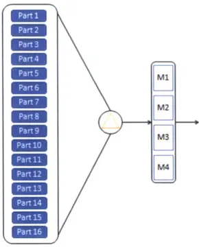
Figure 2. Parallel Machine Example

Figure 2 shows a parallel machine environment with four machines and sixteen jobs. All

machines in this example have the exact same capability to handle any part. The algorithm uses due dates and processing times to make decisions about machine assignments.

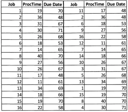
Job ProcTime Due Date Job ProcTime Due Date 1 19 70 11 17 48 2 36 48 2 36 48 3 31 67 6 18 53 4 30 71 9 27 56 5 26 68 16 22 58 6 18 53 12 11 61 7 14 65 7 14 65 8 40 70 14 18 66 9 27 56 10 26 67 10 26 67 3 31 67 11 17 48 5 26 68 12 11 61 13 34 69 13 34 69 1 19 70 14 18 66 15 19 70 15 19 70 8 40 70 16 22 58 4 30 71

Table 1. Example Job List

Table 1, above, shows the jobs and their pertinent information for machine assignment. The ProcTime column includes both the set-up time and run time for the jobs in this example. After the jobs are sorted by due date, the list will be used to assign the jobs to one of the four

caEM' m CM I2 M &=D ga d F-s am D I=m LM LIZEL a, umas N _

E~

m

i

mEE

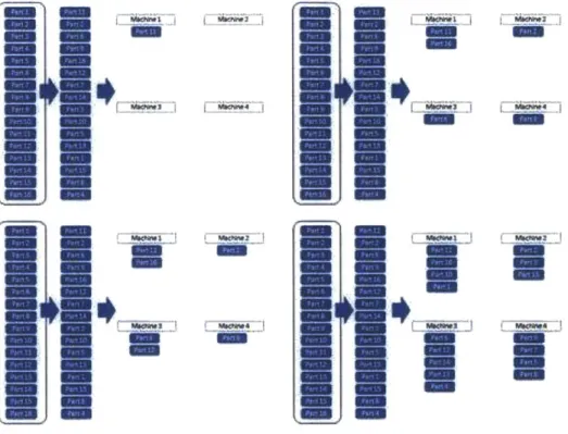
-M I M _

Figure 3. Job Assignment Process

Figure 3 shows the job assignments from the earliest due date sorted list in Table 2 in the four machine environment. The next

job

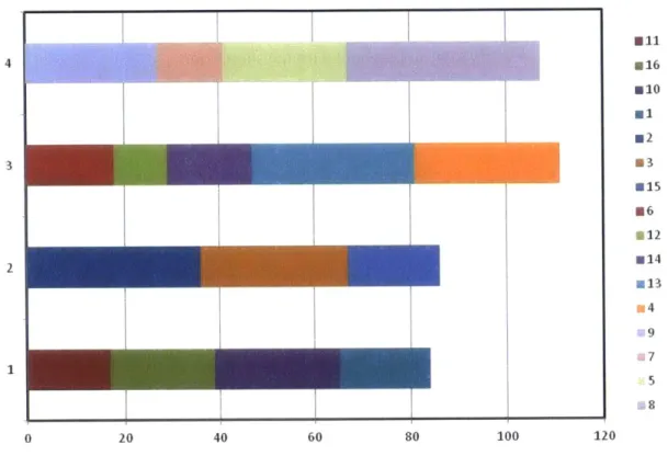
is assigned to the first open machine. Job 16 is assigned to machine I because it finishes first and job 12 is then assigned to machine 3. This process continues until all jobs are assigned. This machine assignment information and completion times are used to construct a Gantt chart.

El 4 .16 610 m2 W15 46 12 v14 2I 4 9 7 8 0 20 40 60 80 100 120

Figure 4. Gantt Chart for Earliest Due Date Example

4.2.3. Initial Results

Using the earliest due date to assign work to machines emulates the current practices on the shop floor. It produces feasible schedules that can be run by the machines and are at least as

good as the manual schedules. This method successtully automates scheduling, potentially

reducing the load across all supervisors by several hundred hours a week. While the approach does not produce optimal solutions, it is easy to implement give the current systems architecture.

4.3. Part Grouping

4.3.1. Motivation

Set-up times represent a significant percentage of the time that a part spends in the manufacturing process. The shop floor groups parts by set-up types in order to make the production process more efficient. The motivation behind this method is to fully capture the

savings from set-up reductions by incorporating part groupings into the earliest due date scheduling algorithm. The parts that use the same tooling and fixtures are grouped by taxonomies, which are currently kept in playbooks on the shop floor.

4.3.2. Methodology

This methodology builds on the earliest due date algorithm presented in the previous section by adding the ability to group parts with similar taxonomies. Parts with similar

taxonomies use the same fixtures and tooling, but there might be variation in the actual operation run. Again, we are examining the work queue that is present in front of a group of machines.

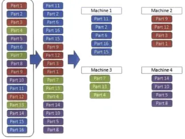
The algorithm first groups parts with similar taxonomies for the machine group. The jobs are then arranged by earliest due date inside the groupings. The groups are then sorted by due date using the earliest due date for the first job in the group. The first group is placed on the first open machine. The completion time for the group is the set-up for the first job and the processing time for all jobs in the group.

Machine 1 Machine 2 i

rt6MPachne3 Pachne4

Figure 5. Part Grouping

Fig-ure 5 shows a list of parts that are then grouped by taxonomy. There are four

taxonomly groups in this example. Parts eleven through fifteen on machine one are in group one, parts nine throug7h one on machine two are in group two, parts seveni through four on machine

three are in group three, and parts fourteen through eight on machine four are in group four. In this scenario, we saved twelve set-ups across all four machines.

4.3.3. Results

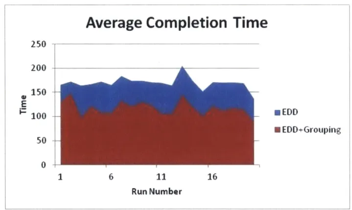
Simulations were used to compare the results of the part grouping and earliest due date method versus just the earliest due date method. The simulation consisted of twenty runs of thirty

job problems. The tool groups were assigned using a random number generator with a range

from one to eight. Due dates for the jobs ranged between forty-eight and seventy-two hours. Set up times in hours ranged between two and twenty. Run time in hours was between one and twenty. The simulation results showed a thirty percent reduction in the total run time of all machines in the group. No machine finished later using the part grouping method than the last machine using the earliest due date method.

Average Completion Time

E 250 200 150 100

s

EDD 0 EDD-1rOuingtc 50 0 6 11 16 Run Number

Figure 6. Set-up Time Reduction for Part Grouping 1

4.4. Wait Times 4.4.1. Motivation

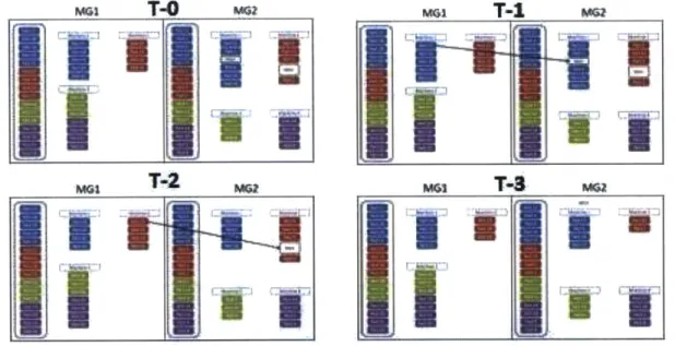
Supervisors will intentionally idle a machine because they know that a priority job is downstream and setting up the machine for a different job will delay the higher priority upstream work. This is an effort to prevent further tardiness of an already late job and generally does not cause a significant delay for the other jobs. The ability to add wait times is important to help

meet demand when a part close to yield fails quality inspection and another part needs to be accelerated. T-0

W

I

T-2 G_ -m C T-1

Figure 7. Supervisor's Wait Time Method

Figure 7 depicts the method for wait times as explained by a supervisor. The supervisor was trying to reduce the tardiness of a higher priority job that was several operations away by

allowing idle time in his machine group. Starting a lower priority job would occupy the machine when the higher priority job arrives and therefore cause a delay.

4.4.2. Methodology

The integer program was capable of solving the problem with optimal results in a minimal amount of time. It incorporated wait times for jobs that had higher priority because of their due date. This method also integrated the flexible job shop where earlier approaches were not able to. However, the model would have difficulty with the actual problem because there are

II

II

MG

I.

Ii

U

m

I

N44? ___

II.

.Ii*

I

I.

ii

'U.

I

significant number of non-machine activities where processing times are unknown and parts often exit the system to use outside resources.

4.4.3. Results

The integer program was capable of solving the problem with optimal results in a minimal amount of time. It incorporated wait times for jobs that had higher priority because of their due dates. This method also integrated the flexible job shop where earlier approaches were not able to. However, the model would have difficulty with the actual problem because there are

a significant number of non-machine activities where processing times are unknown and parts often exit the system to use outside resources.

4.5. Initial Conclusions

The three models discussed have strength and weakness for use as a short interval scheduling tool. The first two models use dispatching rules to schedule the jobs and are easier to implement with the current MRP system. Neither is an optimal solution and cannot simulate the entire factory. Neither model requires significant upkeep because the information is pulled directly from MRP data. The third model, which uses an integer program, has the capability to simulate the entire factory and produce optimal solutions, but is challenged by the problem size. This model is significantly harder to implement because of the number of variables, and because of the size and complexity of the shop.

5. Implementation

This chapter discusses the implementation of the tool, which includes what data the tool uses and how it simulates the plant, the dashboard, the adoption and rollout plan, and the results. Implementing a scheduling tool in an environment as complex as MCI is a serious undertaking because of the number of stakeholders involved.

5.1. Data Streams and Prediction of Part Flow

The three methods addressed in the previous chapter are able to schedule the queue of work for a group of parallel machines at a specific instance. These methods are not

interconnected and do not move work through the shop. In order to incorporate the

methodologies into a scheduling tool, we developed a method to simulate the movement of parts through the factory in order to build a schedule that would meet the three-day goal for each machine group.

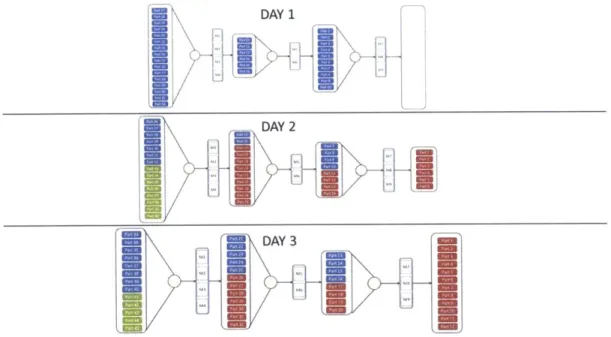
In order to solve this problem, we developed a second forecasting algorithm which would move completed jobs to the next queue. The scheduling algorithm would take all the work in the current day queue and schedule it. The forecasting algorithm would take all of the jobs

completed and using their routing, assign them to the next queue of the machine that performs the next operation. The scheduling algorithm schedules for day two using the jobs from the previous day that had not completed and the

jobs

just moved into the queue. This process is repeated to build out the schedule for three days while simulating the flow of jobs through the shop. The figure below shows how the part predictions advance the jobs across multiple days. The blue jobs represent all of the jobs currently in the queue, the red jobs are jobs completed the previous day, and the green jobs are jobs that are new to the system. This visual representation was useful in communicating the methodology of the prediction to the supervisors because they could see how the jobs would move.

DAY 1

E~EM

Figure 8 PaIPeito iga

There are several instances where

jobs

exit the system to enter an outside resource like a supplier. The

jobs

will reenter the system when they return. The prediction algorithm moves the

job

into a queue ibr these resources in order to provide visibility of when it will be available to send to the supplier. However, the scheduler will not be able to predict the

job

until it returns from a supplier and is placed into the current day queue.

5.2. Dashboard

The dashboard was developed to give the user the ability to interact with and change key parameters that would effect the scheduling algorithm. It provides a method for viewing the output of the scheduler. We identified that the user would need to be able to intel-act with the machine groups, part taxonomies, and output pacer charts. The dashboard for the tool was based on the architecture for a previous scheduling project.

5.2.1. Resource Editor

The machine grouping wizard in the dashboard gives the user the ability to build and edit the groups of parallel machines. It also gives the user the option to add or subtract a machine from the group for capacity reservations aiid allows planned downtime for maintenance to be

incorporated into the scheduler. This feature is important as new machines are added to the system and older machines are differentiated for specific parts.

5.2.2. Taxonomy

The Taxonomy tab lets the user group similar parts and operations for that machine group for the scheduler to use to reduce the number of set-ups. The user is able to select a part and then assign a taxonomy group for each operation. This taxonomy group uses the same tooling, fixture, and set-up for the machine. The majority of this information is available on the shop floor. This tool formalizes a method to capture this information so the most efficient schedule can be built. It will also incentivize efforts to use standard tooling and fixtures for common parts.

5.2.3. Pacer Charts

The pacer charts will provide a visual of the work that each machine needs to complete. It shows the set-up times for each job and the run time for each part. This allows the operator to pace his work flow. This tool will provide both the operator and the supervisor with a way to detect a problem during the operations. This will serve as an andon, signaling that there is a misalignment between the schedule and actual work. The supervisor and operator can then investigate the cause of the misalignment to determine the root cause. Currently, this is not possible, which is why the pacer tool is a critical niece of the implementation.

5.3. Adoption

The goal of the project was to not only provide a useful tool for scheduling, but also to motivate the shop floor to actually use the tool every day. Understanding the company as it relates to change would be critical to a successful adoption of the tool.

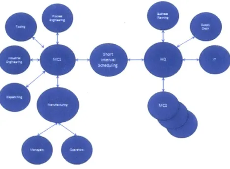
The initial step of developing the adoption plan was to conduct a stakeholder analysis to understand all of the key organizations involved and their relevant interests in the project. While short interval scheduling might seem to be limited in scope and confined to the manufacturing organization, it actually has many stakeholders across the entire enterprise. The key stakeholders were the operators, management, dispatching, tooling, industrial engineering, business planning, and IT. Figure 9 shows relationships between the various stakeholders of the project.

8e

Figure 9. Stake Holder M/ap

After conducting the stakeholder analysis, interviews were completed with each group to understand their position and begin to gain their buy-in. Three major themes about IT based manufacturing tools emerged from the interviews:

* they were excessively time consuming,

" they were not designed for the end user, and " they were not used by manufacturing.

These concerns were voiced by the supervisors, operators, and IT personnel respectively. These groups also had the strongest opinions about a tool. The supervisors and operators were most heavily invested in the tool's use. IT was most heavily invested in the tool's development and maintenance. The engagement strategies for each group are below.

* Supervisors

o Identify early adopters

o Use quick wins to establish credibility o Early adopters lead implementation

* Operators

o Engage during interface development o Communicate system benefits

o Integrate feedback and improvement system * IT

o Incorporate existing infrastructure o Demonstrate support of manufacturing o Quantify system improvements

In order to engage the supervisors during the development process, one supervisor from each area of the plant was identified as an early adopter and was used during the development of the model. A quick win with the supervisors would help build their confidence in the solution and make them advocates to both their operators and outside organizations like IT. An Excel and python prototype ran parallel to their process several mornings to show how the algorithm was making similar decisions to their own. This activity help build the confidence of the two early adopter supervisors in the scheduler. It also helped provide additional knowledge about the quirks existing in their individual areas, i.e. two machines are identical in the database but are not identical in reality, or jobs present in that area in the system were not actually present. These problems represented a significant amount of noise and required filtering to provide

improvement results. Quickly addressing this concerns built trust between the IT team, industrial engineers, and the supervisors.

These supervisors were also selected to lead the implementation because they were respected by their peers and could clearly communicate how the scheduler worked and how it improved the scheduling process, freeing up a significant amount of their time. This helped address the major concern that any tool would only increase the time requirements on the supervisors and the work would be non-value added. The message was better received coming from a peer than an outsider.

The major concern of the operators was that the interface with the system would not be designed with the end user in mind. The tool has three major end users, manufacturing

supervisors and operators, dispatchers, and tooling. Focus groups were used to determine what information needed to be displayed and the best way to present the information. This

engagement helped the operators feel like they were invested in the tool. There was also some concern from the operators that the tool would be used to punish non-performance. The communication plan addressed these concerns by addressing the adherence metric used to measure system performance and to identify misalignments between operations. Another key

message was that the schedule provided a clear goal for all areas to work towards, which was well received by the operators because it clearly defined the expectations of the day.

Using the manipulating and recombining tactics presented by Sonenshein, current infrastructure could provide all of the necessary information required by the scheduling tool, IT would only need to integrate these existing resources with the scheduling algorithm. The creative resource of existing resources reduces the downside if the tool happens to go unused. IT was

concerned about developing a tool that would not be used, so the two supervisors were brought in to articulate how the tool would save them significant time. This time savings alone justified the programmer hours needed to build the tool. The enthusiasm of the supervisors about the tool put a manufacturing face on the project and convinced the IT managers that a well-designed tool would in fact be used.

The deliberate approach for the adoption of the tool helped identify and mitigate many of the possible obstacles that the project faced. Engaging key stakeholders built consensus and alignment and ultimately fostered a sense of ownership in the project process.

5.4. Roll-out Plan

The roll-out planned to have two phases with a pilot and then full implementation. This method for implementation was selected because of the cultural challenges identified with change. The phased implementation assured that a quality solution would be delivered to the majority of the users. The early adopters for the pilot were comfortable working through the issues because they fully understood the impacts of the scheduling tool. The major objectives of the pilot were to validate both algorithms, debug the tool, define standard work and process flow and refine the user training program. The pilot was used to validate that the algorithm was working with the MRP system and with the part taxonomy database. Two areas of the plant that had sequential operations were used during the pilot to test the forecasting algorithm. During the pilot, the training program for the tool was refined for the operators, supervisors, and dispatchers.

Tool~ing

__

1l

k R'd i 'i i I~ dar

Figure 10. New Scheduling Process

During the pilot, a new process flow was mapped and is depicted above. The process reduced the number of handoffis as compared to the initial process depicted in Figure 1. These changes to streamline the flow reduced the ambiguity about which schedule was correct. While designing the new process, standard work was created to identify who did what work. This eliminated confusion about responsibilities that were present in the previous system. The table below shows how tasks were assigned to different functions. Standard work was then developed for each of the sample tasks.

Dispatching Identify orders on hold

Dispatching Order Day 3 tooling

Dispatching Load shop according to build plan

Tooling Deliver Day 1 tooling

Supervisor Validate work in area

Supervisor Place non-workable orders on hold Table 2. Example Standard Work Tasks

During the full implementation, training was conducted with all of the involved workers to introduce the new process and standard work. Integrated simulations were conducted with the entire support group so that they could see the work flow. Supervisors and operators from the pilot areas socialized the tool with the new areas. Industrial engineering provided assistance by placing orders on hold and collecting part family information and entering it into the central database. This approach led to acceptance of the new tool because each function was able to see overall system improvement.

5.5. Metrics

Schedule adherence is the primary metric used to evaluate performance of operators while using the tool. Schedule adherence monitors how closely the operator is able to build to the schedule. It will be measured by dividing the number of jobs completed per day by the number of jobs scheduled per the schedule. Using this metric will identify problems in the manufacturing system because low adherence will be investigated to determine the root cause of the problem. The schedule adherence metric might be lower than expected for several reasons to include:

" unscheduled machine maintenance, " incorrect part routing,

* incorrect scheduling standard, waiting on tooling, or * waiting on work.

An adjusted schedule adherence metric will allow us to gauge the performance of the individual operators. The metric will be adjusted for situations like those discussed above that are outside the control of the operators. This holds the operator accountable for only the work he is able to build.

Change in monthly shortages is the metric used to judge the overall performance of the scheduling algorithm. The scheduler should improve the plant positions on shortages because it will be building to due dates.

In previous sections, the predicted results of the scheduler were presented. During the

implementation, data was collected in order to see how the actual results compared to both the predicted results and the current state.

Supervisor Hours Spent Scheduling

350 300 250 0 200 150 Prior to Scheduler 100 a After Scheduler 50 0 1 2 3 4 5 6 7 8 9 10 Week

Figure 11. Supervisor's hours spent scheduling

Initial predictions indicated that the scheduler was expected to save around 300 hours of supervisors' time during a week. A survey was used to collect information about the number of hours supervisors spent scheduling for ten weeks before and after the

scheduler was implemented. Prior to the scheduler, supervisors were spending on average 296 hours per week on scheduling. After the scheduler was implemented the number of hours spent on scheduling dropped to an average of 37 hours per week. This

did not go to zero as expected because supervisors still spent time dealing with

exceptions or correcting incorrect data that was pulled into the scheduler from one of the data sources. I expect that over time, as the quality of the data used by the scheduling algorithm improves, the number of hours spent scheduling will continue to decrease. The reduction in supervisor hours is nearly 88% and this represents significant savings in valuable time the supervisors call spend completing other tasks.

Schedule Adherence

100 90 80 70 60 50 c 40 30 20 10 0 1 2 3 4 5 6 7 8 9 10 Week

Figure 12. Schedule Adherence

Data For schedule adherence was collected for ten weeks with the average adherence for the ten weeks at 82% (, which was better than the target of 80o during the initial adoption. As noted earlier in the section about schedule adherence, there are several reasons why the operator would not be able to build to the schedule that are beyond his control. During the ten wccks of the data collection, the majority of reasons for deviation from the schedule \\ere:

* incorrect routing,

* unexpected downtime,

* waiting on toolingy, and

* vaiting on work.

As these issues are addressed the deviations from the schedule will decrease and the deviations From problems outside the operators' control should significantly decrease.

Schedule Adherence Deviations

Sol'

3 4 5 6 Weeks 7 8 9 10 * Incorrect Routing Unexpected Downtime m Waiting on Tooling m WaIting on Work

Figure 13. Schedule Adherence Deviations

Figure 13 shows the causes of deviation from the schedule by the number of operations missed with the primary driver being unexpected machine down time. This is unsurprising since the model does not include a method for accounting for unexpected downtime. An improvement to the model could incorporate a probabilistic model using historical data on machine downtime to predict whether or not a machine is expected to be operational. The other three drivers are expected to continue to decrease overtime as the quality of the data improves, specifically data regarding routing and part taxonomies, and as interactions between the functions improves.

350 300 250 200 150 100 50 0 . 0 I 1 2

Actual Savings Using Part Grouping

7000 6000 4000 0 M EDD 1000 0 1 2 3 4 5 6 7 8 9 10 Week

Figure 14. Actual Set-up Time Reduction

The chart above shows the actual number of hours saved using part grouping for ten weeks. The gap between the EDD and EDD + Grouping represents the number of hours saved. It was calculated using the full set-up and run time for all parts and then the set-up for all parts where a set-up was not required because they were grouped. The average hours saved over the ten weeks was 940, which is a 15.7% reduction in production time. The predicted savings from the

simulation was around 30% and the reason for the difference between the actual and predicted saving is incomplete taxonomy data for the grouping function. As the remaining taxonomy data

is incorporated in the dataset, the set-up time reduction saving should increase towards the predicted percentage.

6. Conclusion

6.1. Key Findings and Recommendations

During the implementation, the tool demonstrated that it significantly reduces the number of hours that supervisors spend scheduling, it provides a method to synchronize dispatch and tool production to support manufacturing, and it reduces the number of set-ups of a machine, which better utilizes manufacturing capacity.

One of the other benefits of the tool is highlighting otherwise unapparent data inconsistencies and allowing for them to be addressed. These data inconsistencies included bad part routings, wrong tooling or fixtures, and incorrect standards for span time. These issues had previously been handled directly by operators with the updated information never making it to planner or other critical support personnel. Correcting these inconsistencies help overall system

performance by providing better information to master scheduling, tooling, and other key support functions.

The part taxonomy dataset was not complete and the algorithm could not effectively group all of the similar parts. Effort needs to be spent to collect and group all of the parts by common fixtures and tooling. Completely building out the part taxonomy data will greatly improve the efficiency of the system by reducing unnecessary set-ups.

The scheduler does not handle steps in the manufacturing process that are process labor based. The scheduler tells these activities when material will arrive but does not predict material coming out of this activity for a downstream machine. Additional effort needs to be spent to model the process labor based activities for the scheduler. Until then average times for these activities can be used to predict work for downstream machines.

Aircraft Company X has other manufacturing sites that can use the scheduler. The process for utilizing the scheduler in the other facilities would be similar to the roll out at MCL. The resources for each facility would need to be built and the tooling information collected. The other facilities have similar work and can benefit from the scheduler.

6.2. Opportunities for Further Research

There are several opportunities for additional research from the topics presented in this thesis. The infrastructure and datasets for the tool have been built and the tool is using

dispatching rules to schedule and predict production of parts in the plant. There is an opportunity to improve the optimization engine that the scheduling tool is using. Since the goal of this project was automation of short interval scheduling, optimality of the solution was not a primary

focus. Now that the schedule is automated and the datasets are built, additional work can focus on producing an optimal schedule. An integer program could be used to solve for tardiness for each of the parallel machine groups to allow for the fluidity of the current schedule or an optimization of an entire production area could be done with an increased time hoizon.

Additional research could also could be done to customize the scheduler for other production sites at ACX. Since the production flows at these sites differ from MCI, different approaches including integer programming could be used to solve the scheduling problem. This work could include incorporating non-machine resources into the scheduling tool. These activities are based on the number of people participating in the work. There are also many process based activities that could be modelled to improve the scheduler.

Appendix 1: Sample Problem

Group Number Number of Machines Group Set-up Time Run Time Group Set-up Time Run Time Group Set-up Time Run Time Group Set-up Time Run Time Group Set-up Time Run Time Group Set-up Time Run Time Group Set-up Time Run Time Group Set-up Time Run Time Group Set-up Time Run Time Group Set-up Time Run Time 1 4 Job 1 1 11 1 Job 2 1 4 5 Job 3 1 7 2 Job 4 1 10 7 Job 5 2 9 1 Job 6 1 10 3 Job 7 1 12 4 Job 8 2 8 2 Job 9 1 6 15 Job 10 2 5 4 Machine 2 1 2 7 11 3 6 12 2 12 13 2 6 6 3 4 11 2 12 10 3 9 Groups 3 4 4 8 6 4 7 12 4 10 17 3 10 7 4 7 16 4 6 15 2 7 17 10 3 10 6 2 11 1 1 4 4 4 5 14 4 12 9 4 8 18 4 5 5 2 Total Time 3 11 11 5 11 15 5 12 6 5 11 6 5 5 2 37 29 28 44 41 38 37 26 25 30 28 28 37 37 27 31 38 36 24 38 4 9 6 5 4 9 5 11 13 V V 3 9 11 3 7 12 5 8 8

References

Balas, E., Glover, F., & Zionts, S. (1965). An Additive Algorithm for Solving Linear Programs with Zero-One Variables. Operations Research, 517-549.

Graves, S. C., Meal, H. C., Stefek, D., & Zeghmi, A. H. (1983). Scheduling of Re-Entrant Flow

Shops. Journal of Operations Management, 197-207.

Honeywell Aerospace. (2016, February 19). Honeywell Forecasts. Retrieved from Honeywell Website: https://honeywel1.com/News/Pages/Honeywell-Forecasts-Steady-Global-Helicopter-Demand-For-Next-Five-Years.aspx

Kalir, A., Zorea, Y., Pridor, A., & Bregman, L. (2013). On the complexity of short-term

production planningand the near-optimality of a sequential assignment problem heuristic approach. Computers & Industrial Engineering, 537-543.

Montazeri, M., & Van Wassenhove, L. (1990). Analysis of scheduling rules for an FMS.

,International Journal of Production Research, 785-802.

Pinedo, M. (2012). Scheduling: Theory, Algorithms, and Systems. New York: Springer.

Sonenshein, S. (2014). How Organizations Forster the Creative Use of Resources. Acedemy of

Management Journal, 814-848.

Spear, S. (2009). The High Velocity Edge. New York: McGrawHill.

The Economist. (2015, July 25). Rotors Slayed. Retrieved from The Economist: http://www.economist.com/node/21659752/print