The MIT Faculty has made this article openly available.
Please share
how this access benefits you. Your story matters.
Citation
Fischell, Erin Marie and Henrik Schmidt. "Autonomous assessment
of seabed ripple geometry from bistatic acoustic scattering data."
Proceedings of the Institute of Acoustics, 7-9 September, 2015,
Bath, United Kingdom, Institute of Acoustics, 2015.
As Published
http://www.proceedings.com/27961.html
Publisher
Institute of Acoustics
Version
Author's final manuscript
Citable link
http://hdl.handle.net/1721.1/109735
Terms of Use
Creative Commons Attribution-Noncommercial-Share Alike
Detailed Terms
http://creativecommons.org/licenses/by-nc-sa/4.0/
AUTONOMOUS ASSESSMENT OF SEABED RIPPLE
GEOMETRY FROM BISTATIC ACOUSTIC SCATTERING
DATA
EM Fischell Massachusetts Institute of Technology, Cambridge, Massachusetts, USA H Schmidt Massachusetts Institute of Technology, Cambridge, Massachusetts, USA
1
INTRODUCTION
One of the greatest sources of interference in the acoustic scattered fields from seabed targets is bottom scattering. Directional sand ripples in particular produce three-dimensional scattering radiation patterns when insonified that distort measured scattering fields from aspect-dependent targets. These bistatic scattered fields are impacted by the topography of the ripple field, such as anisotropic angle relative to the acoustic source and ripple geometry.
This paper describes a method for estimation of sand ripple field parameters with data from Autonomous Underwater Vehicle (AUV) sampling of the bistatic scattered acoustic field that results from insonification of the seabed with a fixed acoustic source. Background on sand ripple
scattering is first reviewed and simulation results are shown illustrating differences in scattered field results based on various parameters. The Support Vector Machine (SVM) regression methodology used for parameter estimation is then presented. Finally, the results for estimation of anisotropy angle, height and major correlation length are described based on simulation and the conclusions and suggestions for future work are stated.
2
BACKGROUND
2.1 Prior Work
Modeling of acoustic scattered fields from seabed ripple fields has been explored in several different papers. Schmidt and Lee1 described the development of an anisotropic ripple field scattering
simulation module, used here to explore the estimation of bottom roughness using bistatic data. Williams2 constructed a model for forward scattering and compared models to real data in the
forward scattering direction. Others have used acoustic data from various sources to estimate seabed parameters. For example, multibeam backscatter data have been used to determine seabed types and parameters using techniques including Neural Networks 3,4, and backscatter data
have been used to estimate bottom properties such as composition, spectral scattering coefficient and surface height power distribution5,6,7. Inversion techniques for estimation of seabed roughness
have also been explored8,9. Several techniques also exist for eliminating the rough interface
scattering noise from sidescan sonar data10.
These techniques utilize backscatter strength or propagation information rather than directional features that show up in the bistatic scattering field. This paper describes how more complex attributes of the three dimensional bistatic scattered field could be exploited in the estimation of bottom characteristics by insonifying a region of ocean bottom using an acoustic source and collecting acoustic data using an AUV fitted with a hydrophone array.
2.2 Simulation Studies
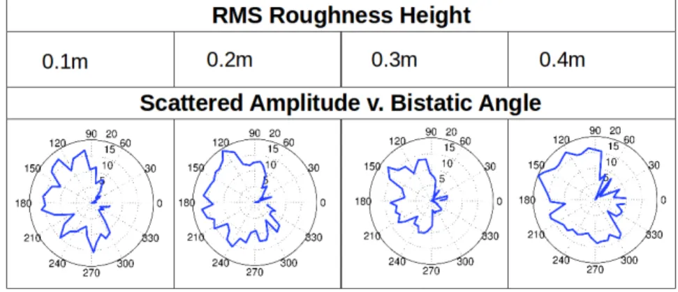
Simulation studies can be used to show how different ripple geometries affect the bistatic acoustic scattered field. In these simulations, some parameters of interest for the ripple field include the root
mean squared (RMS) roughness height √σ2, the major and minor correlation lengths of the field (C L1
and CL2) and the anisotropy direction of the field relative to the acoustic source (γ). These factors
cause different types of variation in the relationship between bistatic angle and scattered field amplitude. Figure 1 shows the mean scattering field amplitudes at all bistatic angles for varying values of RMS roughness height √σ2, Figure 2 shows the mean scattering field amplitudes for
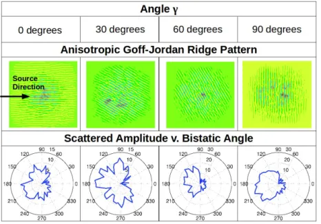
different values of major correlation length, and Figure 3 shows the mean scattering field amplitudes for different values of anisotropy angle γ.
Figure 1: Mean scattered amplitude versus bistatic angle for different values of RMS roughness height.
Figure 2: Mean scattered amplitude versus bistatic angle for different values of major correlation length.
3
METHODOLOGY
The goal of this research is to produce a set of algorithms and processes to estimate properties of sand ripple fields using AUVs without prior knowledge of the environment. This information could be used to enhance performance of bistatic target detection, localization and classification in inaccessible areas.
The basic configuration for this method is illustrated in Figure 4. A source, fixed relative to the bottom patch, insonifies a region on the bottom and an AUV samples the resulting scattered acoustic field. A model is trained using a set of example vectors mapping scattering amplitudes from a comprehensive data set to sampling location along an AUV path. This model is then used in real time by a vehicle to estimate the sand ripple field's properties of interest, √σ2, γ and C
L1, based
on scattering amplitude data.
Figure 3: Mean scattered amplitude versus bistatic angle for different values of anisotropy angle.
Figure 4: Schematic on the use of an AUV for estimation of ripple field parameters using sampled bistatic acoustic scattered field data. A fixed source insonifies a patch on the bottom using a 1kHz signal, an AUV samples the resulting scattered field and uses the collected amplitude data to estimate the anisotropy angle of ripple field.
3.1 Data
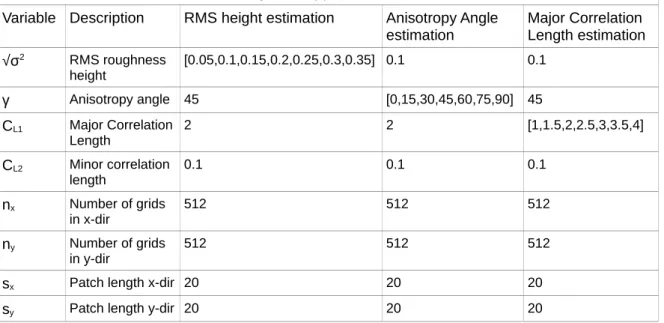
Because real 3D bistatic scattered field data for varying sand ripple topologies was unavailable, simulated data was used to develop and test the regression methods discussed in this paper. Scattered fields were modeled using the OASES-SCATT acoustic simulation package with Goff-Jordan anisotropic power spectra 1,11. Table 1 shows the parameters used for each of the three
regression tests: for estimating RMS roughness height, the major correlation length, and the anisotropy angle. For all simulations, the source is modeled as 1kHz, located at 10m depth and
100m from the patch being insonified on the bottom. The environment is modeled as a waveguide, with an air layer, a 30m deep water layer, and a sand bottom modeled as a fluid halfspace.
Table 1: Parameters used for simulating sand ripple bistatic scattered fields in OASES-SCATT. Variable Description RMS height estimation Anisotropy Angle
estimation Major Correlation Length estimation √σ2 RMS roughness height [0.05,0.1,0.15,0.2,0.25,0.3,0.35] 0.1 0.1 γ Anisotropy angle 45 [0,15,30,45,60,75,90] 45 CL1 Major Correlation Length 2 2 [1,1.5,2,2.5,3,3.5,4] CL2 Minor correlation length 0.1 0.1 0.1 nx Number of grids in x-dir 512 512 512 ny Number of grids in y-dir 512 512 512
sx Patch length x-dir 20 20 20
sy Patch length y-dir 20 20 20
3.2 Machine learning regression for parameter estimation
A supervised machine learning technique called support vector machine (SVM) regression was selected to perform the parameter estimation. First, the simulated 3D bistatic data sets were broken into randomly selected example vectors. Each example vector represents the scattering amplitudes collected along some AUV path through the field at depths of 5m to 15m and ranges to the center of the insonified patch of bottom of 20m to 50m. Independent training, validation, and test sets of these example vectors were generated from the simulated bistatic data sets. 4000 example paths were used for training, 2000 for validation and 2000 for testing. Since there are seven scattered fields sampled by each path, the training set consisted of 32000 examples, the validation and test sets each consisted of 14000 example vectors.
The example vectors represent the data to the machine learner as a sequence of feature-value pairs. The feature number indicates where in the bistatic scattered field an acoustic amplitude was collected, with the feature number Fs representing the azimuthal bin number based on the sample's
angle relative to the source-target line, θs, and a step size in bistatic angle, Δθ. Figure 5 shows how
this mapping occurs. For example, if an acoustic sample were collected at a bistatic angle of 7 degrees, and the bin size were 15 degrees, the acoustic sample would be mapped to Fs = 1. When
multiple samples were collected from the same feature, the median amplitude was taken.
3.2.1 Training and model selection
SVM regression was used to create a model from the set of training examples. SVM regression works by maximizing the minimum distance from the normal regression function to the set of training vectors. This training results in regression models that estimate parameter values based on new data represented in the same feature space. A good description of SVM regression can be found in Vapnik12.
SVM model parameters were selected using a validation set of example vectors. The validation set was independent of the data set used for generation of the SVM models and independent of the test set used to assess the model performance.
3.2.2 Analysis
Test sets, independent of training and validation data sets, were used to assess the performance of the trained models for each ripple field characteristic. Each test example represents a certain sampling by the AUV of the scattered field. The trained model was used to estimate the parameter of interest from each test example. The difference between the true and estimated parameter was used to assess the performance of the model. For each regression set, the same AUV sampling was conducted for all parameter values. For example, in the estimation of anisotropy angle, the test set consisted of example vectors that sampled the same points in the scattered fields of the 7 angles being estimated.
3.3 Real-time parameter estimation
The high fidelity Laboratory for Autonomous Marine Sensing System (LAMSS) MOOS-IvP13
simulation environment, which includes physics-based vehicle dynamics, environmental parameters and acoustic simulation, was used to demonstrate real-time regression on a virtual vehicle. The high-fidelity acoustic simulation includes interfaces to BELLHOP14 and OASES-SCATT11. In
simulation studies used for bottom topography estimation, a simulated version of the LAMSS vehicle Unicorn with a 16 element nose array at 0.05m spacing was deployed in a virtual ocean in 30m water depth off of the coast of Massachusetts. An acoustic simulator was developed to simulate acoustic arrivals, including multipath. This application used ray tracing models produced by BELLHOP to produce a time series across a simulated array. The time series included arrivals due to the direct blast from the source, source-target-vehicle arrivals and multipath with up to 3 bounces. Another process took in that time series and output an estimated amplitude for the insonified patch of bottom. Once the signal processing chain completed, an OASES-SCATT interfacing program published the scattered amplitude for the current location and geometry of the vehicle, source, and target or bottom patch based on the simulation model. An SVM model was specified to the SVM interface application, which ran real time regression on amplitude data as it was collected by the simulated AUV, updating estimated anisotropy angle until a specified confidence threshold was reached.
4
RESULTS
Three models were trained using the training set: a model for estimating the RMS roughness height of the ripple field, a model for estimating the major correlation length of the ripple field, and a model for estimating the anisotropic angle of the ripple field. The validation set was used to select the value for the complexity-accuracy tradeoff variable in the SVM model. The final models were tested using the test data sets and the results are shown below. All of the tested SVM models used linear kernels.
4.1 RMS roughness height estimation
Simulated scattered fields were created for roughness heights varying from 0.05m to 0.35m. The values of all other ripple field parameters were kept constant. The fields were then randomly sampled into independent data sets that represented what an AUV would sample while circling the insonified roughness patch. The training and validation sets were used to select the SVM
regression model, and roughness heights were then estimated for the test set.
The results showed that for the single frequency tested, the trained model was not effective at predicting the roughness height of the sand ripple field in the test set. Figure 1 shows why this may be the case: variation in the height of the sand ripple field mostly produces a change in the
magnitude of the radiation pattern but does not affect the locations of maxima pattern as much as changes in CL1 or γ. This means that the simulated AUV sampling likely does not produce enough
of a signal to compete with the noise in the data. Looking at a wider range of frequencies might provide a better basis for estimation of this parameter.
4.2 Sand ripple field major correlation length estimation
To test if CL1 could be predicted using an SVM regression model, simulated scattered fields were
created for CL1 varying from 1 to 4 meters. CL2 (minor correlation length) was fixed at 0.1m. The
same procedure was then followed for creating example vectors and training the regression model. The model was used to estimate the CL1 of the example vectors in the test set. All examples
represent 10 minutes of data collection by an AUV.
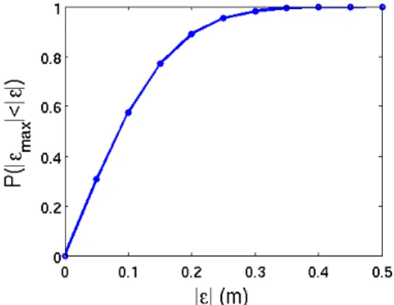
Figure 6: P(|εmax|<|ε|), calculated by finding the percentage of paths that resulted in less than ε
degrees error from regression of the test set.
The regression model was highly effective at predicting this length in the test set. Figure 6 shows a plot of the probability that a given new example vector (i.e. set of data collected by an AUV on some path around the insonified path) will have an error of less than ε meters maximum error, P(|εmax|<|ε|),
where ε is the estimation error variable in meters and εmax is the maximum regression estimation
error based on data collected on along the same path through the scattered fields from the seven sand ripple fields with different ratios. This plot shows that all example vectors resulted in an error of less than 0.5 meters, and that the estimate of major correlation length will have an error of less than 0.25m with a confidence of 95%.
4.3 Anisotropy angle estimation
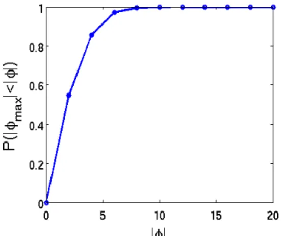
The model was created using simulation data for anisotropy angles of 0 to 90 degrees in 15 degree increments. The test set was used to assess the validity of the final selected model. Figure 7 shows a plot of the probability that a path will have less than φ degrees maximum error, P(|φmax|<|φ|),
error based on data collected on along the same path through the scattered fields from the seven anisotropy angles. These probabilities were calculated by finding the percentage of paths in the test set that had a regression estimation error of less than |φ| degrees. These results show that the model was highly successful in estimating anisotropy angle in this data set, with 100% of paths resulting in a maximum estimation error |φmax| of less than 10o and 95% showing a maximum error of
less than 6o. The test examples contain data from 600 samples, so this indicates that with 10
minutes of data collection around the insonified bottom patch, it is possible to get less than 6o error
with greater than 95% confidence.
Figure 7: P(|φmax|<|φ|), calculated by finding the percentage of paths that resulted in less than φ
degrees error from regression of the test set.
4.4 Real-time regression
The real-time regression processing was tested in virtual experiments in a MOOS-IvP simulation environment. The SVM model, feature space, and confidence model files were specified to a simulated vehicle. The simulated vehicle was commanded in a regression mission around a simulated rough patch 100m from the source. Acoustic data were emulated in real time using a combination of BELLHOP to simulate multipath arrivals on a virtual nose array and OASES-SCATT to simulate scattering amplitudes. The full processing chain ran in real time, coming up with progressive estimates of the anisotropy angle as the vehicle circled the target, until the regression confidence reached 95%. This was repeated with different simulated source locations and different bottom topographies. Running the processing chain in these simulations demonstrated the plausibility of real-time ripple field anisotropy estimation with onboard processing on an AUV
5
CONCUSIONS AND FUTURE WORK
This work shows the potential of using the bistatic scattered acoustic field from bottom ripples for parameter estimation. The generation of SVM regression models and use of those models in estimating the anisotropy angle and major correlation length of sand ripple fields in a real-time simulation environment was successfully demonstrated. There are several avenues of further work that should be pursued, given the success of this initial work. The results shown here are based on simulated scattered field data, but to confirm the viability of this methodology it should be tested using real acoustic data, either small scale or from full scale experiments. This work was also limited in that it looked at only one parameter at a time: further simulation experiments should be conducted to investigate the utility of this method with varying combinations of parameters. It would also be valuable to explore in simulation whether the same regression and confidence models could be successfully used with changes in environment, such as sound speed, depth, and bottom composition. There are additional parameters that could be investigated using this method, such as minor correlation length. Different frequencies and multiple frequencies should also be explored as
that might lead to more success estimating RMS roughness height. Overall, the simulation results show that this method has promise and warrants further investigation.
6
ACKNOWLEDGEMENTS
The authors would like to thank the LAMSS group at MIT for their continued research advice and assistance. This material is based on work supported by the National Science Foundation Graduate Research Fellowship under Grant Number 0645960, and by ONR Grant Numbers N00014-08-1-0011 and N00014-14-1-0214.
7
REFERENCES
1. H. Schmidt and J. Lee. Physics of 3-D scattering from rippled seabeds and buried targets in
shallow water. J. of the Acoust. Soc. of America 105, 1605–1617 (1999).
2. K.L. Williams and D.R. Jackson, Bistatic bottom scattering: model, experiments, and model/data comparison. J. of the Acoust. Soc. of America 103, 169–181 (1998).
3. C. Bishwajit and K. Haris. Seafloor roughness estimation employing bathymetric systems: An appraisal of the classification and characterization of high-frequency acoustic data. AIP Conf. Proc. 1495, 283–296 (2012).
4. Z. Huang, J. Siwabessy, S. Nichol, T. Anderson and B. Brooke. Predictive mapping of seabed cover types using angular response curves of multibeam backscatter data: Testing different feature analysis approaches. Continental Shelf Research, 61-62:12-22 (2013).
5. C.C. De, B. Chakraborty. Model-Based Acoustic Remote Sensing of Seafloor Characteristics. IEEE Trans. on Geoscience and Remote Sensing 49, 3868-3877 (2011).
6. H.M. Manik. Seabed Identification and Characterization Using Sonar. Advances in Acoustics & Vibration 2012, 1–5 (2012).
7. K.M. Becker. Effect of Various Surface-Height-Distribution Properties on Acoustic Backscattering Statistics. IEEE J. of Oceanic Eng. 29, 246-259 (2004).
8. S. E. Dosso, P.L. Nielsen and C.H. Harrison. Bayesian inversion of reverberation and
propagation data for geoacoustic and scattering parameters. J. of the Acoust. Soc. of Am. 125, 2867–2880 (2009).
9. G. Steininger, J. Dettmer, S.E. Dosso, C.W. Holland. Trans-dimensional joint inversion of seabed scattering and reflection data. J. of the Acoust. Soc. of Am. 133, 1347–1357 (2013). 10. H. Guanying, L. Qingwu, W. Min, F. Xijian and F. Xinnan. Side-scan sonar image despeckling
based on Bayesian estimation in curvelet domain. Chinese J. of Sci. Instrument 32, 170-177 (2011).
11. SCATT-OASES3D Users manual. Revision 2. [Online] Available:
http://lamss.mit.edu/lamss/docs/scatt manual.pdf (date last viewed 6/16/15).
12. V. N. Vapnik. The Nature of Statistical Learning Theory. Second Edition. Springer, New York, USA, 2000. Chapter 6, Methods of Function Estimation, pp 181-215.
13. M. Benjamin, H. Schmidt, P. Newman and J. Leonard. Nested Autonomy for Unmanned Marine Vehicles with MOOS-IvP. J. of Field Robotics 27, 834–875 (2010).
14. M. B. Porter. The BELLHOP Manual and Users Guide. Heat, Light, and Sound Research, Inc. La Jolla, CA, USA. January 31, 2011. [Online] Available: