Publisher’s version / Version de l'éditeur: Student Report, 2010-04-01
READ THESE TERMS AND CONDITIONS CAREFULLY BEFORE USING THIS WEBSITE. https://nrc-publications.canada.ca/eng/copyright
Vous avez des questions? Nous pouvons vous aider. Pour communiquer directement avec un auteur, consultez la
première page de la revue dans laquelle son article a été publié afin de trouver ses coordonnées. Si vous n’arrivez pas à les repérer, communiquez avec nous à [email protected].
Questions? Contact the NRC Publications Archive team at
[email protected]. If you wish to email the authors directly, please see the first page of the publication for their contact information.
NRC Publications Archive
Archives des publications du CNRC
For the publisher’s version, please access the DOI link below./ Pour consulter la version de l’éditeur, utilisez le lien DOI ci-dessous.
https://doi.org/10.4224/17519227
Access and use of this website and the material on it are subject to the Terms and Conditions set forth at
Development of high spatial resolution pressure sensor for model testing
Mostafa, Mohamad
https://publications-cnrc.canada.ca/fra/droits
L’accès à ce site Web et l’utilisation de son contenu sont assujettis aux conditions présentées dans le site LISEZ CES CONDITIONS ATTENTIVEMENT AVANT D’UTILISER CE SITE WEB.
NRC Publications Record / Notice d'Archives des publications de CNRC:
https://nrc-publications.canada.ca/eng/view/object/?id=30c9a36d-a995-40e8-8f2b-833106a4974c https://publications-cnrc.canada.ca/fra/voir/objet/?id=30c9a36d-a995-40e8-8f2b-833106a4974c
DOCUMENTATION PAGE REPORT NUMBER
SR-2010-12
NRC REPORT NUMBER DATE
April 2010
REPORT SECURITY CLASSIFICATION
Unclassified
DISTRIBUTION
Unlimited
TITLE
DEVELOPMENT OF HIGH SPATIAL RESOLUTION PRESSURE SENSOR FOR MODEL TESTING
AUTHOR (S)
Mohamad Mostafa
CORPORATE AUTHOR (S)/PERFORMING AGENCY (S)
Institute for Ocean Technology, National Research Council, St. John’s, NL
PUBLICATION
SPONSORING AGENCY(S)
IOT PROJECT NUMBER NRC FILE NUMBER
KEY WORDS
High spatial resolution, pressure sensor,prototype, ice,
PAGES iv, 17 FIGS. 11 TABLES 1 SUMMARY
This report describes the development of a high spatial resolution pressure sensor during my 4 months work-term at the Institute of Ocean Technology (IOT). Throughout this time period we focused on designing, building, and calibrating of the pressure sensor prototype that could be used for measuring ice pressure and its distribution during ice model testing at IOT’s ice tank.
ADDRESS National Research Council
Institute for Ocean Technology Arctic Avenue, P. O. Box 12093 St. John's, NL A1B 3T5
National Research Council Conseil national de recherches Canada Canada Institute for Ocean Institut des technologies
Technology océaniques
DEVELOPMENT OF HIGH SPATIAL RESOLUTION
PRESSURE SENSOR FOR MODEL TESTING
SR-2010-12
Mohamad Mostafa
TABLE OF CONTENTS
List of Tables ... iv
List of Figures ... iv
1.0 INTRODUCTION...1
2.0 OBJECTIVES ...1
3.0 DESIGN CONCEPT DESCRIPTION...2
4.0 PROTOTYPE BUILDING ...4
5.0 PROTOTYPE TESTING...6
6.0 DEVELOPING MATLAB SOFTWARE ...8
6.1 Finding Average intensity...8
6.2 Cropping Images ...10
6.3 Finding active pixels and the percentage of these pixels in the image ...11
6.4 Subtracting Two Images ...12
6.5 Finding active pixels and the percentage of these pixels in a directory of images ...12
7.0 IMAGE PROCESSING AND RESULTS...14
8.0 SUMMARY AND FUTURE WORK ...17
iv
LIST OF TABLES
Table 1: Results collected after several tests ...15
LIST OF FIGURES Figure 1: Ice drop testing with large-scale impact module (Gagnon, et al. 2009)...1
Figure 2: Schematic showing the function of the apparatus (Gagnon, 2008)...2
Figure 3: The above figure is an AutoCAD drawing of the different parts of the pressure sensor .3 Figure 4: One of the pressure films for the present pressure sensor ...4
Figure 5: The Two pressure films that were used in the testing of the prototype. Inflatable (left) and Non-slip tape (right)...4
Figure 6: Test apparatus and the power supply for LED lights ...5
Figure 7: Building procedure for the present pressure sensor ...5
Figure 8: Pressing on the pressure film (left) generate the image (right) on the mirror ...6
Figure 9: Increased Intensity of the contact area as a result of increased load ...7
Figure 10: Original Image (Left) and the cropped image (Right) ...8
DEVELOPMENT OF HIGH SPATIAL RESOLUTION PRESSURE SENSOR FOR MODEL TESTING
1.0 INTRODUCTION
This report describes the development of a high spatial resolution pressure sensor during my 4 months work-term at the Institute of Ocean Technology (IOT). Throughout this time period we focused on designing, building, and calibrating of the pressure sensor prototype that could be used for measuring ice pressure and its distribution during ice model testing at IOT’s ice tank.
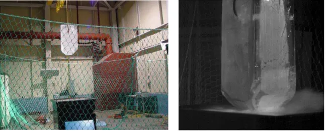
The concept of the present pressure sensor is the same as that of a large-scale impact module for bergy bit impact testing invented by Dr. Gagnon. For the large scale impact module can measure up to about 60 MPa whereas the present sensor could range up to 500 KPa for model testing. Fig 1 shows the ice drop testing with the large-scale impact module (Gagnon, et al. 2009)
Figure 1: Ice drop testing with large-scale impact module (Gagnon, et al. 2009)
2.0 OBJECTIVES
The objectives of this study are:
1. To design and build an apparatus to measure the pressure with high spatial resolution for ice model testing
2. To calibrate the pressure sensor with regard to light intensity 3. To develop Matlab Code to help image processing analysis
2
3.0 DESIGN CONCEPT DESCRIPTION
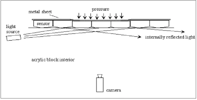
Fig 2 shows a schematic sketch for the principle of the pressure sensor. In this figure, the pressure sensor (film) is made of acrylic with slight curvature on the viewing side. When pressure is applied, this curvature is flattened and the amount of flatten area is captured by the camera with reflected lights. In other words, pressure is corresponding to the amount of flatten area.
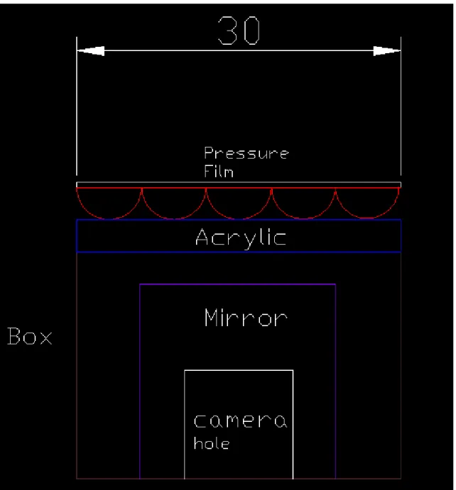
Figure 3: The above figure is an AutoCAD drawing of the different parts of the pressure sensor
Fig. 4 shows one of the pressure films for the present pressure sensor. Since acrylic has high Elastic Modulus, it wouldn’t be suitable for measuring low-pressure range from 50 ~ 500 Kpa. At this time, two different materials are used as the pressure film and both have a little dome shaped bumps that are the same role of curvature at the acrylic mentioned in the previous paragraph. Once pressure applied, these bumps are flattened (squeezed). Consequently the internal lights are frustrated and the flatten area can be clearly seen brightly. Details will be addressed in the Testing section.
4
Figure 4: One of the pressure films for the present pressure sensor
4.0 PROTOTYPE BUILDING
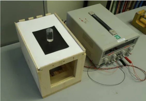
After series of solid works drawings and modifications of the concept, a final drawing with all the necessary dimensions was ready to be delivered to the workshop and eventually built in order to conduct the tests. The apparatus is a 20 x 21x 30 cm wooden box. For internal light, two LED strips are attached at each longer side of the top of the box. A 9mm acrylic block is used for a flat base: when pressure applied, the pressure film flattens against this acrylic block.
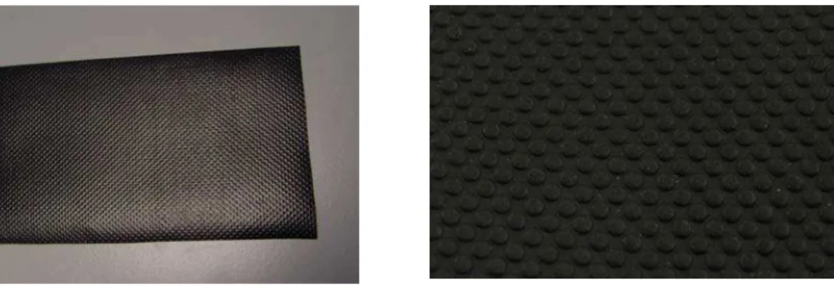
For the convenience, a mirror is used to view the pressured area and the camera is located outside of the box. A flat, 2.5cm of diameter cylinder shape indenter is used to exert pressure. In Fig. 5, two types of pressure films were used; an inflatable patch (normally used for inflatable boat repair) and a piece of Non-Slip Tape (model # 3418 from www. antisliptapeshop.com). Both materials have dome-shaped bumps and elasticity needed for the pressure measurement. Fig. 6 shows the test apparatus and power supply.
Figure 5: The Two pressure films that were used in the testing of the prototype. Inflatable (left) and Non-slip tape (right)
Figure 6: Test apparatus and the power supply for LED lights
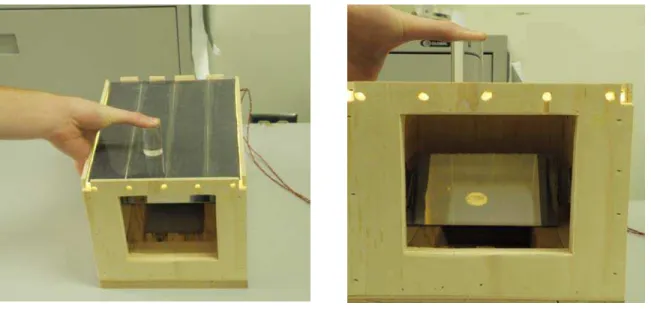
Fig. 7 shows the procedure for the sensor building. #1 shows the LED lights and mirror; #2 shows the acrylic block as the base; #3 shows the white thin paper to maximize the light reflection; #4 shows the pressure film (bumpy part should touch against acrylic base); and #5 shows the test apparatus with indenter.
Figure 7: Building procedure for the present pressure sensor
1
3
5
4 2
6
5.0 PROTOTYPE TESTING
After the prototype was built in the workshop, several tests were conducted for the calibration. For image capturing, a digital camera (DC09 with manual mode) was used. This is a preliminary stage to develop a calibration curve at the steady state but for dynamic pressure such as impact, a high-speed camera should be used. Both pressure films were used and a soft rubber sheet was attached on the tip of the indenter, which could help to distribute the load evenly.
One 2 kg-weight and four 5 kg-weights are used to exert the load on top of the indenter. A flat, round shaped piece (0.25kg) is placed between the indenter and weights to provide a stable condition for stacking up the weights. The apparatus was then covered by black vinyl to avoid outside light interfering in the result image.
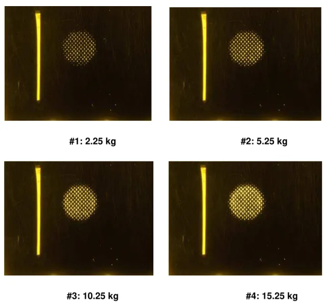
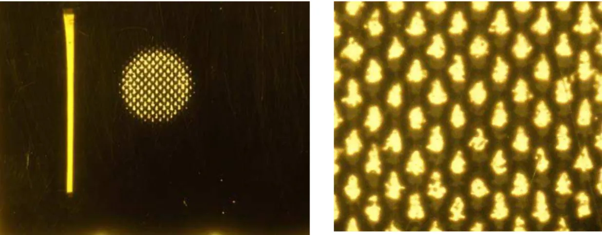
Fig. 8 shows the principle of the present pressure sensor and pressure area as an example. Fig. 9 shows the images taken from the calibration with inflatable patch. As seen in the figure, more pressure provides wider flatten area and more light intensity. It is noted that the strip in the left side of each picture is intended for an index of the light intensity but it didn’t use at this time.
#1: 2.25 kg #2: 5.25 kg
#3: 10.25 kg #4: 15.25 kg
#5: 20.25 kg
8
6.0 DEVELOPING MATLAB SOFTWARE
After the prototype was tested and several sets of images were taken, the next task was to develop a series of matlab code necessary for the image processing. First trial was to calculate the average intensity of whole images using”Threshold Intensity.” For the calibration purpose, any artificial effect such as applying threshold would be a risky. Therefore, the section of interest in the image was cropped and calculated the average intensity.
Fig. 10 shows the image taken by the camera (Left) and the cropped image (Right) using Matlab
Figure 10: Original Image (Left) and the cropped image (Right)
Below are Matlab files for intensity calculation and cropping.
6.1 Finding Average intensity
This program reads in one image of type (*.TIF) at a time in a certain directory. It transforms the image into a grey scale image and then goes through each pixel in the image of this number of rows and columns finds the intensity of this pixel and saves it in the variable total and then adds all these intensities and outputs the mean value of all these pixels.
function BlockImage(fileIn)
imInfo = imfinfo(fileIn); nRow = imInfo.Height;
nCol = imInfo.Width; total = 0; h = waitbar(0,'processing') ; Inc = 0; totalMean = 0; for i = 1:100:nRow for j = 1:100:nCol
if((nCol - j) > 100 & (nRow - i) > 100)
wrkIm1 = imread(fileIn,'PixelRegion', {[i i+100], [j j+100]}); wrkIm2= rgb2gray(wrkIm1); meanIm = mean(wrkIm2(:)); total = total+meanIm; Inc = Inc+1; end end
10
waitbar(i/nRow + 0.3);
end
fprintf('\n The Average Intensity is: ') totalMean = total/Inc
close all;
6.2 Cropping Images
The program crops an image of type (*.TIF). You input the coordinates of the region of interest. In the program here I inputted as an example values for the points present in column 670 and column 1814 and rows 1846 and 3020 of a region I needed to crop in an image. Cropping was used in the image analysis because you can eliminate all other factors that could interfere in calculating magnitudes of intensities. I cropped inside the area of contact and then calculated the brightness of that region for better results.
tifdir = dir('*.tif');
for file = {tifdir(:).name} file = char(file); I = imread(file);
I = I(670:1846,1814:3020,:);
imwrite(I,strcat(file(1:size(file,2)-4),'-crop.jpg')); end
6.3 Finding active pixels and the percentage of these pixels in the image
This program takes in an image of type (*.TIF) and then calculates the number of active pixels in that image and the percentage of the active pixels from the total number of pixels present in an image. Active pixels are the number of pixels that have intensity equal to or above a certain threshold frequency that I chose to input for the program. The threshold frequency varies between 1 and 100.
function BlockImage2(fileIn)
check = 0; while check==0
fileIn2 = input('\n please set the threshold, pick a number between 1 and 100 : ','s'); threshold = str2num(fileIn2);
if 0<threshold && threshold<101 check = 1;
end end
image = rgb2gray(imread(fileIn)); truthmat = image>threshold;
fprintf('\n Active pixels: ') active = sum(sum(truthmat)) fprintf('\n Percentage: ')
12
close all;
6.4 Subtracting Two Images
This program reads in an image two images each at a time and then transforms each of these images into a grey scale image subtracts both images and outputs the subtracted image in grey scale.
function Histogram(fileIn1,fileIn2) close all; image1 = imread(fileIn1); Image1 = rgb2gray(image1); figure(1), imagesc(Image1); colormap ('gray');
figure(2); imhist (Image1);
image2 = imread(fileIn2); Image2 = rgb2gray(image2); figure(3), imagesc(Image2); colormap ('gray');
figure(4); imhist (Image2);
figure(5), imagesc(imResult); colormap ('gray');
figure(6); imhist (imResult); imwrite(imResult,'Result.jpg')
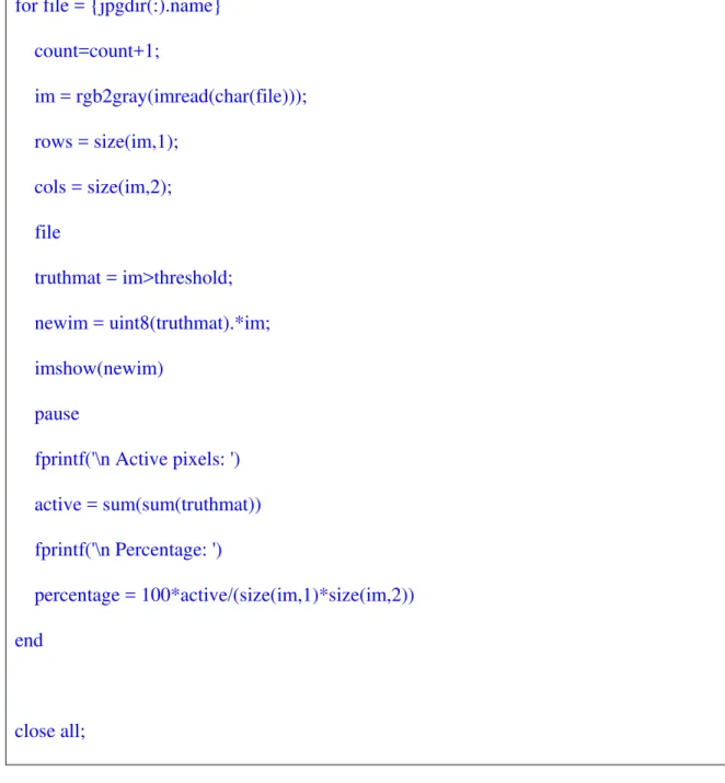
6.5 Finding active pixels and the percentage of these pixels in a directory of images
This program takes in a directory of images of type (*.jpg) and then calculates the number of active pixels in that image and the percentage of the active pixels from the total number of pixels present in an image. Active pixels are the number of pixels that have intensity equal to or above a certain threshold frequency that I chose to input for the program. The threshold frequency varies between 1 and 100.
function ImageSize(dirname) clc
check = 0; while check==0
fileIn2 = input('\n please set the threshold, pick a number between 1 and 100 : ','s'); threshold = str2num(fileIn2);
if 0<threshold && threshold<101 check = 1;
end end
count = 0;
14
for file = {jpgdir(:).name} count=count+1; im = rgb2gray(imread(char(file))); rows = size(im,1); cols = size(im,2); file truthmat = im>threshold; newim = uint8(truthmat).*im; imshow(newim) pause
fprintf('\n Active pixels: ') active = sum(sum(truthmat)) fprintf('\n Percentage: ')
percentage = 100*active/(size(im,1)*size(im,2)) end
close all;
7.0 IMAGE PROCESSING AND RESULTS
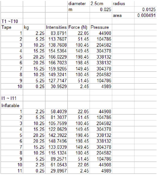
Table 1 shows the test matrix, pressure and calculated intensity from Matlab. In the table, T1~T10 indicates tests using non-slip Tape, and I1~I11 indicates tests using Inflatable patch as pressure film.
Table 1: Results collected after several tests
Fig. 11 shows the calibration graphs for both materials. At the same pressure, some discrepancies are found possibly because of delayed elastic response of pressure film or lack of stiffness of acrylic base for long time period of loading. For impact test, however, it wouldn’t be a problem. In this figure, inflatable patch would take more pressure since its intensity still shows a generous slope compared with that of non-slip tape.
16
Figure 11: Calibration Curves
Non-Slip Tape Inflatable
Intensity versus Pressure Curve
y = 348.17Ln(x) - 1394.8 0 50 100 150 200 250 300 350 400 0 20 40 60 80 100 120 140 160 Intensity Pressure (kpa) Series1 Log. (Series1)
Intensity versus Pressure Curve
y = 348.17Ln(x) - 1394.8 0 50 100 150 200 250 300 350 400 0 20 40 60 80 100 120 140 160 Intensity Pressure (kpa) Series1 Log. (Series1)
8.0 SUMMARY AND FUTURE WORK
From all that has come in this report, regarding the designing, building, testing, and the results, discussion and analysis, we can wrap up and say that the prototype pressure sensor apparatus was successfully designed, built and tested. The two pressure films were used and the pressure ranged from 50 kpa to 300 kpa. We noticed that the inflatable patch shows possibly large range of pressure based on the calibration
More testing needs to be done in the cold room with MTS machine to assess the temperature dependency of the pressure films because the model testing is going to be done in very cold temperature conditions. The MTS machine can provide both static and dynamic tests with much controlled condition including evenly distributed pressure for the indenter. The high-speed camera would be useful to acquire high quality images for highly dynamic tests such as ice impact.
9.0 REFERENCES
1) R. Gagnon, 2008, "A New Impact Panel to Study Bergy Bit/ Ship Collision," Proc. of the 19th IAHR International Symposium on Ice, Vancouver, British Columbia, Canada.