READ THESE TERMS AND CONDITIONS CAREFULLY BEFORE USING THIS WEBSITE. https://nrc-publications.canada.ca/eng/copyright
Vous avez des questions? Nous pouvons vous aider. Pour communiquer directement avec un auteur, consultez la
première page de la revue dans laquelle son article a été publié afin de trouver ses coordonnées. Si vous n’arrivez pas à les repérer, communiquez avec nous à [email protected].
Questions? Contact the NRC Publications Archive team at
[email protected]. If you wish to email the authors directly, please see the first page of the publication for their contact information.
NRC Publications Archive
Archives des publications du CNRC
Access and use of this website and the material on it are subject to the Terms and Conditions set forth at
Granular Computing Methods in Bioinformatics.
Valdés, Julio
https://publications-cnrc.canada.ca/fra/droits
L’accès à ce site Web et l’utilisation de son contenu sont assujettis aux conditions présentées dans le site LISEZ CES CONDITIONS ATTENTIVEMENT AVANT D’UTILISER CE SITE WEB.
NRC Publications Record / Notice d'Archives des publications de CNRC:
https://nrc-publications.canada.ca/eng/view/object/?id=9646e182-0f69-4eac-b511-b434f22b397e https://publications-cnrc.canada.ca/fra/voir/objet/?id=9646e182-0f69-4eac-b511-b434f22b397e
Granular Computing Methods in
Bioinformatics*
Valdés, J. 2007
* Handbook of Granular Computing. 2007. NRC 49337.
Copyright 2007 by
National Research Council of Canada
Permission is granted to quote short excerpts and to reproduce figures and tables from this report, provided that the source of such material is fully acknowledged.
!" #$!!
% & " % '#( ! ) * +#,+)#-, ..-/!001 2 * +#,+)#-, . $/!$#
#
The science of biology is very different from what it was two decades ago. It has become increasingly multidisciplinary, especially after the unprecedented changes introduced by the human genome project. This effort projected a new vision of biology as an
information science, thus making biologists, chemists, engineers, mathematicians, physicists and computer scientists cooperate in the development of mathematical and computational tools, as well as high throughput technologies. The entire field of biology is changing at an enormous rate, like a handful of other disciplines, exerting a boosting effect on the development of many existing technologies and inducing the creation of new ones. As a result, a large impact in human society is expected, with unforeseen consequences. In fact, many specialists and analysts believe that it will change forever the way in which modernity is understood.
Bioinformatics is an emerging and rapidly growing field for which no universally accepted definition may be found. In its broadest sense, it covers the use of computers to handle biological information, understood as the use of applied mathematics and
computer science to solve biological problems. Accordingly, it covers a large body of both theoretical and applied methods, with implications in medicine, biochemistry and many other fields in the life sciences domain. In the same sense, it involves many areas of mathematics (ranging from classical analysis and statistics, to probability theory, graph theory, etc.) and computer science, like automata theory and artificial intelligence, just to mention a few. Bioinformatics research considers general topics like systems biology or
modeling of evolution, and more specific ones like gene expression intensities, protein# protein interactions and other biological problems at the molecular scope. It is common to interpret bioinformatics as computational biology, however, they are recognized as
separate fields, although very related and overlaping. According to a Committee of the National Institute of Health, bioinformatics is oriented to the research, development, or application of computational tools and approaches for expanding the use of biological, medical, behavioral or health data, including those to acquire, store, organize, archive, analyze, or visualize such data; whereas computational biology focuses on the
development and application of data#analytical and theoretical methods, mathematical modeling and computational simulation techniques for the study of biological,
behavioral, and social systems. Regardless of whether bioinformatics is interpreted in a broad or narrow sense, a common denominator is the processing of large amounts of biologically#derived information, whether DNA sequences or breast X#rays.
Machine learning techniques oriented to bioinformatics in combination with other mathematical techniques (mostly from probability and statistics) are presented in [5]. Within bioinformatics there is a broad spectrum of problems requiring classification, discovery of relations, finding relevant variables, and many others, where granular computing approaches can be applied. Moreover, there are other issues like the
characterization and processing of uncertain information and the handling of incomplete data, where rough sets and fuzzy set approaches are particularly appropriate.
Granular computing provides a broad range of approaches for the analysis of biological data. Fuzzy and rough sets based techniques, in particular, are specially suited for handling uncertainties of different kinds. Moreover, within their framework many
powerful procedures have been developed for clustering, classification, feature selection and other important data mining tasks.The Rough Sets approach is particularly well suited to bioinformatics applications because of its ability to model from uncertain, approximate, and inconsistent data. The generated rule#models are easy to interpret by non#experts and they are also minimal in the sense of not using redundant attributes.
These techniques have been applied to a wide variety of biological problems and in more recent years to bioinformatics in the genomic and post#genomic era, but bioinformatics textbooks are not yet covering them regularly ([18], [7]).
In fact, the number of applications of granular computing techniques to bioinformatics is becoming large and is constantly increasing. It is impossible to cover all of these
developments here, therefore, only selected topics and examples are presented. The purpose of this chapter is to illustrate the scope, possibilities, and future, of the
application of granular computing approaches in the domain of modern bioinformatics.
$
*
62
(
Considered now as classical, are the tasks of storing, comparing, retrieving, analyzing, predicting and simulating the structure of biomolecules (including genetic material and proteins). Most large biological molecules are polymers, composed of ordered chains of simpler molecular modules (monomers) which can be joined together to form a single, larger macromolecule. Macromolecules can have specific informational content and/or chemical properties and the monomers in a given macromolecule of DNA or protein can be treated computationally as letters of an alphabet. In specific arrangements, they carry
messages or do work in a cell. This explains why, from the mathematical point of view, the interest was concentrated on sequence analysis.
After the completion of the Human Genome Project in 2003, the focus and priorities of bioinformatics started to change rapidly. Actually, they are constantly changing and several new streams within bioinformatics have emerged.
Genomics is the study of genes and their function. The genome is the entire set of hereditarily obtained instructions for building, running, and maintaining an organism, also used for passing life on to the next generation. The genome is made of a molecule called DNA and it contains genes, which are packaged in units called chromosomes and affect specific characteristics of the organism. In " multiple genomes are investigated for differences and similarities between the genes of different species. These studies have led to both specific conclusions about species and general considerations about evolution itself.
The identification of gene functions on a large scale and the discovery of their associations are of great importance, which is the purpose of . The set of proteins encoded by the genome is known as the proteome. The study of the proteome is the domain of which includes not only all the proteins in any given cell, but also the set of all protein forms and modifications, their interactions and the structural description of both the proteins and their higher#order complexes. The characterization of the many tens of thousands of proteins expressed in a given cell type at a given time involves the storage and processing of very large amounts of data. It is natural that artificial intelligence techniques, in general, and machine learning, in particular, find broad application in bioinformatics because of the need to speed up the
process of knowledge discovery. In this sense, data mining on the constantly growing bioinformatics databases is possibly the only way to achieve that goal.
One of the most important fields of modern bioinformatics where granular computing methods have a large potential and where successful applications have already been made is genomics; in particular, the analysis of DNA microarrays. DNA is the molecule that encodes genetic information. In Eukaryotes (all organisms except viruses, bacteria, and bluegreen algae), it is a double#stranded molecule held together by weak bonds between base pairs of nucleotides, namely adenine (A), guanine (G), cytosine (C), and thymine (T). Base pairs form between A and T and between G and C; thus the base sequence of each single strand can be obtained from that of the other. RNA is the molecule found in the nucleus and cytoplasm of cells; and it plays an important role in protein synthesis and other chemical activities of the cell. The structure of RNA is related to that of DNA. There are several RNA molecules: messenger RNA, transfer RNA, ribosomal RNA, and others.
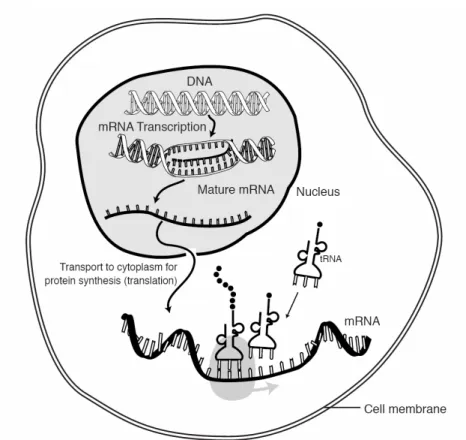
According to what is considered the Central Dogma of Biology (Fig. 1), DNA
experiences a process called which is the synthesis of an RNA copy from a sequence of DNA (a gene). From the RNA (actually, from the messenger RNA which is the one that serves as a template), a process called occurs, in which the genetic code carried by mRNA directs the synthesis of proteins from amino acids.
The cell determines through interactions among DNA, RNA, proteins, and other substances when and where genes will be activated and how much gene product (e.g. a protein) will be produced (the process is called gene regulation). In this process, genes are activated to produce the specific biological molecule encoded by them (gene expression) following very complex patterns of interactions. Traditionally, molecular biology experiments studied the behavior of an individual gene, thus obtaining a very limited amount of information and missing the more complex picture given by the interrelations of different genes and their functions.
Fig. 1. The Central Dogma of Biology. DNA leads to mRNA via transcription and then to Proteins via translation.
Recently, a new technology, called a DNA microarray, has been developed which has attracted tremendous interest among biologists. It allows the study of the behavior of large numbers of genes simultaneously, which potentially can cover the whole genome on a single chip. In this way, researchers can have a broad picture of the interactions among thousands of genes simultaneously ([60], [27], [39], [47]).
Complementary DNA (cDNA) is single#stranded DNA made in the laboratory from a messenger RNA template. It represents the parts of a gene that are expressed in a cell to produce a protein. Often it is used as a probe in the physical mapping of a chromosome. A DNA microarray is a glass slide with cloned cDNA in spots deposited on its surface at fixed locations according to a previously designed layout, in an operation usually
controlled by a robotic arm. Target mRNA from two different samples (test and control) are labeled with fluorescent dyes Cy5 and Cy3 (Red and Green respectively) which hybridize complementary DNA (cDNA). The mRNA degrades and the resulting mixture of cDNA from the test and control samples is applied to the microarray where some strand binds to their complementary probe strands after some time. The plate is washed in order to remove the strands which did not bind to any of the existing spots. Then the microarray is placed in a black box and scanned with red and green lasers producing two images where the intensity of each spot is proportional to the concentration of mRNA. For each spot a ratio of residual intensity of each of the dyes (i.e. removing the
background intensity of the corresponding dye) is computed. Thus, what is obtained is a measure of relative abundance between the two samples. Typically, many thousands of spots can be placed on a microarray surface and (even considering that in many
experimental designs duplicate spots are placed), thousands of genes can be studied simultaneously (Fig. 2).
One common use of microarrays is to determine which genes are activated and which genes are inhibited when two populations of cells are compared. This technology has been used in gene discovery, disease diagnosis, drug discovery (this field is called pharmacogenomics), toxicological research (the field of toxicogenomics) and other biomedical tasks.
Considering the costs involved in producing the microarrays and in conducting the experiments, the typical situation is that of having a relatively small number of objects (experiments) in comparison with the number of attributes describing each of them (genes). Depending on the particular situation, the objects may or may not have labels representing a disease, type of tumor, etc., leading to supervised or unsupervised problems involving classification and/or clustering.
$ # 7 88
There are several advantages of applying fuzzy logic to the analysis of gene expression data. Fuzzy logic inherently accounts for noise in the data, as they are understood as categories of a linguistic variable, with gradual boundaries in between. In
contradistinction with other algorithms like neural networks, support vector machines (SVM) or elaborated statistical procedures, fuzzy logic results can be communicated and understood with ease to domain experts (biologists, physicians, etc.). Also, fuzzy
procedures are computationally fast and efficient.
A relatively simple fuzzy logic approach for the analysis of gene expression data is that of [73], where expression data values were normalized to a [0,1] range and then fuzzified
by creating a linguistic variable with three categories (low, medium and high). Triangular membership functions were used for describing each category with cross# points at 0.5 membership values. Using yeast cell cycle expression data ([22]), triplets of gene expression values were defined (all taken at the same time point in the yeast growth cycle time series). A set of 9 rules assembled as a decision matrix were defined, each composed of an elementary conjunction of two attribute#value pairs corresponding to the first two genes of the triplet, and an attribute#value pair of the third gene in the triplet as the consequent (the value of a given cell in the decision matrix). The rules were
formulated with the assumption that the first conjunct is an activator gene and the second a repressor.
Then, an exhaustive search algorithm analyzed the triplets by applying the rules, and comparing the fuzzy predicted value for the third gene of the triplet. The squared
difference between the observed value and the defuzzified predicted value was computed and triplets with values smaller than a given threshold (0.015) were accepted. In addition, the variance of the number of hits corresponding to the cells in the decision matrix was computed and used as a second filtering criterion. Some very interesting triplets were found, and in particular those involving the HAP1 gene were followed up. By assembling the corresponding triplets, a regulatory network was assembled. The predicted network was highly consistent with the experimental data obtained from previous studies. Also, many of the most frequently found pairs of genes appeared to be biologically relevant. Genes are related in very complex ways and the discovery of these relations is an important goal of gene expression microarray data processing. From an unsupervised perspective, a classical approach has been looking for groups of genes which behave
similarly with respect to some predefined measure of similarity or distance using cluster analysis methods. Among them, hierarchical clustering and #means partitioning cluster are typically applied. However, the crisp nature of the partitions created by hierarchical methods where a similarity or distance value is used as the threshold for group separation is a great limitation. The same happens with #means methods, where the number of groups to construct has to be fixed in advance. This is especially problematic when analyzing large gene#expression datasets that are collected over many experimental conditions, when many of the genes are likely to be similarly expressed with different groups in response to different subsets of the experiments.
Fuzzy clustering ([57], [13], [14], [15]) on the other hand, facilitates the identification of overlapping groups of objects by allowing each element to belong to more than one group. The essential difference is that rather than the hard partitioning of standard k# means clustering, where genes belong to only a single cluster, fuzzy clustering considers each gene to be a member of every cluster, with a variable degree of membership. In classical #means clustering where the only parameter to specify is the desired number of clusters ( ). However, in fuzzy clustering yet another parameter ( ) must be indicated. It controls the fuzziness of the constructed partitions. When is 1 the result is a hard (crisp) partition like the one produced by classical #means. The larger the , the “fuzzier” the resulting partitions are going to be.
There are many variants of the fuzzy #means algorithms ([14], [32], [38]) and they have been applied to the analysis of gene expression data. An interesting modification to the Gath and Geva algorithm was introduced in [31] and used for exploring the conditional coregulation in yeast gene expression data. The algorithm was modified in two ways:
three successive cycles of fuzzy k#means clustering are performed, with the second and third rounds of clustering operating on subsets of the data; each clustering cycle is initialized by seeding prototype centroids with the eigen vectors identified by Principal Component Analysis of the respective dataset (this is done in order to attenuate the impact of random initialization on the results).
The first round of clustering is initialized by defining k/3 prototype centroids (where k is the total number of clusters and 3 is the number of clustering cycles) as the most
informative k/3 eigen vectors identified by PCA of the input dataset. In the subsequent steps the prototype centroids are refined by assigning to each gene a membership to each of the prototype centroids, based on the Pearson correlation between the gene’s
expression pattern and the given centroid. Then the centroids are recalculated as the weighted mean of all of the gene#expression patterns in the corresponding group, where each gene’s weight is proportionate to its membership in the given cluster. The process is iterated until the centroids become stable. Once this round of fuzzy clustering is
performed, centroid pairs whose Pearson correlation is greater than 0.9 are considered duplicate and are averaged. Then genes with a correlation greater than 0.7 to any of the identified centroids are removed from the dataset.
These steps are repeated on this smaller dataset to identify patterns missed in the first clustering cycle, and the new centroids are added to the set identified in the first round. The process of averaging replicated centroids and selecting a data subset is repeated, and the third cycle of clustering is performed on the subset of genes with a correlation of less than 0.7 to any of the existing centroids. The newly identified centroids are combined
with the previous sets, and replicate centroids are averaged. As a final step, the membership of each gene to each centroid is computed.
When applied to 93 published microarray experiments involving 6,200 yeast genes, it was found that this kind of fuzzy clustering method was able to identify clusters of genes that were not identified by hierarchical or classical (crisp) #means clustering. In addition, it also provided more comprehensive clusters of previously recognized groups of
functionally related genes. In many cases, these genes were similarly expressed in only a subset of the experiments, which prevented their association when the data were analyzed with other clustering methods. In general, the flexibility of fuzzy #means clustering revealed complex correlations between gene#expression patterns, and also allowed biologists to advance more elaborated hypotheses of the role and regulation of gene# expression changes.
As mentioned, fuzzy clustering needs an extra fuzziness parameter ( ). However, not much has been written in the literature about its choice. A method for the estimation of an upper bound for and a procedure for choosing it independently of the desired number of clusters has been proposed in [24], which also applied this approach to gene
expression microarray data.
The fuzziness parameter , is commonly fixed at a value of 2. However, it has been observed that when applying fuzzy c#means with this value to microarray data, the membership values in the generated partitions are very similar, thus failing to extract any clustering structure. It is known that as grows, memberships go asymptotically to the reciprocal of the number of clusters ( ) ([14] p73). In this case it was found that a reasonable estimate for the upper bound of can be computed from the coefficient of
variation (the ratio between the standard deviation and the mean) of the set of object distances. Moreover, a heuristic formula for computing a good value for is proposed which ensures high membership values for objects (genes) strongly related to clusters. In this procedure the number of clusters to extract is estimated by using the CLICK
algorithm ([58]), based on graph#theoretic and statistical techniques. This approach was applied to several gene expression data sets: Serum data ([42]), Yeast data ([22]) and
Human cancer data ( ).
It was found that no single value of the fuzziness parameter gives good results across the datasets, but rather, that an individual estimate must be used for each of them. Using a clustering criterion based on thresholding the median of the highest membership values of the genes, good results were obtained, that were useful in unraveling complex modes of regulation for some genes. Genes having high memberships to clusters with very different overall expression patterns (as revealed by the values of the second or third highest memberships), might suggest the presence of regulatory pathways. It was shown that the threshold based selection proposed, preferentially retains genes which are likely to have biological significance in the clusters.
Fuzzy clustering has been used in combination with many other different techniques and has proven to be particularly effective in such contexts. For example, in [70], gene expression profiles are pre#processed by Self#Organizing Maps (SOMs) prior to fuzzy # means clustering. Then, the prediction of marker genes is performed by visualizing the weighted/mean SOM component plane (manual feature selection), or automatically by a feature selection procedure using pair#wise Fisher's linear discriminant analysis. This approach was applied successfully to Colon, Brain tumor and cell line derived cancer
data ([2], [53], [56]). With this approach the error rates obtained improved those previously published for the datasets used and in particular, for multi#class problems, they represent approximately a 4% improvement.
Variants of the classical fuzzy clustering scheme have been applied as well, with good results. One example is the so#called Fuzzy #means ([11], [12]) which is a local search heuristic inspired by a similar procedure developed for crisp clustering. Based on a reformulation of the fuzzy clustering problem in terms of cluster centroids, the idea is to explore all possible centroid#to#pattern relocations and consider the assignment of a single centroid to any unoccupied pattern (a pattern that does not have a centroid coincident with it). Like in standard fuzzy clustering procedures, there is no guarantee that the final solution is a globally optimal one, but this is alleviated by using another heuristic (called variable neighborhood search), to improve further on the solution found. The idea of variable neighborhood search is to systematically explore neighborhoods with a local search algorithm. This algorithm remains near the same locally optimal solution and from it explores increasingly farther regions. New solutions based on random points generated in the neighborhoods are obtained, until one better than the current one is found.
This procedure was applied to simulated, breast cancer ([63]) and human blood data ([72]), using the method proposed by [24], for the estimation of the fuzziness parameter ( ). The study confirmed what has been found in previous applications of fuzzy
clustering, namely, that the membership values obtained from the fuzzy methods can be used in different ways. In the first place, the largest membership values can be used to accomplish cluster assignment (allocate each gene into one single cluster, crisp
clustering). In addition, with the membership values it is possible to identify genes most tightly associated to a given cluster and therefore, most likely to be part of only one pathway in all the cases studied.
From the algorithmic point of view, it was found that fuzzy #means outperformed the standard fuzzy #means in all datasets studied. From the point of view of computing speed the classical technique is better, but the quality of the results degrades for large datasets and large number of clusters, which is the usual situation in gene expression microarray data.
$ $
9
Rough set based classifiers have been applied successfully to a variety of studies using DNA microarray data. In particular, classification using microarray and clinical data in the context of predicting cancer tumor subtypes and clinical parameters from a rough sets perspective is presented in [51]. A dataset containing 17 gastric carcinomas was studied with one microarray per tumor and 2,504 genes/microarray (each probe was printed twice for each array). The goal was to find genes that allow classification of gastric carcinomas with respect to important clinico#pathological parameters (molecular markers) and at the time of the study there were no known molecular markers for the type of tumors
considered. Rough sets based binary classifiers were built for 6 clinical parameters (Lauren’s histopathological classification, Localization of the tumor, Lymph node metastasis, Penetration of the stomach wall, Remote metastasis and Serum gastrin). In a preprocessing stage, feature selection procedures were applied. This is required in most applications of rough sets methods to microarray data because of the very large
number of conditional attributes involved (thousands or tens of thousands of genes). Since feature selection and rule construction is often based on reducts and reduct computation is NP hard ([76]), heuristics have to be used in order to reduce the cardinality of the set of conditional attributes.
In this case, for a given decision attribute (all binary), the attributes (genes) were selected according to their individual discriminatory power with respect to the two classes
involved. A #statistic was computed in order to evaluate whether the mean values of the ratio values of gene expression intensity for the two classes were significantly different. A bootstraping procedure was used for estimating the distribution of the standard error of the #statistic.
Standard rough set methods are not applicable unless discretization is used ([9]). In this case the microarray gene expression measurements are continuous attributes. However, recents developments ([62]) introduce the notion of rough discretization which avoids the difficult problem of discretization and leads to more decision rules, which vote during classification of new observations. This new approach is particularly oriented to the analysis of gene expression data where genes are used as attributes. In this case the typical situation involves a relatively small number of samples and a large number of attributes (thousands).
In this case, several discretization techniques were applied (frequency binning, naïve, Entropy#based, Boolean reasoning and Bayes#based linear discriminant analysis). The ROSETTA software was used ([52]).
In [51], three learning algorithms available in the ROSETTA software ([52]) were
They achieved classification accuracies between 0.79 and 1 (perfect classification) for all of the clinical parameters studied and no strong evidence was found for a given rough classifier to outperform the others. In particular, a comparison with linear and quadratic discriminant analysis resulted favorable to the rough set based classifiers from the point of view of performance. Both methods had an area under the ROC curve lower than that of the rough set based methods. In particular the performance of quadratic discriminant analysis was poor, with results similar to those of the 1R classifier of ROSETTA. It is conjectured that the underlying assumption of these methods for the data to have a normal distribution might a possible explanation of their poor performance.
Frequency binning, entropy#based and linear discriminant discretization methods gave good results, as opposed to Boolean reasoning discretization. However, this last technique is known to produce good results in general.
Only a handful of the genes were found to relate to the clinical parameters when consulting the medical literature. For many of the genes, there was no information available at all, or it was not possible to find known associations with the clinical parameters. Therefore, the results obtained by the rough sets analysis are useful in identifying interesting sets of genes deserving further attention.
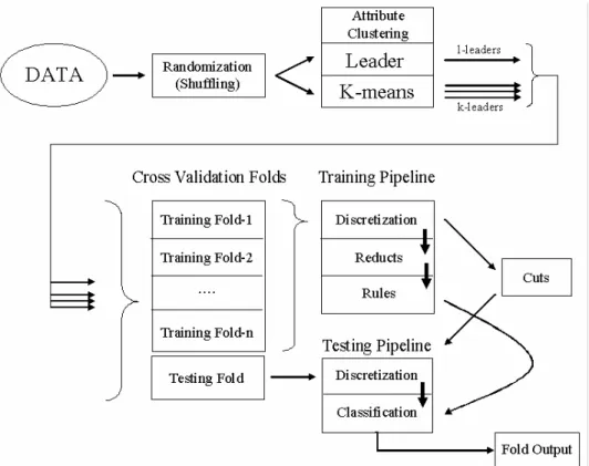
Rough sets analysis is combined with clustering, within a distributed (grid) computing environment for the analysis of microarray data in ([66], [67], [68]). Neural networks, genetic programming and virtual reality visualization techniques ([65]) are used at a post# processing stage. The strategy is to create an automated pipelined mining machine as illustrated in Fig. 3.
Fig. 3. Data processing strategy combining clustering with Rough Sets analysis and cross# validation.
In a first step, the objects in the dataset are shuffled using a randomized approach in order to reduce possible biases. Then, the attributes of the shuffled dataset
are clustered using two families of clustering algorithms: the leader (two variants), and k# means (four variants). For a given clustering solution, each of the formed clusters of attributes is represented by exactly one of the original data attributes (the l#leader or k# leader according to the family of clustering algorithm used). For the corresponding clustering scheme, their collection induces a new information system (subset of the original one) amenable to rough sets analysis which proceeds as a n#fold cross#validation
process in which for each training fold the following processing is applied: discretiztion (according to different techniques), reduct computation, rule
generation. Then the corresponding test fold is: discretized using the corresponding cut points found for the training fold and classified with the set of rules obtained for the training fold. In this way the generalization ability of the generated rules can be evaluated by looking at their min, max and average performance in the different cross#validation folds.
Cross#validation and bootstrapping are both methods for estimating generalization error based on "resampling" ([71]; [26]; [40]). The resulting estimates of generalization error are often used for choosing among various classification or regression models. In k#fold cross#validation, the data is divided into k subsets of approximately equal size. The model id trained k#times, each time leaving out one of the subsets from training, but using only the omitted subset to compute whatever error measure is used. If k equals the sample size, this is often called "leave#one#out" cross#validation. A more elaborate and expensive version of cross#validation is called "Leave#v#out" and involves leaving out all possible subsets of v cases.
Each processing stage feeds its results to the next, yielding a pipelined data analysis stream. The whole process is automated using the Condor high#throughput distributed
(grid) computing environment ([6]), ( with algorithms
from the ROSETTA system in batch processing mode embedded ([68]). In the first version ([66]), the RSES system for rough sets processing was used ([10]).
This approach has been applied to: the Leukemia gene expression dataset reported in [34], consisting of 72 samples from patients with acute lymphoblastic leukemia (ALL) and acute myeloid leukemia (AML), characterized by 7129 genes ([66], [67), and the Breast Cancer dataset described by [21], which consists of 24 core biopsies taken from patients found to be (greater than 25% residual tumor volume) or (less than 25% residual tumor volume) to docetaxel treatment, with 12,625 genes placed onto the microarray (Valdés and Barton 2006).
In the Leukemia application, two variants of leader clustering with 8 different similarity thresholds and 4 variants of k#means were used (Forgy, Jancey, Convergent and
MacQueen). Rough sets algorithms considered 4 discretization techniques (Boolean reasoning, Entropy, Naïve and Semi#Naïve) with two reduct computation algorithms (Johnson and Holte) on 10 cross#validation folds. In the best experiment, a mean classification accuracy of 0.925 was obtained. Also a set of relevant genes were identified, from which many coincided with those reported ([34], [28]).
Important research goal are to model the relationships between gene expression as a function of time, the involvement of a gene in a given biological process and the use of the model to predict the biological roles of unknown genes. Rough sets are used ([46]) to build rule models with minimal features as prediction attributes for Gene Ontology classes of biological processes. Temporal gene transcript profiles from 24 h fibroblast serum responses data ([42]) were used in the study. The rule#based classifiers were obtained with the ROSETTA system. Genetic algorithms were used to find approximate reducts (those that only preserve the discriminatory properties for a large fraction of the examples), as they may provide better classification rules and tend to avoid overtraining.
10#fold cross#validation over the training examples was used to assess the classification quality of the method and 84% of all annotations for the training examples could be classified correctly. A considerable number of the hypothesized new roles for known genes were confirmed by literature search. Moreover, many biological process roles hypothesized for uncharacterized genes were found to agree with assumptions based on additional information.
An important contribution from the point of view of understanding the development of metastatic adenocarcinoma (of unknown origin) and the development of better diagnostic markers is presented in [25]. In that study, expression profiling of 27 candidate markers was done using tissue microarrays and immunohistochemistry. In a first round, 352 primary adenocarcinomas from seven main sites (breast, colon, lung, ovary, pancreas, prostate and stomach) were considered, including their differential diagnoses. A
combination of rough sets methods (rules found with ROSETTA) and decision trees were used in order to construct a classification scheme. From the original 27 candidate
markers, 10 were found important and a classification rate of 88% was obtained using all of the original markers. The same rate was achieved on a test set of 100 primary and 30 metastases tumors using the 10 relevant markers derived from the data analysis process. These results enable better prediction on biopsy material of the primary cancer site in patients with metastatic adenocarcinoma of unknown origin, leading to improved management and therapy
.
Another rough sets based approach for microarray data is presented in [29], [30]. It is illustrated with the Leukemia data from [34] with cancer data reported by [48]. The
algorithm used is MLEM2, which is part of the LERS data mining system ([35], [36], [37]).
In the first step of processing, the input data is checked for consistency. If the input data is inconsistent, lower and upper approximations of all concepts are computed. Rules induced from the lower approximation of the concept certainly describe the concept and they are called . Rules induced from the upper approximation of the concept describe the concept only plausibly and they are called .
The algorithm learns the smallest set of minimal rules describing the concept by exploring the search space of attribute#value pairs. The input data is a lower or upper approximation of a concept, so the algorithm always works with consistent data. The algorithm computes a local covering and then converts it into a rule set. The main underlying concept is that of an attribute#value block, which is the set of objects sharing the same value for a given attribute.
A lower or upper approximation of a concept defined for the decision attribute is said to on a set of attribute#value pairs if and only if the intersection of all of its blocks is a subset of the given lower or upper approximation. A set of attribute#value pairs (T) is a
of a lower or upper approximation of a concept defined for the decision attribute (B), if and only if it depends on T and not on any of its proper subsets.
A collection of sets of attribute#value pairs is said to be a of B if and only if: each member the collection is a minimal complex of B can be formed by the union of all of the sets of the collection with minimal cardinality For a lower or upper approximation of a concept defined for the decision attribute, the LEM2 algorithm produces a single local covering. Its improved version (MLEM2) recognizes integer and
real numbers as values of attributes; computing blocks in a different way than for symbolic attributes.
It is interesting that no explicit discretization preprocessing is required due to the way in which blocks are computed for numeric attributes. It combines attribute#value pairs relevant to a concept and creates rules describing the concept. Also it handles missing attribute values during rule induction. Besides the induction of certain rules from
incomplete decision tables with missing attribute values interpreted as lost, MLEM2 can induce both certain and possible rules from a decision table with some missing attribute values. They can be of two kinds: “lost” and "do not care". Another interesting feature of this approach is a mining process based on inducing several rule generations.
The original rule set is the first generation rule set. Dominant attributes involved in the first rule generation are excluded from the data set. Then a second rule generation is induced, and so on. The induction of many rule generations is not always feasible, but for microarray data, where the number of attributes (genes) is very large compared to the number of cases, it is. In general, the first rule generation is more valuable than the second rule generation because it is based on a stronger set of condition attributes. Then the second rule generation is more valuable than the third and so on. Rule generations are gradually collected into new rule sets in a process that is repeated until no better sets are obtained in terms of error rates.
When applied to the Leukemia data from [34], it was found that the classifiers produced excellent performance. Moreover, many of the genes that were found are relevant to leukemia and coincide with genes found to be relevant in previous studies ([34], [28], [66]).
The approach was equally successful when applied to the microRNA cancer data ([48]). All but one case of breast cancer and all cases of ovary cancer were correctly classified using seven attributes (microRNAs), from which the functions of four have not yet been determined. For the remaining three with known functions, the connection with certain types of tumors has been clearly established.
- :
Many researchers consider the forthcoming decades as the based on their view that the technical problems for obtaining genomic information have been resolved. However, the understanding of the (all of the proteins in a cell at a given time) poses a big challenge. One main reason is the lack of suitable methods for defining proteomes, which is also related to the increased level of problem complexity. Whilst each of the cells of a given organism has the same DNA, the protein content of a cell depends on the cell type, for which there are many. Moreover, the proteome of a cell changes over time in response to fluctuations in the intra and extra cellular environments. According to the Central Dogma of Biology, a DNA sequence encodes the protein
sequence, which determines the 3D structure of the protein. On the other hand, it is known that protein 3D structure is related with its function. However, proteins are more difficult to analyze than DNA. For proteins there is no chemical process like the
polymerase reaction by means of which copies of DNA sequences can be made. Very sensitive and accurate techniques, like mass spectrometry, must be used in order to
analyze relatively small numbers of molecules which are produced , in
contradistinction with DNA. The information of the DNA (expressed in the four letter language of the nucleotide bases: adenine (A), thymine (T), guanine (G), and cytosine (C)), is converted into a protein which is a sequence of amino acids (20 of them can be used, thus determining a 20#letter alphabet), formed in a way somewhat similar to the nucleotide strand (DNA). Although DNA sequences contain all of the information that is translated into a protein sequence, the converse doesn’t hold because in DNA sequences there is information related to the control and regulation of protein expression which can not be extracted from the corresponding protein sequence. Unfortunately, the
computational methods available for determining which part of the DNA sequence is translated into a protein sequence and which parts have other possible roles can not provide complete accuracy. Actually, several years after the human genome has been released, there is no reliable estimate of the number of proteins that it encodes. This is a strong reason why known protein sequences should be studied.
Protein strands are much more flexible in space than DNA and form complex 3D structures.
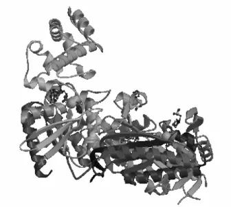
The individual amino acids compose a string which makes a protein and are called . In a process still not understood, the protein folds into a 3D structure (in fact sometimes other proteins help a particular protein fold; the so called ). It is considered that the particularities of this 3D structure determine the functions of the protein. The original chain of residues is called the of the protein. The resulting 3D structure (known as the of the protein) is composed by an arrangement of smaller local structures, known as . They are
composed of helices (α#helices, which are right#handed helical folds), strands (β#sheets, which are extended chains with conformations that allow interactions between closely folded parallel segments) and other non#regular regions (Fig. 4). The is the overall 3D structure of the protein, which involves combinations of secondary
structure elements in some specific macro#structured ways. Several cases are
distinguished: all#α: composed mostly of α#helices, all#β: composed mostly of β# Fig. 4. A visualization of a protein showing structural elements like helices and strands.
sheets, α/β: most regular and common domain structures consist of repeating β#α#β super#secondary units and α+β: there are significant alpha and beta elements mixed, but not exhibiting the regularity found in the α/β type.
Recently, the Human Proteome Initiative has been launched
(http://ca.expasy.org/sprot/hpi/). So far, , the study of the proteome, has been more difficult than genomics because the amount of information needed is much larger. It is necessary to find what is the molecular function of each protein, what are the biological processes in which a given protein is involved, and where in the cell the protein is
located. One specific problem is related to the 3D structure of a protein (structure prediction is one of the most important computational biology problems) and concerted efforts are systematically oriented towards the solution of this problem
(http://predictioncenter.org/casp7/). Another problem is protein identification, location and quantification. Individual proteins have a stochastic nature which needs to be understood in order to assess its effect on metabolic functions.
Proteomics is a rapidly growing field, especially now in the post#genomic era, with methods and approaches which are constantly changing. As with genomics, granular computing is finding its place within the set of computational techniques applied.
- # 7 88
:
Fuzzy sets have been applied to the problem of predicting protein structural classes from amino acid composition. Fuzzy c#means clustering ([14]) was used in a pioneering work by [77], for classifying globular proteins into the four structural classes (all#α, all#β, α/β and α+β) depending upon the type, amount and arrangement of secondary structures
present. Each of the structural classes is described by a fuzzy cluster and each protein is characterized by its membership degree to the four clusters and a given protein is classified as belonging to that structural class corresponding to the fuzzy cluster with maximum membership degree. A training set of 64 proteins was studied and the fuzzy # means algorithm was used for computing the membership degrees. Results obtained for the training set show that the fuzzy clustering approach produced results comparable to or better than those obtained by other methods. A test set of 27 proteins also produced comparable results to those obtained with the training set. This was an unsupervised approach using clustering to estimate the distribution of the training protein datasets. The prediction of the structural class of a given protein was based on a maximal membership function assignment, which is a simple approach.
From a supervised perspective, also using fuzzy methods, the same problem has been investigated in [59], using supervised fuzzy clustering ([1]). This is a fuzzy classifier which can be considered as an extension of the quadratic Bayes classifier that utilizes a mixture of models for estimating the class conditional densities. In this case, the overall success rate obtained by the supervised fuzzy #means (84.4 %) improved the one obtained with unsupervised fuzzy clustering by [77]. When applied to another dataset of 204 proteins ([23]), the success rates obtained with jackknifing also improved those obtained with classical fuzzy #means (73.5 % vs. 68.14 % and 87.25 vs. 69.12 % respectively).
Another direction pursued for predicting the 3D structure of a protein has been the prediction of solvent accessibility and secondary structure as an intermediate step. The reason is that a basic aspect of protein structural organization involves interaction of
amino acids with solvent molecules both during the folding process and in the final structure.
The problem of predicting protein solvent accessibility has been approached as a classification task using a wide variety of algorithms like neural networks, Bayesian statistics, SVMs, and others. In particular, a fuzzy #nearest neighbor technique ([16]) has been used for this problem ([61]), which is a simple variant of the classical “hard” # nearest neighbor classifier where the exponent of the distance between the feature vectors of the query data and its i#th nearest reference data is affected by a fuzzy strength parameter which determines how heavily the distance is weighted when calculating each neighbor’s contribution to the membership value, and the fuzzy membership of the reference vectors to the known classes is used as a weighting factor for the distances. With this approach, the ASTRAL SCOP dataset ([3]) was investigated. First, leave#one# out cross#validation on 3644 proteins was performed, where one of the 3644 chains was selected for predicting its solvent accessibility. The remaining 3643 chains were used as the reference dataset.
Although slight, the fuzzy #nearest neighbor method exhibited better prediction accuracies than other methods like neural networks and SVMs, which is remarkable, considering the simplicity of the #nearest neighbor family of classifiers in comparison with the higher degree of complexity of the other techniques.
Clearly, protein identification is a crucial task in proteomics where several techniques like 2D gel electrophoresis, amino acid analysis and mass spectrometry are used. 2#D gel electrophoresis is a method for the separation and identification of proteins in a sample by displacement in two dimensions oriented at right angles to one another. This
allows the sample to separate over a larger area, increasing the resolution of each component and is a multistep procedure that can separate hundreds to thousands of proteins with high resolution. It works by separating proteins by their
(which is the pH at which a molecule carries no net electrical charge) in one dimension, and by their molecular weight in the second dimension.
Examples of 2D gels from the GelBank database ([33]) are shown in Fig. 5, where both the blurry nature of the spots corresponding to protein locations and the deformation effects due to instrumental and other experimental conditions can be observed.
Fig. 5. GelBank images of 2D gels ( ). The horizontal axis is the isoelectric point and the vertical axis is the molecular weight. Left: S#oneidensis (aerobic
growth). Right: P#furiosus (cells grown in the absence of sulfur). Observe the local deformations of the right hand side image.
2D gel electrophoresis is generally used as a component of proteomics and is the step used for the isolation of proteins for further characterisation by mass spectroscopy. Another use of this technique is , where the purpose is to compare two or more samples to find differences in their protein expression. For example, in a study looking at drug resistence, a resistent organism is compared to a susceptible one in an attempt to find changes in the proteins expressed in the two samples. 2#D gel
electrophoresis is a multistep procedure: the resulting gel is stained for viewing the protein spots, it is scanned resulting in an image and mathematical and computer procedures are applied in order to perform comparison and analysis of replicates of gels. The objective is to determine statistically and biologically meaningful spots.
The uncertainty of protein location in 2D gels, the blurry character of the spots and the low reproducibility of this technique make the use of fuzzy methods very appealing. A fuzzy characterization of spots in 2D gels is described in [49]. In this approach the theoretical crisp protein location (a point) is replaced by a spot characterization via a two dimensional Gaussian distribution function with independent variances along the two axis. Then, the entire 2D gel is modeled as the sum of the set of Gaussian functions contained and evaluated for the individual cells in which the 2D gel image was digitized. These fuzzy matrices are used as the first step in a processing procedure for comparing 2D gels based on the computation of a similarity index between different matrices. This similarity is defined as a ratio between two overall sums over all of the cells of the two 2D gels compared: the one corresponding to the pairwise minimum fuzzy matrix elements and that of the pairwise maximum fuzzy matrix values ([50]). Then, multiple 2D gels are compared by analyzing their similarity matrices by a suite of multivariate
methods like clustering, MDS and others. The application of the method to a complex dataset constituted by several 2#D maps of sera from rats treated with nicotine (ill) and controls has shown that this method allows discrimination between the two classes. Another crucial problem associated with 2D gel electrophoresis is the automated comparison of two or more gel images simultaneously. There are many methods for the analysis of 2D gel images but most of the available techniques require intensive user interactions, which creates a major bottleneck and prevents the high throughput
capabilities required to study protein expression in healthy and diseased tissues, where many samples ought to be compared.
An automatic procedure for comparison of the 2D gel images based on fuzzy methods, in combination with global or local geometric transform and brightness interpolation on the images was developed in [44], [45]. The method uses an iterative algorithm, alternating between correspondence and spatial global mapping. The features (spots) are described by Gaussian functions with σ as a fuzziness parameter and the correspondence between two images is represented by a matrix with the rows and columns summing to unit, where its cells measure the matching between the #th spot on image A with the #th spot on image B. These elements are then used as weights in the feature transform. In the process, a starting a fuzziness parameter σ is chosen, which is decreased progressively until
convergence in the correspondence matrix is obtained. Fuzzy matching is performed for spot coordinates, area and intensity at the maximum, i.e., each spot is described by four parameters, however, spot coordinates are considered as two times more important than the area and intensity. The spatial mapping is performed by bilinear transforms of one image onto the other composed of the inverse and forward transforms. When
characterizing the overall geometric distortion between the images one single mapping function can be considered (global transform). However, to deal with local distortions of 2D gel images, piecewise transformations can be used, in this case based on Delaunay triangulation for tessellating the images with linear or cubic interpolation within the resulting triangles. Image brightness is also interpolated and pseudo#color techniques are used for the visualization of matched images.
This method of gel image matching allows efficient automated matching of 2D gel electrophoresis images. Its efficiency is limited by the performance of fuzzy alignment used to align the sets of the extracted spots. Good results are also obtained with locally distorted 2D gels and the best results are obtained for linear interpolation of the grid and for cubic interpolation of the brightness.
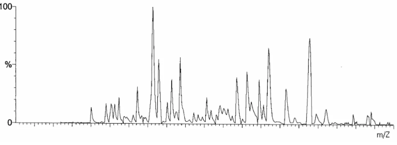
Mass spectrometry is a powerful analytical technique that measures the mass#to#charge ratio (m/z) of ions that is used to identify unknown compounds, to quantify known compounds, and to elucidate the structure and chemical properties of molecules, in particular, proteins (Fig. 6). Two of the most commonly used methods for quantitative proteomics are 2D electrophoresis coupled to either mass spectrometry (MS) or tandem mass spectrometry (MS/MS) and liquid chromatography coupled to mass spectrometry (LCMS).
With the advances in scientific instrumentation, modern mass spectrometers are capable of delivering mass spectra of many samples very quickly. As a consequence of this high rate of data acquisition, the rate at which protein databases are growing is also high and therefore high#throughput methods for the identification of peptide fragmentation spectra is becoming increasingly important. But typical analyses of experimental data sets obtained by mass spectrometry on a single processor takes on the order of half a day of computation time (for example, 30 000 scans against the Escherichia coli database). In addition, the search hits are only meaningful when ranked by a relatively computationally intensive statistical significance/relevance score. If modified copies of each mass
spectrum are added to the database in order to account for small peak shifts intrinsic to mass spectra owing to measurement and calibration error of the mass spectrometer,
Fig. 6. Mass spectrum from a sample of mouse brain tissue. The horizontal axis is the mass/charge ratio and the vertical axis is the relative intensity. The individual peaks correspond to different peptides present in the sample, according to their mass/charge
combinatorial explosion occurs because of the need of considering the more than 200 known protein modifications.
A ‘coarse filtering#fine ranking’ scheme for protein identification using fuzzy techniques as a fundamental component of the procedure has been introduced recently ([55]). It consists of a coarse filter which is a fast computation scheme that produces a candidate set with many false positives, without eliminating any true positives. The computation is often a lower bound with respect to more accurate matching functions, and it is less computationally intensive. The coarse filtering
stage improves on the shared peaks count, followed by a fine filtering stage in which the candidate spectra output by the coarse filter are ranked by a Bayesian scoring scheme. Mass spectra are represented as high dimensional vectors of mass/charge values; for convenience, transformed into Boolean vectors. For typical mass ranges, these vectors are ~50,000#dimensional. Therefore, the similarity measure used is a determining factor of the computational expense of the search. Typically, distance measures for comparison of mass spectra are used and since the specific locations of mass spectra peaks have an associated uncertainty, fuzzy measures are very appropriate. Given two Boolean vectors and a peak mass tolerance (a fuzziness parameter) measured in terms of the mass
resolution of the spectra analyzed, a tally measure between two individual mass spectrometry intensities for a given mass/charge ratio is defined. According to this measure, two peaks count as equal (a match) if they lie within a range of vector elements of each other, as determined by the peak mass tolerance. Then a
measure is defined as the ratio between the overall sum of the pairwise match measures and the product of the modules of the two Boolean vectors representing the spectra. This
similarity is transformed into a dissimilarity by taking its inverse cosine function, called the , which may fail to fulfill the identity and the triangular
inequality axioms of a distance in a metric space.
The precursor mass is the mass of the parent peptide (protein sub#chains). Another dissimilarity called the is defined as the difference in the precursor masses of two peptide sequences, semi#thresholded by a precursor mass tolerance factor, which acts as another fuzzification parameter. The idea is that if the absolute precursor mass difference is smaller than the tolerance factor, the precursor mass distance is defined as zero. Otherwise it is set to the absolute precursor mass difference. This measure is also a semi#metric, and the linear combination of the fuzzy cosine distance with the precursor mass distance is the so#called , carrying the idea of fuzziness in the comparison of the two mass spectra.
This is the measure used by the coarse filter function when querying the mass spectra database. With this ‘coarse filtering#fine ranking’ metric space indexing approach for protein mass spectra database searches, fast, lossless metric space indexing of high dimensional mass spectra vectors is achieved. The fuzzy coarse filter speeds up searches by reducing both the number of distance computations in the index search and the number of candidate spectra input to a fine filtering stage. Moreover, the measures represent biologically meaningful and computationally efficient distance measures. In fact the number of distance computations is less than 0.5% of the database and the number of candidates for fine filtering to approximately 0.02% of the database.
The prediction of the protein structure class (all#α, all#β, α/β and α+β) is one of the most important problems in modern proteomics and it has been approached using a wide variety of techniques like discriminant analysis, neural networks, Bayes decision rules, SVMs, boost of weak classifiers and others. Recently, rough sets have been applied as well ([19]). In the study, two datasets of protein domain sequences from the SCOP
database were used: one consisting of 277 sequences, and another with 498 sequences. In both cases, the condition attribute set was assembled with compositional percentages of the 20 amino acids in primary sequences and 8 physicochemical properties, for a total of 28 attributes. The decision attribute was the protein structure class consisting of the four previously mentioned categories. The ROSETTA system was used for rough sets
processing with semi#näive discretization and genetic algorithms for reduct computation. Self#consistency and jackknife tests were applied and the rough sets results were
compared with other classifiers like neural networks and SVMs. From this point of view, the performance of the rough set approach was on the average equivalent to that of SVM and superior to that of neural networks. For example, for the α/β class, the results
obtained with rough sets were the overall best with respect to the other algorithms (93.8 % for the first dataset composed of 277 sequences and 97.1 % for the second composed of 498). It was also proved that amino acid composition and physicochemical properties can be used to discriminate protein sequences from different structural classes, suggesting that a rough sets approach may be extended to the prediction of other protein attributes, such as sub#cellular location, membrane protein type and enzyme family classification. Proteomic biomarker identification is another important problem because in the search for early diagnosis in diseases like cancer, it is essential to determine molecular
parameters (so#called biomarkers) associated with the presence and severity of specific disease states. Rough sets have been applied to this problem ([17]) for feature selection in combination with blind source separation ([20]) in a study oriented to the identification of proteomic biomarkers of ovarian and prostate cancer. The information used was serum protein profiles as obtained by mass spectrometry in a dataset composed of 19 protein profiles belonging to two classes: myeloma (a form of cancer) and normal. Each profile was initially described by 30,000 values of mass to charge ratio (the attributes), as obtained from the mass spectrometer. Then, they were reduced to a subsequence of 100 by choosing those with the highest Fisher discriminant power. Blind source separation separated the subsequence into 5 source signals, further reduced to only two when reducts were computed. In order to verify the effect of the use of a reduced set of attributes in the classification, a neural network consisting of a single neuron was used. Average testing errors revealed that there was a generalization improvement with the use of a smaller number of selected attributes. Despite being in its early stages and hindered by the problem of determining the optimal number of sources to extract, this approach showed the advantages of combining rough sets with signal processing techniques.
Drug design is another important problem and the development of the so calledG# protein#coupled receptors (GPCRs) are among the most important targets. Their 3D structure is very difficult to find experimentally. Hence, computational methods for drug design have relied primarily on techniques such as 2D substructure similarity searching and quantitative structure activity relationship modeling ([4]). Very recently this problem has been approached from a rough sets perspective ([64]).
A ligand is a molecule that interacts with a protein, by specifically binding to the protein via a noncovalent bond while a receptor is a protein that binds to the ligand. Protein# ligand binding has an important role in the function of living organisms and is one method that the cell uses to interact with a wide variety of molecules.The modeling of the receptor#ligand interaction space is made using descriptors of both receptors and ligands. These descriptors are combined and associated with experimentally measured binding affinity data. From them, associations between receptor#ligand properties can be derived. In all of the three datasets investigated the condition attributes were descriptors of receptors and ligands and the decision attribute was a two category class of binding affinity values (low and high). The goal was to induce models separating high and low binding receptor#ligand complexes formulated as a set of decision rules obtained using the ROSETTA system. Three datasets were studied, and each was randomly divided into a training set of 80% (with 32, 48, 105 objects respectively) and an external test set composed of 20% of the objects (with 8, 12 and 26 objects respectively). The number of condition attributes for the three datasets was 6, 8 and 55 respectively.
Object related reducts were computed using Johnson’s algorithm ([43]) and rules were constructed from them. They were used for validation and interpretation of the induced models. Approximate reducts were computed by the genetic algorithms for an implicit ranking of attributes. Mean accuracy and area under the ROC curve (Receiver Operating Characteristic) served as measures of the discriminatory power of the classifiers
evaluated by cross#validation. The rough set models provided good accuracies in the training set, with mean 10#fold cross#validation accuracy values in the 0.81#0.87 range for the three datasets, and in the 0.88#0.92 range for the independent test set. These
results complement those obtained for the same datasets using the Partial Least Squares technique ([54]) for the analysis of ligand#receptor interactions. Besides quality and robustness, rough sets models have advantages like their minimality with respect to the number of attributes involved and their interpretability. All of them are very important because they provide a deeper understanding of ligand#receptor interactions.
Rough sets models have been proven to be successful and robust in, for example, fold recognition, prediction of gene function from time series expression profiles and the discovery of combinatorial elements in gene regulation. From the point of view of rough sets software tools used in bioinformatics, ROSETTA ([52]) is the one which has been mostly used, followed by RSES ([10]) and LERS ([35], [36]). It is important to observe that the effectiveness of rough set approaches increases when usedin combination with other computational intelligence techniques like neural networks, evolutionary
computation, support vector machines, statistical methods, etc.
;
All of these examples indicate that Granular Computing methods have a large potential in bioinformatics. Their capabilities for uncertainty handling, feature selection,
unsupervised and supervised classification and their robustness, among others, make them very powerful tools, useful for the problems of interest to both classical and modern bioinformatics. So far, fuzzy and rough sets methods have been the preferred granular computing techniques used in bioinformatics and they have been applied either alone or in combination with other mathematical procedures. Most likely this is the best strategy.
The number of applications in this domain is growing rapidly and this trend should continue in the future.
[1] J. Abonyi , F. Szeifert, Supervised Fuzzy Clustering for the Identification of Fuzzy Classifiers, Pattern Recognition Letters
[2] U. Alon, N. Barkai, D.A. Notterman, K. Gish, S. Ybarra, D. Mack, A.J. Levine , Broad patterns of gene expression revealed by clustering analysis of tumor and normal colon tissues probed by oligonucleotide arrays, Proc. Nat. Acad. Sci. USA, 96, 67, (1999) 45#6750.
[3] ASTRAL SCOP: The ASTRAL Compendium for Sequence and Structure Analysis, http://astral.berkeley.edu.
[4] J. Bajorath, Integration of virtual and high#throughput screening. Nat. Rev. Drug Discovery, 1, (2002) , 882–894.
[5] P. Baldi, S. Brunak, Bioinformatics: The Machine Learning Approach, MIT Press, 1999.
[6] J. Basney, M. Livny, T. Tannenbaum, High Throughput Computing with Condor. !"# $ , 1, 2, (1997).
[7] A..D. Baxevanis, B.F. Ouellette, Bioinformatics. A Practical Guide to the Analysis of Genes and Proteins, John Wiley, Hoboken, N.J., 2005
[8] J.G. Bazan, Dynamic reducts and statistical inference. Proc. Sixth Int. Conf. of Information Processing and Management of Uncertainty in Knowledge#Bases Systems (IPMU’96), 3, 1996.
[9] J. Bazan, H.S. Nguyen, S. N. Nguyen, P. Synak, , J. Wróblewski, Rough Set Algorithms in Classification Problem, In Rough Set Methods and Applications: new
developments in knowledge discovery in information systems, Physica#Verlag, (2000), 49#88.
[10] J.G. Bazan, S. Szczuka, J. Wróblewski, A New Version of Rough Set Exploration System, Third. Int. Conf. on Rough Sets and Current Trends in Computing RSCTC 2002, Malvern, PA, USA, Oct 14#17. Lecture Notes in Computer Science (Lecture Notes in Artificial Intelligence Series) LNCS 2475, Springer#Verlag, 2002, pp 397#404.
[11] N. Belacel, P. Hansen, N. Mladenovic, Fuzzy J#Means: A New Heuristic for Fuzzy Clustering, Pattern Recognition., 35 (2002), 2193–2200.
[12] N. Belacel, M. Čuperlović#Culf, M. Laflamme, R. Ouellette, Fuzzy J#Means and VNS Methods for Clustering Genes from Microarray Data, Bioinformatics 20 (2004), 1690#1701.
[13] J.C. Bezdek, Fuzzy Mathematics in Pattern Classification, Cornell University, 1973.
[14] J.C. Bezdek, Pattern Recognition with Fuzzy Objective Function, Plenum Press, 1981.
[15] J.C. Bezdek, S.K. Pal, Fuzzy models for pattern recognition method that search for structures in data. IEEE press, 1992.
[16] J.C. Bezdek, L.O. Hall, L.P. Clark, Review of MR image segmentation techniques using pattern recognition, % ! , 20, (1993) 1033–1048.
[17] G.M. Boratyn, T.G. Smolinski, J.M. Zurada, M. Mariofanna Milanova, S.
Bhattacharyya, L.J. Suva, Hybridization of Blind Source Separation and Rough Sets for Proteomic Biomarker Identification, Proc. ICAISC 2004, (Lecture Notes in Artificial Intelligence Series) LNAI 3070, 2004, pp. 486–491.