HAL Id: hal-01207395
https://hal.sorbonne-universite.fr/hal-01207395
Submitted on 30 Sep 2015
HAL is a multi-disciplinary open access
archive for the deposit and dissemination of
sci-entific research documents, whether they are
pub-lished or not. The documents may come from
teaching and research institutions in France or
abroad, or from public or private research centers.
L’archive ouverte pluridisciplinaire HAL, est
destinée au dépôt et à la diffusion de documents
scientifiques de niveau recherche, publiés ou non,
émanant des établissements d’enseignement et de
recherche français ou étrangers, des laboratoires
publics ou privés.
and zooplankton fecal pellets to carbon export: insights
from free-drifting sediment trap deployments in
naturally iron-fertilised waters near the Kerguelen
Plateau
E. C. Laurenceau-Cornec, T. W. Trull, D. M. Davies, S. G. Bray, J. Doran,
Frédéric Planchon, F Carlotti, M.-P. Jouandet, A.-J. Cavagna, A. M. Waite,
et al.
To cite this version:
E. C. Laurenceau-Cornec, T. W. Trull, D. M. Davies, S. G. Bray, J. Doran, et al.. The relative
importance of phytoplankton aggregates and zooplankton fecal pellets to carbon export: insights from
free-drifting sediment trap deployments in naturally iron-fertilised waters near the Kerguelen Plateau.
Biogeosciences, European Geosciences Union, 2015, 12 (4), pp.1007-1027. �10.5194/bg-12-1007-2015�.
�hal-01207395�
www.biogeosciences.net/12/1007/2015/ doi:10.5194/bg-12-1007-2015
© Author(s) 2015. CC Attribution 3.0 License.
The relative importance of phytoplankton aggregates and
zooplankton fecal pellets to carbon export: insights from
free-drifting sediment trap deployments in naturally iron-fertilised
waters near the Kerguelen Plateau
E. C. Laurenceau-Cornec1,2, T. W. Trull2,3, D. M. Davies2, S. G. Bray2, J. Doran4, F. Planchon5, F. Carlotti6, M.-P. Jouandet6, A.-J. Cavagna7, A. M. Waite4,8, and S. Blain9,10
1CSIRO-UTAS Quantitative Marine Sciences PhD Program, Institute for Marine and Antarctic Studies,
University of Tasmania, Private Bag 129, Hobart TAS 7001, Australia
2Antarctic Climate and Ecosystems Cooperative Research Centre, University of Tasmania, Private Bag 80, Hobart TAS 7001,
Australia
3Commonwealth Scientific and Industrial Research Organisation, Marine and Atmospheric Research, Castray Esplanade,
Hobart TAS 7000, Australia
4UWA Oceans Institute, The University of Western Australia (M470), 35 Stirling Highway, Crawley WA 6009, Australia 5Laboratoire des Sciences de l’Environnement Marin (LEMAR), Université de Brest, CNRS, IRD, UMR6539, IUEM,
Technopôle Brest Iroise, Place Nicolas Copernic, 29280 Plouzané, France
6Mediterranean Institute of Oceanography (MIO), Aix-Marseille Université, CNRS-IRD, 13288 Marseille, CEDEX 09,
France
7Vrije Universiteit Brussel, Analytical and Environmental Geochemistry Dept., Brussels, Belgium
8Alfred Wegener Institute Helmholz Centre for Polar and Marine Research, Building E-2155, Am Handelshafen 12,
27570 Bremerhaven, Germany
9Sorbonne Universités, UPMC Univ. Paris 06, UMR 7621, Laboratoire d’Océanographie Microbienne,
Observatoire Océanologique, 66650 Banyuls/mer, France
10CNRS, UMR 7621, Laboratoire d’Océanographie Microbienne, Observatoire Océanologique, 66650 Banyuls/mer, France
Correspondence to: E. C. Laurenceau-Cornec (emmanuel.laurenceau@utas.edu.au)
Received: 18 August 2014 – Published in Biogeosciences Discuss.: 19 September 2014 Revised: 16 December 2014 – Accepted: 5 January 2015 – Published: 17 February 2015
Abstract. The first KErguelen Ocean and Plateau compared Study (KEOPS1), conducted in the naturally iron-fertilised Kerguelen bloom, demonstrated that fecal material was the main pathway for exporting carbon to the deep ocean during summer (January–February 2005), suggesting a limited role of direct export via phytodetrital aggregates. The KEOPS2 project reinvestigated this issue during the spring bloom ini-tiation (October–November 2011), when zooplankton com-munities may exert limited grazing pressure, and further ex-plored the link between carbon flux, export efficiency and dominant sinking particles depending upon surface plank-ton community structure. Sinking particles were collected in polyacrylamide gel-filled and standard free-drifting
sed-iment traps (PPS3/3), deployed at six stations between 100 and 400 m, to examine flux composition, particle origin and their size distributions. Results revealed an important contri-bution of phytodetrital aggregates (49 ± 10 and 45 ± 22 % of the total number and volume of particles respectively, all sta-tions and depths averaged). This high contribution dropped when converted to carbon content (30 ± 16 % of total carbon, all stations and depths averaged), with cylindrical fecal pel-lets then representing the dominant fraction (56 ± 19 %).
At 100 and 200 m depth, iron- and biomass-enriched sites exhibited the highest carbon fluxes (maxima of 180 and 84 ± 27 mg C m−2d−1, based on gel and PPS3/3 trap collection respectively), especially where large fecal pellets dominated
over phytodetrital aggregates. Below these depths, carbon fluxes decreased (48±21 % decrease on average between 200 and 400 m), and mixed aggregates composed of phytodetri-tus and fecal matter dominated, suggesting an important role played by physical aggregation in deep carbon export.
Export efficiencies determined from gels, PPS3/3 traps and234Th disequilibria (200 m carbon flux/net primary pro-ductivity) were negatively correlated to net primary produc-tivity with observed decreases from ∼ 0.2 at low-iron sites to ∼ 0.02 at high-iron sites. Varying phytoplankton commu-nities and grazing pressure appear to explain this negative relationship. Our work emphasises the need to consider de-tailed plankton communities to accurately identify the con-trols on carbon export efficiency, which appear to include small spatio-temporal variations in ecosystem structure.
1 Introduction
Physical and biological processes occurring in the surface ocean generate a vast diversity of particles. These particles represent potential vehicles to export organic carbon to the deep ocean, where a small fraction can eventually be se-questered in the sediments. This process, known as the “bi-ological carbon pump” (BCP), influences the level of atmo-spheric carbon dioxide and thus the global climate system (Volk and Hoffert, 1985; Lam et al., 2011).
Primary production in the euphotic layer builds a stock of phytoplankton cells. If their concentration and stickiness are high enough (Jackson, 1990), these cells can collide, at-tach and form large phytodetrital aggregates (Burd and Jack-son, 2009; McCave, 1984), with those reaching sizes greater than 0.5 mm known as “marine snow” (Alldredge and Sil-ver, 1988). Alternatively, phytoplankton cells can be tightly packed into dense fecal pellets through zooplankton grazing (Silver and Gowing, 1991). Because of their large size and high density respectively, phytodetrital aggregates and fe-cal pellets are major constituents of the downward flux, and several studies have found either fecal pellets (Fowler and Knauer, 1986; Pilskaln and Honjo, 1987; Bishop et al., 1977; Wassmann et al., 2000; Ebersbach and Trull, 2008; Cavagna et al., 2013) or large organic aggregates (Turner, 2002; All-dredge and Gotschalk, 1989; De La Rocha and Passow, 2007; Jackson, 1990; Burd and Jackson, 2009) to be the dominant vectors of carbon to depth.
Because grazing causes losses of organic carbon by res-piration (Michaels and Silver, 1988; Alldredge and Jackson, 1995), direct export via the sinking of phytodetrital aggre-gates represents the most efficient operating mode of the BCP. However, the ecosystem structure and environmental conditions under which primary production can be exported directly via phytodetrital aggregates are still unclear, and their determination would considerably improve the predic-tions of the efficiency of the BCP in varying condipredic-tions.
The volume fraction of phytodetrital aggregates vs. fecal pellets in the total flux and their volume-to-carbon-content ratio select the dominant carbon export mode; these rela-tive contributions depend on numerous parameters, including primary productivity, biomass, interactions between primary producers and heterotrophic communities (Michaels and Sil-ver, 1988), physical fragmentation, microbial decomposition, coprophagy and the velocity at which particles settle (Turner, 2002).
The Southern Ocean contains the largest high-nutrient, low-chlorophyll (HNLC) area of the world ocean and is an essential player in global biogeochemistry (Sigman and Boyle, 2000). In these waters, abundant macronutrients (sili-cic acid, nitrate and phosphate) can fuel primary produc-tion given available light and sufficient iron, a limiting mi-cronutrient (de Baar et al., 1995; Martin, 1990). The Ker-guelen Plateau offers the opportunity to study the function-ing of the BCP in a naturally iron-fertilised region (Blain et al., 2007). The first KErguelen Ocean and Plateau com-pared Study (KEOPS1), demonstrated that most of the sink-ing flux collected in polyacrylamide gel sediment traps was derived from copepod fecal detritus (intact or degrading pel-lets and fecal material reaggregated with phytodetritus, here-after called “fecal aggregates”), and reported limited evi-dence for phytodetrital aggregates formed by direct floccu-lation of phytoplankton cells (Ebersbach and Trull, 2008). Number and volume fluxes were dominated by aggregates but represented a small fraction of the total carbon flux, ow-ing to their low volume-to-carbon-content ratio. Several nat-ural and artificial iron-fertilisation experiments conducted at the same time of the year but in different locations in the Southern Ocean (e.g. SAZ-Sense study and SOFeX) dis-played similar export modes relying mainly on fecal mat-ter (Bowie et al., 2011; Ebersbach et al., 2011; Coale et al., 2004; Lam and Bishop, 2007). In contrast, other artifi-cial and natural iron experiments (SOIREE, CROZEX and EiFeX) have demonstrated a direct export via the sinking of phytodetrital aggregates or single phytoplankton cells (Boyd et al., 2000; Waite and Nodder, 2001; Pollard et al., 2007; Salter et al., 2007; Smetacek et al., 2012).
These variations among studies may reflect the time-varying aspects of export. In his review of Southern Ocean ecosystem contribution to carbon export, Quéguiner (2013) suggests that from the onset of a bloom to its decline and subsequent export event, phytoplankton, and to a lesser ex-tent zooplankton communities, is subject to several rapid suc-cessions. The complexity of the processes is also reflected by the past 30 years of empirical and modelling studies attempt-ing to relate deep carbon export variations to surface produc-tivity (Eppley and Peterson, 1979; Suess, 1980; Wassmann, 1990; Guidi et al., 2009). In general, the ratio between ex-port and production in the surface ocean is low (< 5–10 %; Buesseler, 1998), but decoupling associated with high-export events (e.g. high-latitude blooms), or even negative relation-ships, has been noted (Maiti et al., 2013; Buesseler, 1998;
Ebersbach et al., 2011; Lam and Bishop, 2007). This high-lights the complexity of food web structure and its multiple controls on carbon export (Wassmann, 1998; Michaels and Silver, 1988).
In the present study we test the hypothesis that direct export via phytodetrital aggregates occurs during the early stage of the Kerguelen naturally iron-fertilised bloom, when zooplankton communities present in the water column are not fully developed. We further explore the relative export abilities of each carbon export mode (i.e. phytodetrital ag-gregates vs. fecal pellets) by looking at their variation with depth and over time and their links to spatio-temporal varia-tions in plankton communities.
We collected sinking particles in free-drifting polyacry-lamide gel and standard sediment traps. Gel traps allowed for the collection of intact natural particles as they sank in the water column (Ebersbach and Trull, 2008; Jannasch et al., 1980; McDonnell and Buesseler, 2010), and thus gave a direct “picture” of the sinking flux at the depth of trap de-ployment. Image analysis of particles embedded in gels pro-vided particle statistics (e.g. number and volume fraction of each category of particle), and conversion from area to vol-ume and from volvol-ume to carbon content, using empirical re-lationships, allowed for estimation of the carbon flux and the relative importance of each category of particle. In parallel, standard sediment traps serving as a reference permitted di-rect quantitative estimates based on bulk chemical analyses of the material collected and from234Th depletion method (Planchon et al., 2014). Then, to test our main hypothesis, the relative contribution of each category of particles was linked to the amount of carbon effectively exported in order to de-termine which one led the carbon export.
2 Material and methods
2.1 The KEOPS2 study
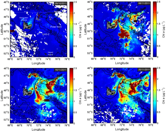
The second KErguelen Ocean and Plateau compared Study (KEOPS2) was conducted onboard the RV Marion Dufresne over and downstream of the Kerguelen Plateau, from 8 Oc-tober to 30 November 2011. Sinking particle flux and com-position were assessed by the use of free-drifting sediment traps deployed at six stations, inside and outside the natu-rally iron-fertilised area, in waters with varying biomass and surface chlorophyll a (Chl a) levels (Figs. 1 and 2). For more information on the complex spatio-temporal evolution of the phytoplankton bloom over the full 2011–2012 annual cycle, we refer the reader to an animation of NASA MODIS Aqua chlorophyll images, provided as a supplementary material in Trull et al. (2014). Combination of sediment trap collection with volume-to-carbon conversion factors allowed to deter-mine preferential modes of carbon export (Ebersbach and Trull, 2008; Ebersbach et al., 2011).
2.2 Water column properties and biomass at each station
In addition to trap-derived measurements, POC concentra-tions were estimated in the water column using a WET Labs C-Star (6000 m) transmissometer (660 nm wavelength and 25 cm path length) linked to a conductivity–temperature– depth (CTD) system (Sea-Bird SBE-911+CTD). Xmiss transmissometer data (%) were converted to POC concen-trations (µmol L−1) following a calibration based on in situ POC measurements from Niskin bottles. A Seapoint Chelsea Aquatracka III (6000 m) chlorophyll fluorometer linked to the CTD was used to determine fluorescence profiles. Flu-orescence was converted to chlorophyll a (Chl a; µg L−1)
by comparison with total Chl a in situ measurements from Niskin bottles (Lasbleiz et al., 2014).
Figure 2 shows water column properties and biomass at each site. The HNLC reference station R-2 located outside the fertilised area was characterised by a rela-tively deep mixed layer (96 m), low net primary produc-tivity (NPP) (euphotic zone 1 % PAR-integrated NPP = 135 ± 6 mg C m−2d−1; Cavagna et al., 2014), low sur-face chlorophyll (chlorophyll a mixed layer average = 0.6 µg Chl a L−1), and biomass (mixed-layer-integrated POC = 4.7 g C m−2). Stations E-1, E-3 and E-5 were located in an eddy-like, bathymetrically trapped recirculation feature in deep waters east of the Kerguelen Islands (stationary me-ander of the polar front), with a mixed layer depth varying from 33 (E-3) to 70 m (E-1). These stations had moderate NPP (523±55, 686±97 and 943±113 mg C m−2d−1
respec-tively), Chl a (0.8, 0.7 and 1.1 µg Chl a L−1 respectively), and biomass (5.3, 3 and 4.8 g C m−2respectively). They were used as a time series assuming a pseudo-Lagrangian evo-lution (d’Ovidio et al., 2014). F-L was the only station lo-cated north of the polar front and exhibited the shallowest mixed layer (31 m). A3-2 was the second visit to the on-plateau bloom reference station of KEOPS1 and had the deepest mixed layer (149 m). F-L and A3-2 displayed the highest NPP (3.4 ± 0.1 and 1.9 ± 0.2 g C m−2d−1 respec-tively), chlorophyll a (3 and 1.8 µg Chl a L−1respectively) and biomass (6.2 and 20.4 g C m−2).
2.3 Sediment trap preparation, deployments and recovery
Two different types of trap were deployed during KEOPS2. Bulk fluxes of particulate organic carbon (POC), total par-ticulate nitrogen (TPN), biogenic silica (BSi), parpar-ticulate in-organic carbon (PIC), particulate iron (PFe; data shown in Bowie et al., 2014) and thorium 234 (234Th) were estimated using PPS3/3 traps (Technicap, La Turbie, France). A PPS3/3 trap consists of a single cylindrical trap with an internal con-ical funnel at its base with a collection area of 0.125 m2 that transfers samples into a carousel of 12 cups. During KEOPS2, these traps were deployed for a maximum period
A3-2 F-L N 1 3 5 R-2 E Kerguelen islands Heard island Polar front 28/10/2011 06/11/2011 20/11/2011 16/11/2011 A3-2 F-L 1 3 5 R-2 E A3-2 F-L 1 3 5 R-2 E F-L 1 3 5 R-2 E A3-2
Figure 1. MODIS-Aqua satellite (CLS-CNES) images of surface chlorophyll a concentration (Chl a) at different bloom stages from 28
Oc-tober to 20 November 2011. Images show free-drifting sediment trap deployment locations in contrasting biomass levels. On each map, red labels represent the station(s) sampled at the date of the map ±3 days.
of 6 days. Cups were filled with brine with a salinity of ∼ 52 psu, made by freezing filtered (0.2 µm pore size) surface seawater. Some cups were also amended with mercuric chlo-ride (1 g L−1) as a biocide (as detailed in Table 4). No poison was added to the cups used for trace metal studies (Bowie et al., 2014).
To examine sinking flux characteristics (particle type, number and size), intact particles were also collected in cylindrical polyacrylamide gel-filled sediment traps with a collection area of 0.011 m2. These deployments lasted less than 2 days so as not to overload the gels (Table 1). Polyacry-lamide gels were prepared following the method developed by Lundsgaard (1995), modified as described in Ebersbach and Trull (2008).
Due to different required deployment durations (shorter for gel traps to avoid overloading; see above), each cate-gory of trap was deployed on separate arrays, except at A3-2 (combined deployment, Table 1). All separated deploy-ments of gel and PPS3/3 traps overlapped in time and
lo-cation (except at station E-3, where they were successive), to optimise the collection of similar particle fields. The ar-rays had broadly the same design consisting of a surface float sustaining a mooring line where the traps were fixed at different depths. PPS3/3 traps were fixed at 210 m, and one to four gel traps, depending on the station, were fixed at 110, 210, 330 and 430 m. Wave-induced motions were dampened by an elastic link to keep the traps at a constant depth (Trull et al., 2008). Pressure sensors mounted on the deepest gel trap and PPS3/3 trap on most of the arrays con-firmed very small vertical motions during the deployments, with depth standard deviations ranging from 0.6 m at E-1 to 2.4 m at E-5 (Table 1). The average trap drift speed of 8.5 ± 5 cm s−1was in the range of horizontal velocities de-termined by drogued drifter trajectories (Zhou et al., 2014). Inclinometers recorded small tilts of the mooring lines (from 0.3±1◦at E-3 to a maximum of 4±1.7◦at E-5), guaranteeing minimum perturbation of particle collection due to hydrody-namic conditions. No particular difficulties were encountered
100 101 0 50 100 150 200 250 300 350 400 450 100 101 100 101 100 101 0 50 100 150 200 250 300 350 400 450 100 101 100 101 Depth (m) Chl a (µg L ); POC (µmol L )-1 -1 σθ (Kg m-3) 26.6 26.8 27 27.2 27.4 26.6 26.8 27 27.2 27.4 26.6 26.8 27 27.2 27.4 26.6 26.8 27 27.2 27.4 26.6 26.8 27 27.2 27.4 26.6 26.8 27 27.2 27.4 Depth (m) R-2 E-1 E-3 E-5 F-L A3-2 Mixed layer Trap depths Ez 1% PAR
Chl a σθ POC Chl a σθ POC Chl a σθ POC
Chl a σθ POC Chl a σθ POC Chl a σθ POC Chl a (µg L ); POC (µmol L )-1 -1 σθ (Kg m-3) Chl a (µg L ); POC (µmol L )-1 -1 σθ (Kg m-3)
Figure 2. Water column properties and biomass at each site. Chl a: chlorophyll a (µg L−1); σθ: potential density anomaly (kg m−3); POC: particulate organic carbon (µmol L−1). Grey lines indicate CTD profiles and black lines represent their average values. EZ1 % PAR: base of
the euphotic zone assumed at 1 % of the photosynthetic available radiation (PAR).
during trap recoveries, ensuring unperturbed gel structure. The seawater overlying the gels was removed directly after recovery to prevent particles collected in the trap cylinder during the recovery from entering the gels. Unfortunately, the PPS3/3 trap array deployed at R-2 was lost.
2.4 Chemical analysis
Protocols used for particulate organic carbon (POC), to-tal particulate nitrogen (TPN), particulate inorganic carbon (PIC) and biogenic silica (BSi) analyses are described in Trull et al. (2008).234Th flux analysis is detailed in Planchon et al. (2014).
2.5 Image analysis
Within a few hours after recovery, each gel was photographed onboard against a laser-etched glass grid of 36 cells (each
14 mm × 12.5 mm) at a magnification of ×6.5 using a light field transmitted illumination and a Zeiss Stemi 2000-CS stereomicroscope coupled to a Leica DFC-280 1.5 MP digi-tal camera and Leica Firecam software on an Apple iMac G4 computer. Observations at higher magnification (from × 10 to × 50) confirmed particle identifications when needed.
Pictures of incomplete grid cells, with inequally dis-tributed particles or large zooplankton, were removed from the analysis to avoid bias. Ten grid cells per gel (total of 180 pictures) were selected randomly. The average sum of the surface analysed per gel was 15.7 ± 0.7 cm2, correspond-ing to 14.3 ± 0.7 % of the trap collection area.
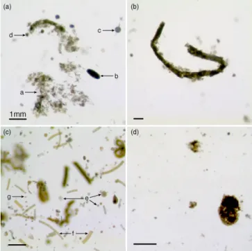
Particles collected in gels (Fig. 3) were phytodetrital ag-gregates (PA), cylindrical fecal pellets (CFP), oval fecal pel-lets, fecal aggregates (FA) and diatoms in the form of chains (e.g. the pennate Fragilariopsis spp.) or single cells (e.g. the centric Thalassiosira spp.). A few mesozooplankton speci-mens were collected (less than 10 per gel), and were mostly
Table 1. Deployment schedules for free-drifting sediment trap arrays.
Area Site ID Array Trap depths ±SD Event Time Latitude Longitude Duration Drift Tilt ± SD
(m) (m) (UTC)∗ (days) (km) (◦)
HNLC R-2 Gel traps 110, 210, 330, 430 0.8 Deploy 26 Oct 2011, 15:33 50◦21.580S 66◦42.930E 0.92 3.8 –
reference Recover 27 Oct 2011, 13:33 50◦20.100S 66◦40.690E
P trap 210 – Deploy 18 Oct 2011, 00:56 50◦42.570S 66◦41.470E – – –
Lost – – –
Off-plateau E-1 Gel traps 110, 210, 330, 430 1 Deploy 28 Oct 2011, 23:00 48◦28.720S 72◦12.680E 1.25 2.9 –
meander Recover 30 Oct 2011, 05:00 48◦27.480S 72◦11.270E
(time series) P trap 210 0. 6 Deploy 29 Oct 2011, 10:35 48◦29.660S 72◦14.280E 5.32 35 2.5 ± 0.7
Recover 3 Nov 2011, 18:14 48◦38.440S 71◦48.990E
E-3 Gel traps 110, 210, 430 0.9 Deploy 3 Nov 2011, 14:30 48◦41.920S 71◦57.890E 1.02 4 –
Recover 4 Nov 2011, 15:00 48◦43.900S 71◦56.660E
P trap 210 0.7 Deploy 5 Nov 2011, 07:52 48◦42.060S 71◦56.960E 5.11 43 0.3 ± 1
Recover 10 Nov 2011, 10:37 48◦40.770S 72◦32.080E
E-5 Gel traps 110, 210, 430 0.9 Deploy 18 Nov 2011, 13:50 48◦25.070S 71◦59.840E 1.06 10.1 – Recover 19 Nov 2011, 15:17 48◦30.250S 71◦57.420E
P trap 210 2.4 Deploy 18 Nov 2011, 14:42 48◦25.030S 71◦58.110E 1.55 15.1 4 ± 1.7
Recover 20 Nov 2011, 03:54 48◦33.160S 71◦56.860E
North polar F-L Gel traps 110, 210, 430 0.9 Deploy 6 Nov 2011, 14:30 48◦31.640S 74◦39.530E 0.92 14.2 –
front Recover 7 Nov 2011, 12:37 48◦36.600S 74◦48.400E
On-plateau A3-2 P trap (+gel) 210 (210) 1 Deploy 15 Nov 2011, 21:28 50◦37.800S 72◦4.810E 1.85 10.4 1 ± 0.9
reference Recover 17 Nov 2011, 17:46 50◦42.520S 72◦9.670E
∗
Times and locations are at the start of the deck operation.
represented by copepods (adult and copepodite stages) and appendicularians. Foraminifera and radiolarians were also occasionally observed. Phytodetrital aggregates were loose and green, while fecal aggregates contained dense, brown material. Most cylindrical fecal pellets had sharp edges and relatively constant diameters, but some were tapered along their length and had blurred edges composed of unpacked fecal material or attached phytodetritus (Fig. 3, panel b).
A preliminary image analysis was conducted to select the best analysis method in terms of particle identification. Parti-cles were classified into three main categories based on their significant contribution to the flux: phytodetrital aggregates, cylindrical fecal pellets and fecal aggregates. A fourth cat-egory, oval fecal pellets, was rare (less than one pellet per image in total), and its contribution to the flux was assumed negligible. Pictures were converted to binary images, with threshold levels adjusted manually on each picture to ensure a minimum alteration of particle areas. The average alteration of particle area estimated on a subsample was an increase of 21.6 ± 7 % (n = 169) for particles with irregular shapes (e.g. aggregates sensu lato including phytodetrital and fecal aggre-gates), and an increase of 11.6 ± 7 % (n = 44) for cylindri-cal fecylindri-cal pellets. Cylindricylindri-cal fecylindri-cal pellet and aggregate areas were systematically corrected for this overestimation.
Pictures were analysed with the US National Institutes of Health’s free software ImageJ. Typical shapes of each cate-gory of particle were determined manually on a subsample of particles. MATLAB routines using specific sets of shape descriptors were then applied to all images to identify and separate each category of particle. Because fecal and phy-todetrital aggregates had similar complex shapes, automated
Figure 3. High-resolution pictures of particles embedded in
poly-acrylamide gels showing the main categories of particles collected. Panel (a) – a: Phytodetrital aggregate; b: oval fecal pellet; b: ra-diolarian, d: foraminifera; panel (b) large cylindrical fecal pellet; panel (c) – e: small and large centric diatom single cells; f: chains of pennate diatoms of the genera Fragilariopsis spp., g: chain of small centric diatom cells; panel (d) fecal aggregate. Note the dif-ference in compactness and optical density between phytodetrital and fecal aggregates.
routines could not separate these particles efficiently. All fe-cal material was thus isolated manually from all other parti-cles based on the assumption that fecal matter is brown and denser than biologically unprocessed phytoplankton (Ebers-bach et al., 2011). From the resulting set of pictures, fecal ag-gregates were easily separated from cylindrical fecal pellets due to their very contrasted shapes. Tests on the efficiency of our automated selection, conducted on a large sample, showed that 93.4 % (n = 397) of cylindrical fecal pellets and 67.2 % (n = 171) of fecal aggregates were correctly identi-fied by the set of shape descriptors chosen.
All particle characteristics investigated in this study and their units are reported in Table 2. An area cut-off applied at 0.004 mm2 (0.07 mm equivalent spherical diameter) re-moved all “fake particles” deriving from small gel imperfec-tions and glass grid or microscope lens cleanliness. This cut-off removed 38 % of the total number of particles (mostly spurious particles and small single cells) but represented a loss of only 5.2 % of the total area of particles in the im-ages, introducing a negligible bias.
Aggregate area was converted to equivalent spherical di-ameter (ESD) assuming spherical shape, and the volume was calculated from the ESD. Because cylindrical fecal pellets were not always straight, their volume could not be accu-rately measured directly from their length and was calcu-lated from their perimeter and area (independent of pellet curvature), assuming a cylinder. The radius r of the cylin-der section was determined by finding the minimum root of the polynomial
4r2−P r + A =0, (1)
where P is the perimeter and A is the projected area of the aggregate. The length L was calculated from the projected area and radius using the formula
L = A/2r. (2)
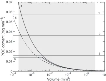
The volume was then calculated from the radius and length. The conversion from volume to carbon content was done by using different ratios and relationships depending on the particle considered. Figure 4 shows the relationship between carbon content and particle volume for different algorithms from the literature and those selected in this study. Based on values published by González and Smetacek (1994), the vol-ume of cylindrical fecal pellets was converted to their organic carbon content using a ratio of 0.036 mg C mm−3 (Fig. 4,
line 2), as an average value for copepod (Fig. 4, line 1), and euphausiid fecal pellets (Fig. 4, line 3). For fecal ag-gregates, we used the power relationship between POC con-tent and aggregate volume V , POC (µg) = 1.05V (mm3)0.51, based on the fractal decrease in carbon content with size and determined empirically by Alldredge (1998) for fecal marine snow (Fig. 4, line 4). The volume of phytodetrital aggregates was converted to carbon content using also a power rela-tionship determined by Alldredge (1998) for diatom marine
100−4 10−3 10−2 10−1 100 101 0.01 0.02 0.03 0.04 0.05 0.06 0.07 Volume (mm3) POC content (mg mm −3 ) 1 2 3 6 5 4
Figure 4. Empirical relationships of particulate organic carbon
(POC) content as a function of volume for different categories of sinking particles. 1, 2 and 3: copepod fecal pellets, average of eu-phausiids and copepod fecal pellets and eueu-phausiids fecal pellets respectively (González and Smetacek, 1994); 4: fecal marine snow (Alldredge, 1998); 5: diatom marine snow (Alldredge, 1998); 6: small and large aggregates (sensu lato) respectively (Ebersbach and Trull, 2008). The grey area represents the size range of particles pro-cessed in this study. Note the constant carbon mass per unit volume in fecal pellets based on solid geometry (linear relationship) and its decrease with increasing volume scaled on fractal geometry (power relationship) in the case of aggregates.
snow, POC (µg) = 0.97V (mm3)0.56 (Fig. 4, line 5), assum-ing aggregates composed of phytoplankton not biologically processed. In contrast to Ebersbach and Trull (2008; Fig. 4, line 6), very small particles (large single cells and aggregates composed of few cells) were included in the category of phy-todetrital aggregates and their volume-to-carbon conversion was done using the same relationship (Fig. 4, line 5).
Particle number and volume fluxes are presented in Sect. 3 as a function of size spectra. All particles were binned in 10 size classes spaced logarithmically to give the best represen-tation of the whole size range (Jackson et al., 1997, 2005). To avoid bias, bins containing five or fewer particles were not included in the flux spectrum analyses, as recommended by Jackson et al. (2005).
3 Results
3.1 Particles collected in polyacrylamide gel-filled sediment traps
3.1.1 Particle number, projected area and volume fluxes
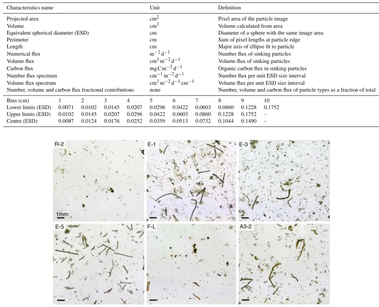
Despite variations in deployment duration among sites ex-ceeding 80 % (between 0.9 and 5.3 days, Table 1), an ob-servation of raw images (Fig. 5) gives a broad preliminary
Table 2. Particle characteristics and bins for phytodetrital aggregates, cylindrical fecal pellets and fecal aggregates.
Characteristics name Unit Definition
Projected area cm2 Pixel area of the particle image
Volume cm3 Volume calculated from area
Equivalent spherical diameter (ESD) cm Diameter of a sphere with the same image area
Perimeter cm Sum of pixel lengths at particle edge
Length cm Major axis of ellipse fit to particle
Numerical flux m−2d−1 Number flux of sinking particles Volume flux cm3m−2d−1 Volume flux of sinking particles
Carbon flux mg C m−2d−1 Organic carbon flux in sinking particles Number flux spectrum cm−1m−2d−1 Number flux per unit ESD size interval Volume flux spectrum cm3m−2d−1cm−1 Volume flux per unit ESD size interval
Number, volume and carbon flux fractional contributions none Number, volume and carbon flux of particle types as a fraction of total
Bins (cm) 1 2 3 4 5 6 7 8 9 10
Lower limits (ESD) 0.0071 0.0102 0.0145 0.0207 0.0296 0.0422 0.0603 0.0860 0.1228 0.1752 Upper limits (ESD) 0.0102 0.0145 0.0207 0.0296 0.0422 0.0603 0.0860 0.1228 0.1752 – Centre (ESD) 0.0087 0.0124 0.0176 0.0252 0.0359 0.0513 0.0732 0.1044 0.1490 –
Figure 5. Images of sinking particles embedded in polyacrylamide gels, collected at each site at 210 m. Comparison of images suggests
differences in terms of particles abundance and nature at each site.
indication on flux differences in terms of particle abundance (e.g. low fluxes at R-2 and F-L, and higher at E stations and A3-2). The lowest particle numbers, projected particle area and volume fluxes were collected at R-2 and F-L (Ta-ble 3 and Fig. 6), with particle volume fluxes of 2.5 ± 1 and 3 ± 0.7 cm3m−2d−1 respectively (all depths averaged). In contrast, high fluxes were collected at E stations with an av-erage volume flux of 7.5 ± 3 cm3m−2d−1(all E stations and depths averaged). Station A3-2 also presented a relatively high flux of 6.1 cm3m−2d−1.
Phytodetrital aggregates dominated in number at most sta-tions and depths (49 ± 10 % of the total number of parti-cles for all stations and depths averaged). Partiparti-cles not se-lected automatically as phytodetrital aggregates, cylindrical fecal pellets or fecal aggregates (“others” in Table 3)
repre-sented the second-largest numerical fraction (38 ± 8 %) but less than 9 % of the total projected particle area, and thus were assumed negligible in volume fluxes. Phytodetrital ag-gregates also dominated the volume fluxes (45.3 ± 22 %, all stations and depths averaged), with a maximum of 70 % at A3-2. However, volumes of cylindrical fecal pellets collected at E-5 (44 ± 33 %, all depths averaged) and volumes of fecal aggregates collected at F-L (57 ± 18 %, all depths averaged) represented the highest fractions at these stations.
Projected area fluxes at all stations and depths (Fig. 6) showed a clear attenuation of the total flux between 210 and 430 m (loss of 38 ± 21 % on average), with a maximum at-tenuation of 74 % at E-5 (Fig. 6a). A decrease in the flux of cylindrical fecal pellets with depth was combined with an in-crease in the flux of aggregates (mainly phytodetrital), except
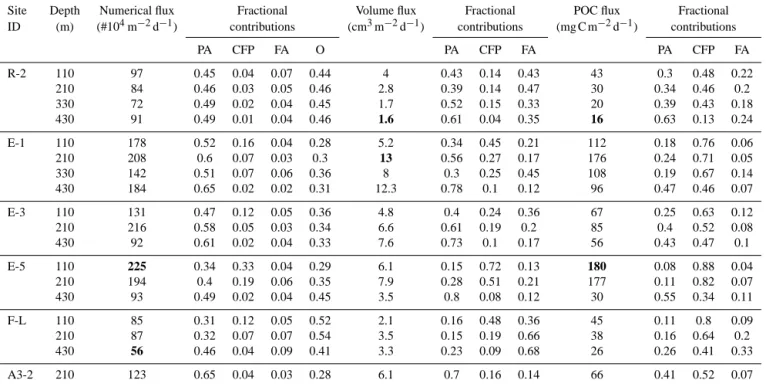
Table 3. Total numerical, volume and particulate organic carbon (POC) fluxes and fractional contributions of each category of particle.
Maximum and minimum fluxes are indicated in bold. PA: phytodetrital aggregates; CFP: cylindrical fecal pellets; FA: fecal aggregates; O: others.
Site Depth Numerical flux Fractional Volume flux Fractional POC flux Fractional ID (m) (#104m−2d−1) contributions (cm3m−2d−1) contributions (mg C m−2d−1) contributions
PA CFP FA O PA CFP FA PA CFP FA R-2 110 97 0.45 0.04 0.07 0.44 4 0.43 0.14 0.43 43 0.3 0.48 0.22 210 84 0.46 0.03 0.05 0.46 2.8 0.39 0.14 0.47 30 0.34 0.46 0.2 330 72 0.49 0.02 0.04 0.45 1.7 0.52 0.15 0.33 20 0.39 0.43 0.18 430 91 0.49 0.01 0.04 0.46 1.6 0.61 0.04 0.35 16 0.63 0.13 0.24 E-1 110 178 0.52 0.16 0.04 0.28 5.2 0.34 0.45 0.21 112 0.18 0.76 0.06 210 208 0.6 0.07 0.03 0.3 13 0.56 0.27 0.17 176 0.24 0.71 0.05 330 142 0.51 0.07 0.06 0.36 8 0.3 0.25 0.45 108 0.19 0.67 0.14 430 184 0.65 0.02 0.02 0.31 12.3 0.78 0.1 0.12 96 0.47 0.46 0.07 E-3 110 131 0.47 0.12 0.05 0.36 4.8 0.4 0.24 0.36 67 0.25 0.63 0.12 210 216 0.58 0.05 0.03 0.34 6.6 0.61 0.19 0.2 85 0.4 0.52 0.08 430 92 0.61 0.02 0.04 0.33 7.6 0.73 0.1 0.17 56 0.43 0.47 0.1 E-5 110 225 0.34 0.33 0.04 0.29 6.1 0.15 0.72 0.13 180 0.08 0.88 0.04 210 194 0.4 0.19 0.06 0.35 7.9 0.28 0.51 0.21 177 0.11 0.82 0.07 430 93 0.49 0.02 0.04 0.45 3.5 0.8 0.08 0.12 30 0.55 0.34 0.11 F-L 110 85 0.31 0.12 0.05 0.52 2.1 0.16 0.48 0.36 45 0.11 0.8 0.09 210 87 0.32 0.07 0.07 0.54 3.5 0.15 0.19 0.66 38 0.16 0.64 0.2 430 56 0.46 0.04 0.09 0.41 3.3 0.23 0.09 0.68 26 0.26 0.41 0.33 A3-2 210 123 0.65 0.04 0.03 0.28 6.1 0.7 0.16 0.14 66 0.41 0.52 0.07
at R-2, where a general flux attenuation was observed (all particle categories), and only a small increase in phytodetri-tal aggregates at 430 m.
Fluxes at E stations at 110 and 210 m decreased with time between E-1 and E-3, followed by a strong increase in cylin-drical fecal pellet flux at E-5 (Fig. 6c).
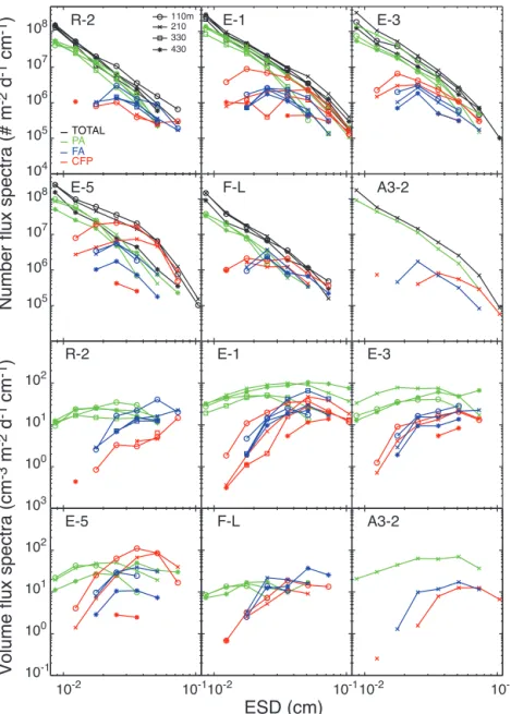
3.1.2 Number and volume flux spectra
Smallest particles were the most numerous at every site and depth (Fig. 7). Particle numbers decreased by more than 3 orders of magnitude for a 1 order of magnitude increase in size (0.008–0.07 cm), leading to slopes values around −3, and therefore in the range expected for particle size distri-bution (PSD) in natural waters (−2 to −5; Buonassissi and Dierssen, 2010; Guidi et al., 2009). Phytodetrital aggregates, representing the largest fraction of total particles, broadly followed the same spectra. Most cylindrical fecal pellets and fecal aggregates were middle-sized (ESD of 0.015–0.1 cm) with maximum abundances in the range 0.015–0.03 cm. E-5 presented the highest abundance of large fecal pellets (0.025 to 0.035 cm), with values exceeding 2 × 10⁷and 7 × 10⁶# m−2d−1cm−1at 110 and 210 m respectively.
At all sites, most of the volume flux of phytodetrital aggre-gates was carried by middle-sized particles (ESD of 0.01– 0.03 cm), due to the small contribution of large aggregates to the total number. Middle-sized and large cylindrical fecal pellets and fecal aggregates (ESD of 0.03–0.07 cm) carried
most of the volume flux, but again the largest particles did not bring the highest contribution due to their rarity relative to smaller particles (except at R-2, where the largest cylindri-cal fecylindri-cal pellets and fecylindri-cal aggregates contributed significantly to the volume flux).
The most notable change in the number flux spectra with depth was observed for middle-sized cylindrical fecal pellets at E stations, for which a decrease in number was generally combined with an increase in size. E-1 presents the best illus-tration, with most of the cylindrical fecal pellets with a size around 0.01 cm at 110 m increasing to 0.06 cm at 210 m. 3.1.3 POC flux from image analysis
The lowest carbon fluxes were estimated at R-2 and F-L (Ta-ble 3), with values of 27 ± 12 and 36 ± 10 mg C m−2d−1 re-spectively (all depths averaged). The highest carbon fluxes were observed at E stations (107 ± 33 mg C m−2d−1, all E stations and depths averaged), with a maximum value of 180 mg C m−2d−1at E-5, 110 m. A3-2 presented a moderate
carbon flux of 66 mg C m−2d−1at 210 m.
Cylindrical fecal pellets carried most of the carbon flux at all stations and depths, with an average fractional contri-bution of 56 ± 19 % (Table 3). This was particularly true at E stations, where fecal pellets drove on average 63 ± 17 % of the carbon flux (maximum of 88 % at E-5, 110 m), and at F-L (62±20 %, all depths averaged). However, at several stations, a transition was observed at 430 m, where phytodetrital
ag-R-2 E-1 E-3 E-5 F-L A3-2 Stations 0 200 400 600 800 R-2 E-1 E-3 E-5 F-L A3-2
Projected area flux (cm0 200 400 600 8002 m−2 d−1)
110 m 210 m 330 m 430 m Stations TOTAL (((( (( PA CFP FA
(a)
(b)
(c)
(d)
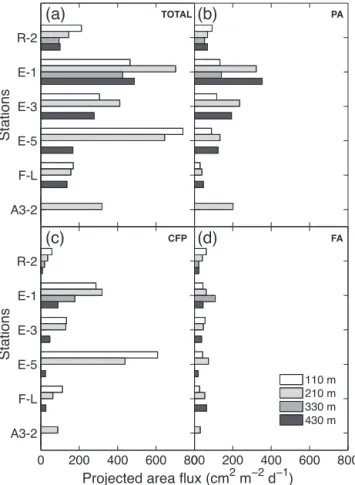
Figure 6. Projected area of particles estimated from image
analy-sis at each site and depth and expressed as fluxes (cm2m−2d−1).
(a) All particles (TOTAL), (b) phytodetrital aggregates (PA), (c)
cylindrical fecal pellets (CFP) and (d) fecal aggregates (FA). The figure suggests a sinking flux dominated by cylindrical fecal pellets at the surface, except at R-2, where phytodetrital aggregates repre-sented the most important fraction. The attenuation of the cylindri-cal fecylindri-cal pellet flux with depth observable at all stations was com-bined with an increase in the flux of phytodetrital and fecal aggre-gates at almost all stations. At 430 m, phytodetrital aggreaggre-gates were then the most dominant particles.
gregates brought the largest fractional contribution with 63, 47 and 55 % at R-2, E-1 and E-5 respectively. Fecal aggre-gates generally carried a small fraction of the carbon flux, with an average of 13±8 % (all stations and depths), but their contribution tended to increase with depth (e.g. 24 and 33 % at 430 m at R-2 and F-L respectively).
3.2 Biogeochemical fluxes collected in PPS3/3 traps
Bulk fluxes from PPS3/3 traps are reported in Table 4. The highest mass, POC, 234Th and TPN fluxes were collected at E stations. POC fluxes decreased over time from 84 ± 27 at E-1, to 58 ± 18 at E-3, to 24 ± 12 at E-5 mg C m−2d−1. A3-2 presented a POC flux of 27 mg C m−2d−1. An average
234Th activity of 988 ± 127 dpm m−2d−1was recorded at E
stations, with a maximum of 1129 ± 177 dpm m−2d−1at
E-3.234Th fluxes are detailed in Planchon et al. (2014). Over all sites, BSi fluxes were very high (7 ± 2 to 21 ± 10 mmol BSi m−2d−1), suggesting the large contribution of diatoms
to the phytoplankton community. Conversely, very low par-ticulate inorganic carbon (PIC) fluxes (1–4 orders of mag-nitude lower than POC fluxes) suggested the limited role of calcium carbonate (CaCO3) in biogenic mineral fluxes.
POC : TPN ratios were close to the canonical Redfield ra-tio of 6.6 for phytoplankton at all stara-tions except E-5 (7.5), which also displayed the lowest POC : BSi ratio (0.1). At E stations, POC :234Th and POC : mass ratios decreased over time (POC :234Th ratios from 8 at E-1 to 2.1 µmol dpm−1 at E-5; POC : mass ratio from 0.05 at E-1 to 0.03 g g−1 at E-5), suggesting an attenuation of export fluxes com-bined with a degradation of sinking particles. A3-2 displayed POC :234Th and POC : mass ratios of 4.4 µmol dpm−1 and 0.06 g g−1respectively. In general, no consistent differences
in fluxes could be resolved between poisoned and unpoi-soned cups.
3.3 POC flux comparisons and export efficiencies
POC fluxes determined from gel images (using particle volume-to-carbon-content conversion factors) were in the same range of values as those determined from particle col-lection in PPS3/3, with maximum differences at a same sta-tion never exceeding 1 order of magnitude (Tables 3 and 4). POC fluxes from PPS3/3 were systematically lower than those derived from image analysis (on average 57 ± 22 % less).
E-ratios, calculated as the ratio of POC fluxes from gel im-age analysis to 1 % PAR-integrated net primary productivity (Cavagna et al., 2014; Table 5) indicated a high export effi-ciency at R-2 and E-1 (0.2±0.08 and 0.23±0.07 respectively, all depths averaged), intermediate at E-3 and E-5 (0.1 ± 0.02 and 0.13 ± 0.09 respectively, all depths averaged), and very low at F-L (0.01 ± 0.0, similar value at all depths) and A3-2 (0.03). E-ratios derived from POC fluxes estimated from PPS3/3 traps showed lower values but followed the same trend: E-1 > E-3 > E-5 > A3-2. Export efficiencies derived from234Th disequilibria, ThEC(Planchon et al., 2014), are
shown in Table 5 for comparison, and are discussed in the next section.
According to calculations based on gel trap POC flux and transmissometer POC concentration estimates (Fig. 2), E sta-tions exported the largest percentage of their mixed-layer-integrated POC (6POCML) per day (2.4 ± 1 %, all E
sta-tions and depths averaged) with the maximum observed at E-5 (2.7 ± 1.8 %, all depths averaged) and values of 2.3 ± 0.7 and 2.3 ± 0.5 % at E-1 and E-3 respectively (all depths av-eraged). R-2 and F-L exported respectively 0.58 ± 0.2 and 0.59 ± 0.15 % of their 6POCML per day (all depths
aver-aged), and A3-2 exported 0.32 % of its 6POCML per day
(210 m). A similar trend was obtained using POC fluxes from PPS3/3 traps (E stations > A3-2).
10-110-2 10-110-2 10-1 102 101 100 10-1 101 100 103 106 105 107 108 106 105 104 107 108
Number flux spectra (# m
-2
d
-1cm
-1)
110m210 330 430 102Volume flux spectra (cm
-3
m
-2d
-1cm
-1)
10-2ESD (cm)
PA FA CFP TOTAL R-2 E-1 E-3 E-5 F-L A3-2 R-2 E-1 E-3 E-5 F-L A3-2Figure 7. Total number and volume fluxes of particles binned in 10 size classes. Bins with less than five particles were removed (see Table 2
and text for explanations). Results are shown for each category of particles at all depths and sites. TOTAL: all particles; PA: phytodetrital aggregates; FA: fecal aggregates; CFP: cylindrical fecal pellets. Smallest particles represented by phytodetrital aggregates were the most numerous at every site and depth. Middle-sized phytodetrital aggregates and fecal particles (pellets and aggregates) contributed the most to the volume flux due to the overall rarity of very large particles relative to all particles.
4 Discussion
4.1 Comparison of POC flux estimations
Two different approaches were used to estimate POC fluxes. PPS3/3 trap collection providing a direct determination of the flux served as a reference method. POC fluxes esti-mated from image analysis of particles embedded in poly-acrylamide gels were in the same range as those derived from PPS3/3 but were systematically higher (see Sect. 3). This difference is most likely due to the uncertainty in the volume-to-carbon conversion factors (Fig. 4) used to
esti-mate POC fluxes from particle image analysis. A compar-ison with the direct estimation of bulk fluxes collected in PPS3/3 suggests that our volume-to-carbon-content conver-sion factors tended to slightly overestimate the carbon car-ried by sinking particles (Tables 3 and 4), especially at E-5, where it was up to 7-fold higher. At this station the large contribution of cylindrical fecal pellets to the volume flux (Table 3; 72 % at 110 m and 51 % at 210 m) suggests that the volume-to-carbon conversion factor used for these particles may be responsible for the mismatch observed. The value of 0.036 mg C mm−3 used as an average for copepod and
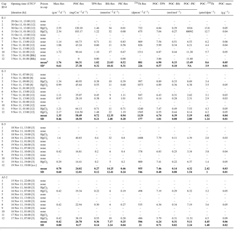
con-Table 4. Particle fluxes at 210 m depth from free-drifting deployments of the 12-cup-carousel cylindrical PPS3/3 trap. The trap collection
area was 0.125 m2. Particles were washed through a 350 µm Nitex screen to remove zooplankton and were collected on a 1 mm silver filter. Mean values and their standard deviations are indicated in bold.
Cup Opening time (UTC)a Poison Mass flux POC flux TPN flux BSi flux PIC flux 234Th flux POC : TPN POC : BSi POC : PIC POC :234Th POC : mass
ID # in cup
[duration (h)] (g m−2d−1) (mg C m−2d−1) (mmol m−2d−1) (dpm m−2d−1) (mol mol−1) (µmol dpm−1) (g g−1) E-1 1 29 Oct 11, 13:00 [12] none – – – – – – – – – – – 2 30 Oct 11, 01:00 [12] none – – – – – – – – – – – 3 30 Oct 11, 13:00 [12] HgCl2 2.55 120.10 1.46 34 0.01 722 6.84 0.29 1016 13.8 0.05 4 31 Oct 11, 01:00 [12] HgCl2 2.34 103.17 1.22 32 0.00 675 7.04 0.27 88092 12.7 0.04 5 31 Oct 11, 13:00 [12] none – – – – – – – – – – – 6 1 Nov 11, 01:00 [12] none – – – – – – – – – – – 7 1 Nov 11, 13:00 [12] none 1.14 64.73 0.71 11 0.83 869 7.56 0.51 6.53 6.2 0.06 8 2 Nov 11, 01:00 [12] none 1.06 43.24 0.60 11 0.58 826 5.99 0.34 6.21 4.4 0.04 9 2 Nov 11, 13:00 [12] none – – – – – – – – – – – 10 3 Nov 11, 01:00 [12] none 1.72 90.44 1.10 17 0.67 1311 6.87 0.44 11.30 5.7 0.05 11 3 Nov 11, 01:00 [Blk] none – – – – – – – – – – – 12 3 Nov 11, 01:00 [Blk] none – 0 0.00 – 0.00 – 3.86 – 11.60 – – meanb 1.76 84.31 1.02 21.03 0.52 881 6.90 0.33 13.49 8.6 0.05 SDc 0.61 27.38 0.32 10.41 0.31 226 0.57 0.10 NA 3.9 0.01 E-3 1 5 Nov 11, 07:00 [1] none – – – – – – – – – – – 2 5 Nov 11, 08:00 [8] none – – – – – – – – – – – 3 5 Nov 11, 09:00 [1] HgCl2 1.34 40.95 0.38 10 0.39 997 8.89 0.33 8.69 3.4 – 4 5 Nov 11, 17:00 [8] HgCl2 0.99 45.64 0.55 11 0.60 1073 6.89 0.36 6.38 3.5 0.05 5 6 Nov 11, 01:00 [12] none – – – – – – – – – – – 6 6 Nov 11, 13:00 [12] none – – – – – – – – – – – 7 7 Nov 11, 01:00 [12] none 1.11 35.07 0.45 9 1.11 947 6.43 0.31 2.62 3.1 0.03 8 7 Nov 11, 13:00 [12] none 0.97 28.10 0.38 8 1.01 813 6.14 0.28 2.31 2.9 0.03 9 8 Nov 11, 01:00 [12] none – – – – – – – – – – – 10 8 Nov 11, 13:00 [12] none – – – – – – – – – – – 11 9 Nov 11, 01:00 [12] HgCl2 1.21 64.13 0.71 11 0.71 1240 7.47 0.49 7.53 4.3 0.05 12 9 Nov 11, 13:00 [12] HgCl2 2.17 116.50 1.48 22 1.19 1565 6.55 0.44 8.14 6.2 0.05 mean 1.35 58.49 0.72 12.35 0.94 1129 6.74 0.39 5.19 4.02 0.04 SD 0.46 18.50 0.21 2.48 0.20 177 1.01 0.08 2.80 1.24 0.01 E-5 1 18 Nov 11, 13:00 [3] none – – – – – – – – – – – 2 18 Nov 11, 16:00 [3] none – – – – – – – – – – – 3 18 Nov 11, 19:00 [3] HgCl2 – – – – – – – – – – – 4 18 Nov 11, 22:00 [3] HgCl2 1.6 40.83 0.4 32 0.8 1688 7.79 0.11 4.39 2.0 0.03 5 19 Nov 11, 01:00 [3] none – – – – – – – – – – – 6 19 Nov 11, 04:00 [3] none – – – – – – – – – – – 7 19 Nov 11, 07:00 [3] none – – – – – – – – – – – 8 19 Nov 11, 10:00 [3] none 0.42 16.81 0.2 6 0.4 378 6.83 0.25 3.34 3.8 0.04 9 19 Nov 11, 13:00 [3] none – – – – – – – – – – – 10 19 Nov 11, 16:00 [3] none – – – – – – – – – – – 11 19 Nov 11, 19:00 [3] HgCl2 0.29 14.41 0.2 5 0.2 800 7.41 0.22 6.37 1.4 0.05 12 19 Nov 11, 19:00 [n.r.] – – – – – – – – – – – – mean 0.78 24.02 0.27 14.25 0.46 955 7.46 0.14 4.32 2.42 0.03 SD 0.60 12.01 0.12 12.41 0.24 546 0.48 0.08 1.54 1 0.01 A3-2 1 15 Nov 11, 22:00 [3] none – – – – – – – – – – – 2 16 Nov 11, 01:00 [3] none – – – – – – – – – – – 3 16 Nov 11, 04:00 [3] HgCl2 – – – – – – – – – – – 4 16 Nov 11, 07:00 [3] HgCl2 0.42 19.34 0.22 6 0.19 498 7.19 0.29 8.32 3.2 0.05 5 16 Nov 11, 10:00 [3] none – – – – – – – – – – – 6 16 Nov 11, 13:00 [3] none – – – – – – – – – – – 7 16 Nov 11, 16:00 [3] none – – – – – – – – – – – 8 16 Nov 11, 19:00 [3] none 0.42 22.94 0.30 6 0.27 535 6.36 0.34 7.19 3.6 0.05 9 16 Nov 11, 22:00 [3] none – – – – – – – – – – – 10 16 Nov 11, 01:00 [3] none – – – – – – – – – – – 11 17 Nov 11, 04:00 [3] HgCl2 – – – – – – – – – – – 12 17 Nov 11, 07:00 [3] HgCl2 0.42 38.19 0.55 10 0.28 486 5.79 0.31 11.51 6.5 0.09 mean 0.42 26.78 0.36 7.17 0.25 506 6.24 0.31 9.11 4.45 0.06 SD 0.00 8.17 0.14 2.24 0.04 21 0.71 0.02 2.24 1.48 0.02
aLocal time was UTC + 5 h.
bFor all stations, mean values are the total collection divided by the total time over the entire deployment.
cFor all stations, flux standard deviations are weighted by cup duration times. Component ratio standard deviations are unweighted. n.r.: not rotated.
NA: not available. Blk: blank.
tained in the cylindrical fecal pellets collected. Feeding be-haviours (e.g. herbivorous or coprophagous) specific to each zooplankton group will produce fecal pellets with variable carbon content due to variable fraction of undigested food, compaction or vulnerability to physical or biological degra-dation (Urban-Rich et al., 1998). Constant carbon to volume ratios are thus unable to reflect the myriad of fecal pellet
compositions linked to ecosystem structure variations. Val-ues of carbon content in cylindrical fecal pellets found in the literature range over approximately 1 order of magnitude between 0.01 and 0.1 mg C mm−3(González and Smetacek, 1994; González et al., 1994, 2000; Carroll et al., 1998), lead-ing to potential strong variations in carbon flux estimations if large volumes of fecal pellets are involved, as was the case at
Table 5. Export efficiency at each site estimated from several
meth-ods. Maximum and minimum export efficiencies are indicated in bold.
Site Depth E-ratios ThEC %P POCMLexport 1 d
ID (m) Gels PPS3/3 Gels PPS3/3 R-2 100 ± 10 0.32 – 0.34 0.92 – 200 ± 10 0.22 – 0.16 0.64 – 330 0.15 – – 0.43 – 430 0.12 – – 0.34 – E-1 100 ± 10 0.21 – 0.27 2.12 – 200 ± 10 0.34 0.16 ±0.05 0.18 3.34 1.59 ± 0.52 330 0.21 – – 2.05 – 430 0.18 – – 1.82 – E-3 100 ± 10 0.10 – 0.21 2.22 – 200 ± 10 0.12 0.08 ± 0.03 0.14 2.82 1.92 ± 0.64 430 0.08 – – 1.86 – E-5 100 ± 10 0.19 – 0.11 3.76 – 200 ± 10 0.19 0.03 ± 0.02 0.1 3.69 0.50 ± 0.25 430 0.03 – – 0.63 – F-L 100 ± 10 0.01 – 0.01 0.73 – 200 ± 10 0.01 – 0.01 0.62 – 430 0.01 – – 0.42 – A3-2 100 ± 10 – – 0.05 – – 200 ± 10 0.03 0.01 ±0.004 0.02 0.32 0.13 ± 0.04
E-ratio: POC flux (gels, PPS3/3) / NPP (EZintegration 1 % PAR; data from Cavagna et al., 2014). ThEC: POC flux (234Th; data from Planchon et al., 2014) / NPP.
%P POCMLexport 1 d: percentage of mixed-layer-integrated POC exported in 1 day.
E-5. Mesozooplankton communities collected in Bongo nets from 250 m to the surface (day and night haulings, except at R-2 and F-L, where only day haulings were conducted), and analysed with a ZooScan integrated system (Carlotti et al., 2015), generally revealed a large dominance of the size fraction 500–1000 µm with values from 54 to 79 % (consider-ing only the stations where the traps were deployed). Micro-scopic identifications confirmed a community largely domi-nated by copepods (Carlotti et al., 2015). However, most of the fecal pellets collected in gel traps at E-5 were large frag-ments (Fig. 5), with a peritrophic membrane interrupted at their extremities suggesting more probably an origin from euphausiids rather than copepods, which produce smaller fe-cal pellets with a continuous peritrophic membrane termi-nated by a pellicle (Gauld, 1957; Martens, 1978; Yoon et al., 2001). Differences in euphausiid and copepod fecal pel-let sinking velocities due to size variations, ballast content or compaction (Fowler and Small, 1972; Small et al., 1979), as well as contrasted sensitivities to degradation or zooplankton vertical migration behaviours (Wallace et al., 2013), could explain the mismatch between the zooplankton community identified from net haulings and the fecal pellets collected in gel traps. A reduced collection efficiency of euphausiids compared to copepods could also be responsible for this mis-match, knowing that specific nets like the Multiple Opening and Closing Nets and Environment Sensing System (MOC-NESS; Wiebe et al., 1976) are needed to efficiently capture both mesozooplankton and euphausiids in the layer 0–250 m (e.g. Espinasse et al., 2012). Most studies show that
zoo-plankton net avoidance is complex and variable; it depends on environmental conditions (e.g. light regime), net charac-teristics, and various zooplankton characcharac-teristics, including size, shape, species, sex and developmental stage (Brinton, 1967; Fleminger and Clutter, 1965; Wiebe et al., 1982).
Assuming a dominance of euphausiid fecal pellets at E-5, the use of the reference value of 0.016 mg C mm−3improves the match between POC fluxes estimated from PPS3/3 and gel traps (ratios POCgels/POCPPS3/3=4), although it
can-not fully explain the discrepancy, presumably due to other factors (e.g. particle field heterogeneity or small differences in sediment trap collection efficiencies).
4.2 Evolution of the flux at depth
POC fluxes presented in Fig. 8 were estimated through two different approaches: gel trap image analysis (at 110, 210, 330 and 430 m) and total 234Th activity measured at 11– 14 depths at all stations (Planchon et al., 2014) and calcu-lated at 100, 150 and 200 m. Fluxes estimated from PPS3/3 trap collection at only one depth (210 m) are not presented here. Figure 8 shows the evolution of POC fluxes with depth and its comparison with the empirical flux attenuation known as the “Martin curve” (Martin et al., 1987), estimat-ing the flux at depth from values at 100 m rangestimat-ing from 20 to 500 mg C m−2d−1. Agreements between POC flux determi-nation methods and this empirical relationship were the best for R-2 and F-L, showing a continuous attenuation of the flux with depth, but always at a lower rate than predicted by the Martin curve.
For all other stations POC fluxes above 210 m presented complex patterns suggesting distinct POC export episodes to be more likely than a continuous downward flux. Between 210 and 430 m the attenuation of POC fluxes estimated from the gel traps tends to be more consistent with the Martin curve, except for E-5, which displayed a strong decrease (as already noted in the Sect. 3). A fecal pellet loss at depth was particularly strong at E-5, due to the large role played by these particles at this site, but was observed at all stations (Fig. 6).
Our data revealed two major trends of particle flux evo-lution with depth: (i) the fecal pellet flux decreased, and (ii) phytodetrital and fecal aggregate fluxes remained con-stant or even increased. Establishing a link between these two processes is tempting. It suggests the importance of physical reaggregation in sustaining the carbon flux at depth from fecal pellets that have undergone bacterial degradation or zooplankton coprorhexy (Suzuki et al., 2003; Lampitt et al., 1990; Iversen and Poulsen, 2007). A recent study from Giering et al. (2014) suggests that half of fast-sinking par-ticles in the twilight zone of the eastern Atlantic Ocean (between 50 and 1000 m) are fragmented and ingested by zooplankton, and that more than 30 % may be released as suspended and slowly sinking organic matter. Even if the gel trap technique does not offer enough information on
101 102 100 150 200 250 300 350 400 450 Carbon flux (mg C m−2 d−1) Depth (m) R-2 F-L E-5 E-3 E-1 20 500 45 100 224 234Th Gel trap Martin et al. (1987) A3-2
Figure 8. Variation in the carbon flux with depth estimated from gel
trap and234Th methods. The empirical attenuation of the flux with depth (Martin curve) is represented by grey dashed lines for initial values of the carbon flux at 100 m from 20 to 500 mg C m−2d−1. Results show overall poor agreements between observed fluxes and the Martin curve, suggesting the complexity of the processes affect-ing the carbon flux with depth.
aggregation processes and particle sources to permit any clear conclusion, the hypothesis of a reaggregation of un-packed fecal pellets into “secondary” phytodetrital aggre-gates still deserves careful consideration.
Since the rate of physical aggregation is largely controlled by particle concentration (Jackson, 1990), a reaggregation at depth implies that sufficient material has been released by fe-cal pellet disaggregation. If single cells represented most of the material released during fecal pellet disaggregation, their concentration should have increased with depth in the case of no secondary aggregation or remained constant as a balance between aggregate formation and loss by sinking (notion of critical concentration; Jackson, 1990, 2005). The number flux spectra (Fig. 7) suggest that the smallest particles had a constant concentration until 210 m at almost every site. Sta-tion E-3 shows an increase in the number of small particles between 110 and 210 m and then a decrease at 430 m, which could indicate reaggregation processes occurring at depth. This decrease at 430 m is also observable at E-5 and F-L. However, data evaluation in this way implies a steady-state assumption which considers that traps measured the occur-rence of a unique sinking event; the flux collected at depth being a direct temporal evolution of the same shallower flux. This appears unlikely considering the episodic nature of ex-port and its dependence on highly dynamical ecosystem in-teractions responsible for high flux variability at short spatio-temporal scales as evidenced by the PPS3/3 individual cup
(a)
(b)
2 2.5 3 3.5 0 0.1 0.2 0.3 0.4 0.5 Log[NPP(mg C m−2 d−1)] Export efficiency 0 50 100 150 200 250 300 0 0.1 0.2 0.3 0.4 Zooplankton biomass (mm3 m−3) Export efficiency k2 gels k2 PPS3/3 k1 gels k1 PPS3/3 Maiti et al.(2013) k1 & 2 k2 234Th k1 234Th E-3Figure 9. Relationships between net primary productivity (a),
zoo-plankton biomass (b) and export efficiency calculated using partic-ulate organic carbon fluxes estimated at 200 ± 10 m from PPS3/3 traps, gel traps and 234Th methods for the KEOPS2 (k2) and KEOPS1 (k1, (a) only) studies. (a) The black line represents the em-pirical relationship from Maiti et al. (2013) estimated in the South-ern Ocean (y = −0.35x +1.22; r2=0.97), and the dashed line rep-resents the regression line for all KEOPS data (y = −0.19x + 0.68;
n =24, r2=0.33, p < 0.005). (b) The dashed line represents the regression line for KEOPS2 data (y = −0.00086x+0.2232; n = 15,
r2=0.72, p < 0.0005). E-3 was assumed an outlier and was ex-cluded from the best fit calculation (see text for possible expla-nation). Panel (a) suggests that the most productive sites are the less efficient to export carbon. Panel (b) suggests that zooplankton biomass could influence the efficiency of carbon export by bypass-ing direct export via phytodetrital aggregates.
variations (Table 4). In addition, if assuming phytodetrital ag-gregates at E-3, sinking at an average velocity of 150 m d−1
(based on results from Laurenceau-Cornec et al., 2015), a particle field would need approximately 1.5 days to sink from 210 to 430 m, neglecting any advection. Considering this cal-culation and the short trap deployment at E-3 (1.02 days), a non-steady-state assumption appears more reasonable, and the increase in phytodetrital and fecal aggregates observed at depth could reflect an earlier production event.
4.3 Temporal POC flux variations during KEOPS2 and comparison with KEOPS1
From E-1 to E-5, the POC flux varied with the depth and es-timation method. Collection of POC flux in PPS3/3 trap at 210 m revealed a monotonic decrease in the flux with time (Table 4). Temporal evolution of the flux between E-1, E-3 and E-5, at 100±10 and 200±10 m, using gel trap and234Th methods (Planchon et al., 2014), shows a almost constant flux (undistinguishable differences within the uncertainties). At 430 m, gel traps measured flux evolutions comparable to those identified in the PPS3/3 at 210 m, i.e. a continuous de-crease in the flux with time. With the results from 110 and 210 m at E-5 excluded (likely linked to an episodic flux of euphausiid fecal pellets at these depths; see text above), the gel traps also show a decrease in the total flux over time, consistent with PPS3/3 trap method. The unusual increase at E-5, against the steady background of the other E stations, highlights the importance of zooplankton in modifying the particle flux.
At the KEOPS1 (January–February 2005) bloom refer-ence station A3, POC flux values estimated at 200 m from gel trap image analysis and PPS3/3 traps were 62 and 13– 20 mg C m−2d−1 respectively (Ebersbach and Trull, 2008), i.e. in the same range as during KEOPS2 at the same sta-tion and using the same methods (gels: 66 mg C m−2d−1; PPS3/3: 27 mg C m−2d−1). During KEOPS1, the 234 Th-based method assuming a non-steady-state system (NSS) yielded 200 m POC fluxes of 294 mg C m−2d−1 at A3 (flux averaged over 21 days) and 124 mg C m−2d−1 at the KEOPS1 HNLC reference station C11 (flux averaged over 10 days; Savoye et al., 2008). These values are well above the KEOPS2 values of 46 and 22 mg C m−2d−1determined
at 200 m at A3-2 and R-2 respectively using the same method (average over 28 days, except for R-2 assumed in steady state; Planchon et al., 2014). The 234Th-based method as-suming NSS integrated the POC flux over a period longer than 20 days, contrasting with the 1 day to 1 week period provided by gel and PPS3/3 trap estimations.
Seasonal trends are more reliable if calculated over a longer period, and the234Th-based method then gives the best insight into the temporal evolution of the POC flux from the onset of the bloom to its decline.234Th results suggest that the POC flux was approximately 5- to 6-fold higher at the decline of the bloom (January–February) than dur-ing its onset (October–November), agreedur-ing with the com-mon view that most of the export flux occurs in late bloom stage (Wassmann, 1998). During KEOPS1, at A3 and C11, the NPP integrated within the euphotic zone was 1030 ± 43 and 224±30 mg C m−2d−1respectively (based on13C incor-poration; Mosseri et al., 2008; Lefèvre et al., 2008). In com-parison, values of 1903±186 and 135±6 mg C m−2d−1were determined at A3-2 and R-2 during KEOPS2 (euphotic zone, EZ 1 % PAR-integrated NPP based on 13C incorporation;
Cavagna et al., 2014). Carbon export efficiencies estimated
at 200 m, based on234Th-derived POC export flux (reported
as ThEC), were 30 % at A3 and 49 % at C11 during KEOPS1
(calculations using data from Savoye et al., 2008; Mosseri et al., 2008). In contrast, ThECvalues of 2 % (NSS model) and
16 % (SS model) were calculated at 200 m at A3-2 and R-2 respectively during KEOPS2 (Planchon et al., 2014). These results show that (i) primary productivity at the on-plateau site was approximately 2-fold higher in spring than during summer and (ii) carbon export fluxes were approximately 5-fold lower during early than late bloom stage, leading to (iii) carbon export efficiencies up to 10-fold lower during the early bloom stage (spring) than during late bloom stage (summer).
4.4 Toward an explanation of the negative relationship between primary productivity and carbon export efficiency
We examined two different export efficiency indicators (Ta-ble 5): (i) e-ratios calculated as the ratio between POC fluxes estimated from gel images or PPS3/3 traps, and net primary productivity integrated over the euphotic zone (EZ1 % PAR;
Cavagna et al., 2014), and (ii) ThEC calculated as the ratio
between POC flux estimated from234Th method and net pri-mary productivity. KEOPS2 results suggest a negative rela-tionship between primary productivity and carbon export ef-ficiency, the most productive sites being those where carbon is exported the least efficiently. Figure 9a shows the rela-tionship between primary productivity and export efficiency (with POC fluxes estimated at 200 ± 10 m from gels, PPS3/3 traps and 234Th water column disequilibria) for KEOPS2 sites. For comparison purposes, KEOPS1 data are also in-dicated (Savoye et al., 2008). The empirical relationship pro-posed recently by Maiti et al. (2013), based on surface teth-ered cylindrical sediment traps and234Th data from up to 130 stations in the Southern Ocean, is also reported. While this negative relationship has now been observed in several field studies in the Southern Ocean (Savoye et al., 2008; Morris et al., 2007; Jacquet et al., 2011), and elsewhere (e.g. González et al., 2009), the reasons for its existence remain unclear. Maiti et al. (2013) mentioned differences in trophic structure, grazing intensity, recycling efficiency, high bacterial activity, or increase in DOC export as possible explanations for high-productivity, low-export-efficiency regimes. Phytoplankton physiological state has also been suggested as a possible con-trol of carbon export mode and efficiency (González et al., 2009), although this could not be verified here due to a gen-erally good phytoplankton physiological state confirmed via microscopy over the course of the KEOPS2 study (M. Las-bleiz and K. Leblanc, personal communication, 2014). In ad-dition, due to their degradation-resistant and heavily silicified valves (Hargraves and French, 1983; Kuwata and Takahashi, 1990), the abundance of diatom resting spores in the sink-ing flux, as observed dursink-ing KEOPS1 (Armand et al., 2008), could also be a major factor to consider when evaluating