HAL Id: hal-00614186
https://hal.archives-ouvertes.fr/hal-00614186
Submitted on 10 Aug 2011
HAL is a multi-disciplinary open access
archive for the deposit and dissemination of sci-entific research documents, whether they are pub-lished or not. The documents may come from teaching and research institutions in France or abroad, or from public or private research centers.
L’archive ouverte pluridisciplinaire HAL, est destinée au dépôt et à la diffusion de documents scientifiques de niveau recherche, publiés ou non, émanant des établissements d’enseignement et de recherche français ou étrangers, des laboratoires publics ou privés.
To cite this version:
Gabriel Reygondeau, Gregory Beaugrand. Water column stability and Calanus finmarchi-cus. Journal of Plankton Research, Oxford University Press (OUP), 2010, 33 (1), pp.119. �10.1093/plankt/FBQ091�. �hal-00614186�
For Peer Review
Water column stability and Calanus finmarchicus
Journal: Journal of Plankton Research
Manuscript ID: JPR-2010-033.R1
Manuscript Type: Original Article
Date Submitted by the
Author: 05-Jun-2010
Complete List of Authors: Reygondeau, Gabriel; Institut de la recherche et du devellopement, Ecologie milieu expoloité EME 212
Beaugrand, Gregory; Alister Hardy Foundation for Ocean Science, Citadel Hill, the Hoe
Keywords: thermocline, Calanus finmarchicus , North Atlantic Ocean , Macroecology, Exponentially Weighted Moving Average
For Peer Review
Water column stability and Calanus finmarchicus
Gabriel Reygondeau 1, Grégory Beaugrand 2,3 1IRD (Institut de Recherche pour le Développement)
UMR EME 212, CRH (Centre de Recherches Halieutiques Méditerranéennes et Tropicales) av. Jean Monnet, B.P. 171, 34203 Sète cedex, FRANCE,
E-mail: [email protected]
2 Centre National de la Recherche Scientifique, Laboratoire d’Océanologie et de Géosciences’ UMR LOG CNRS 8187, Station Marine, Université des Sciences et Technologies de Lille –
Lille 1
BP 80, 62930 Wimereux, France, E-mail: [email protected]
3
Sir Alister Hardy Foundation for Ocean Science, Citadel Hill, the Hoe, Plymouth PL1 2PB, United Kingdom
* To whom correspondence should be addressed. E-mail: [email protected]
3 4 5 6 7 8 9 10 11 12 13 14 15 16 17 18 19 20 21 22 23 24 25 26 27 28 29 30 31 32 33 34 35 36 37 38 39 40 41 42 43 44 45 46 47 48 49 50 51 52 53 54 55 56 57 58 59 60
For Peer Review
Abstract
Many authors have suggested that the abundance of the subarctic species Calanus finmarchicus can be influenced by the structure of the water column. Unfortunately to date, such a link has never been confirmed either experimentally or statistically. By using a macroecological approach, we investigated this hypothesis and showed that it varies with the developmental stage of the species. First, we implemented a new statistical procedure, based on an exponentially weighted moving average, to identify and quantify the depth and intensity of the thermocline. We applied the technique on 1,005,619 temperature profiles over the North Atlantic Ocean and provide a mapping of these two descriptors at a seasonal scale. Second, we studied the relationships between the depth and the intensity of the thermocline and Calanus finmarchicus using a biological dataset of 99,599 sampling stations. Our results suggested that the characteristics of the water column influence the spatial distribution of C. finmarchicus. The frequency in the occurrence of this species decreases when stratification rises. Our results further revealed that the effect is more pronounced for young copepodite stages. Such findings are of interest since, in a warmer world, water stratification is expected to increase, making more likely a reduction in the abundance of this key species in the North Atlantic.
Key-words: Exponentially Weighted Moving Average; Calanus finmarchicus; thermocline ;
North Atlantic Ocean; Macroecology
2 3 4 5 6 7 8 9 10 11 12 13 14 15 16 17 18 19 20 21 22 23 24 25 26 27 28 29 30 31 32 33 34 35 36 37 38 39 40 41 42 43 44 45 46 47 48 49 50 51 52 53 54 55 56 57 58 59 60
For Peer Review
Introduction
The thermocline is often defined as a vertical zone of rapid temperature change in the water column located below the surface layer of rapid mixing (Kaiser et al., 2005). It can be seasonal or permanent. Seasonal thermoclines are located in extratropical regions, being shallow in spring and summer, deep at the beginning of the autumn, and disappearing in winter (Tomczak and Godfrey, 2003). In the tropics, winter cooling is not strong enough to destroy the seasonal thermocline, leading to a permanent thermocline called the tropical thermocline (Tomczak and Godfrey, 2003). In high latitudes, temperature profiles vary seasonally as a function of wind stress and ice cover. From spring to autumn, a dicothermal layer separates the upper from the deeper zones of the water column and in winter, the water column is homogenous (Pickard and Emery, 1990). Pickard and Emery (1990) described a depth range of seasonal and tropical thermoclines from 0 to 500 m. Below 500 m and up to 1000 m, the seasonal thermocline is known as the permanent or oceanic thermocline (i.e. transition zone from warm to cold waters of great oceanic depth). This type of thermocline is not considered in this paper (Tomczak and Godfrey, 2003). In the North Atlantic Ocean, both the depth and the intensity of the thermocline vary with the latitude and the local hydro-dynamics (Longhurst, 1998).
Methods for estimating the depth of the thermocline from profile data fall into two broad categories of threshold methods (Thomson and Fine, 2003) (Table 1): 1) Methods using a depth-to-depth temperature or density difference (Defant, 1961; Kara et al., 2000, 2001; Wijffels et al., 1994), 2) Methods using a temperature or density difference between a reference depth and other depths in the profile (Lamb, 1984; Levitus, 1982; Monterey and Levitus, 1997; Sprintall and Tomczak, 1990; Weller and Plueddemann, 1996). For a long time, thermocline depth was considered as the Mixed Layer Depth (MLD) until Sprintall and
3 4 5 6 7 8 9 10 11 12 13 14 15 16 17 18 19 20 21 22 23 24 25 26 27 28 29 30 31 32 33 34 35 36 37 38 39 40 41 42 43 44 45 46 47 48 49 50 51 52 53 54 55 56 57 58 59 60
For Peer Review
Tomczak (1990) showed that there was a difference between the two hydrodynamical features (Levitus, 1982; Sprintall and Tomczak, 1990). However, due to a lack of salinity data, or because salinity data tend to be noisier than temperature data, MLD is sometimes linked to a steplike change in water temperature, with specified steps in the range 0.018–0.58°C (Thomson and Fine, 2003).
The structure of the water column influences the biodiversity of pelagic ecosystems and related biogeochemical cycles (Bopp et al., 2005; Kara et al., 2000; Rutherford et al., 1999; Sarmiento and Gruber, 2006). The stratification of the water column has an effect on the spatial distribution of plankton and on the life cycle of many pelagic organisms (Beare and McKenzie, 1999). For example, Rutherford et al. (1999) showed a strong relationship between the diversity of foraminifera and the properties of the water column at a global scale. Calanus finmarchicus, a subarctic oceanic species found north of the Oceanic Polar Front (Dietrich, 1964), is among the most studied species of copepods in the world (Mauchline, 1998). The species plays a central role in transferring the primary production to high trophic levels (Dickson and Brander, 1993). It is the prey of many young stages of fish and the fluctuations of Calanus population have been linked to the variation in the stock of some species of fish (Beaugrand et al., 2003). Some authors have suggested that the structure of the water column could influence the vertical and horizontal distribution of the species (Helaouët and Beaugrand, 2007; Williams and Lindley, 1980a; Williams and Lindley, 1980b; Williams and Conway, 1980; Williams, 1985). Helaouët and Beaugrand (2007) used a proxy of water turbulence induced by atmospheric forcing (i.e. the cube of the wind speed) and data from the Continuous Plankton Recorder (CPR) survey (sampling between 0 and 10 m) to suggest a possible influence of turbulence or of the the mixed layer depth on the abundance of C. finmarchicus (Helaouët and Beaugrand, 2007). Williams (1980, 1985) supposed that at the southern boundary of the species’ spatial distribution, the stratification could stop the vertical
2 3 4 5 6 7 8 9 10 11 12 13 14 15 16 17 18 19 20 21 22 23 24 25 26 27 28 29 30 31 32 33 34 35 36 37 38 39 40 41 42 43 44 45 46 47 48 49 50 51 52 53 54 55 56 57 58 59 60
For Peer Review
flux of organic particule and consequently increase the inter-specific competition for food with C. helgolandicus. Williams (1985) concluded that it was likely that the survival rate of C.finmarchicus located beyond the thermocline diminished due to food limitation.
The objectives of this paper were to investigate at a macroecological scale the influence of the structure of the water column (i.e. depth and intensity of the thermocline) on Calanus finmarchicus. First, we implemented a new numerical procedure, based on a technique used in statistical quality control and called Exponentially Weighted Moving Average (EWMA) to identify and quantify the depth and intensity of the thermocline. Second, the procedure was tested in neritic and oceanic regions. Third, this procedure was used on more than 1 million temperature profiles, allowing us to map the seasonal variability of the thermocline depth and intensity over the North Atlantic Ocean. Finally, the relationships between the structure of the water column and the relative frequency of C. finmarchicus were investigated from copepodite stage 1 to adults. Using a new database, monthly and inter-annual changes were investigated to indicate the different ways in which thermocline descriptors could affect C. finmarchicus population dynamics.
Method
Biological data
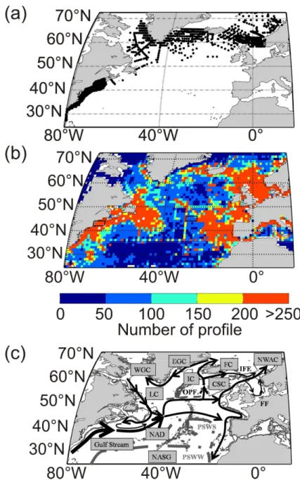
Biological data used in this study were located in the northern part of the North Atlantic Ocean and extended from 80 °W to 19.5 °E of longitude and 25.5 to 73 °N of latitude (Fig. 1a). Biological data came from different sources: the TASC programme (TransAtlantic Study on Calanus; http://tasc.imr.no) from 1995 to 1998 ; the U. S Georges Bank programme (http://globec.whoi.edu) from 1995 to 2000; the India survey (data provided by X. Irigoien) from 1971 to 1975; the Norwestlant programme (www.st.nmfs.noaa.gov/plankton; Heath et
3 4 5 6 7 8 9 10 11 12 13 14 15 16 17 18 19 20 21 22 23 24 25 26 27 28 29 30 31 32 33 34 35 36 37 38 39 40 41 42 43 44 45 46 47 48 49 50 51 52 53 54 55 56 57 58 59 60
For Peer Review
al. 2007) in 1963 ; the UK Marine Productivity project data held at BODC (www.bodc.ac.uk, Heath et al. 2007) from 2001 to 2002 ; the U. S Northeast continental shelf bongo survey (data provided by Jack Jossi) from 1977 to 2006; Labrador data in 1997, 2001 and 2002. Spatial distribution of the dataset is presented in Figure 1a and details of sampling methods are shown in Supplementary Table 1.
Chlorophyll-a data were gathered from the same surveys as the C. finmarchicus database and completed by downloaded data from the World Ocean Database (www.nodc.noaa.gov). Chlorophyll-a from the upper five meters were retained and integrated.
Physical data
Physical data utilised in this work were located in the North Atlantic Ocean, extending from 81.5 °W to 23.5 °E of longitude and 18.5 °N to 75 °N of latitude. Temperature and bathymetric data came from different high resolution profile sources. Some were provided by Conductivity-Temperature-Depth (CTD) data samples collected during the above biological cruises. Others came from the National Oceanic and Atmospheric Administration (NOAA, data provided by Maureen Taylor). Lastly, some data were downloaded from the World Ocean Database (www.nodc.noaa.gov) including Mechanical BathyThermograph (MBT), eXpendable BathyThermograph (XBT) and Profiling Floats (PFL) data. Data encompassed the period 1876-2008 (Fig. 1b). All profiles were taken from the surface to 500 m to focus on seasonal thermocline. The main surface currents and frontal structures of the region covered in this study are indicated in Fig. 1c.
Analyses
Identification of intensity and depth of the thermocline
2 3 4 5 6 7 8 9 10 11 12 13 14 15 16 17 18 19 20 21 22 23 24 25 26 27 28 29 30 31 32 33 34 35 36 37 38 39 40 41 42 43 44 45 46 47 48 49 50 51 52 53 54 55 56 57 58 59 60
For Peer Review
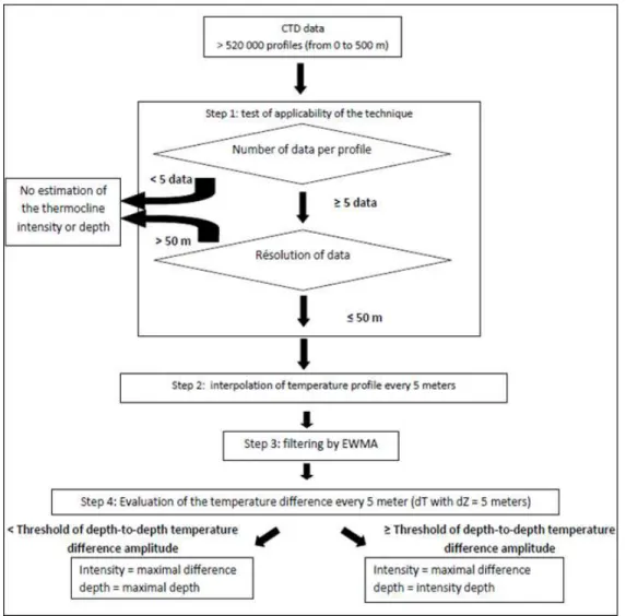
The techniques used to identify the depth and intensity of the thermocline have generally been empirical in the past. In this study, we designed a new procedure, which is summarised in Fig. 2. The procedure was divided into 4 steps:
Step 1: for each profile, two tests were performed before estimating the thermocline. The first
test measured the number of points in each profile. When the number of measures was strictly below 5 (threshold defined empirically in this paper), no estimation was made. The second test measured the resolution of the data. If the profile had a difference of more than 50 m and 20 m between successive depths (threshold defined empirically) in oceanic and neritic regions respectively, the information was considered too scarce and the estimation of depth and intensity of the thermocline was not calculated.
Step 2: the temperature of the profile was linearly interpolated for each interval of 5 m from
the original profile (in this study) (Lam, 1983). This interpolation was used to regulate the gap from one sample to another. No extrapolation was carried out here. Interpolation started at 2 meters to minimise the influence of the diurnal fluctuation of the water temperature and the noise related to the instrument in the first few meters (de Boyer Montégut et al., 2004). The procedure ended at the maximal depth of the profile (maximum 500 m). The interpolation technique was applied because the use of the weighted moving average in Step 3 needed equally spaced data.
Step 3: a filtering technique, named Exponentially Weighted Moving Average (EWMA)
(Montgomery, 1991), was applied on each temperature profile. This technique was chosen because it enables low or high persistent values to be better identified (Beaugrand and Ibanez, unpublished data). The technique is similar to the “cumulative sums”, another technique frequently used in statistical quality control (Ibañez et al., 1993). The technique was calculated by an iterative procedure and as follows:
1 0 (1 ). . + − − = z z A E E λ λ (1) 3 4 5 6 7 8 9 10 11 12 13 14 15 16 17 18 19 20 21 22 23 24 25 26 27 28 29 30 31 32 33 34 35 36 37 38 39 40 41 42 43 44 45 46 47 48 49 50 51 52 53 54 55 56 57 58 59 60
For Peer Review
Where Ez is the value of the moving average at depth z, Ez−1 is the value of the moving
average at depth z-1, A0 is the value of the initial dataset at depth z0 and λ is the filtering factor which is typically comprised between 0 and 1 and often fixed at 0.3 (Beaugrand and Ibanez, in preparation). The technique also enables a reduction of the noise inherent to this kind of data. The type of filtering is asymmetric contrary to most of the filtering methods (simple or weighted moving average, see Legendre & Legendre, 1998). This makes the method more sensitive to local variations.
Step 4: depth-to-depth absolute temperature difference d(T) was calculated every 5 meters as
follows: Za Zb T T T d( )= − (2)
Where TZb is the temperature at depth Zb and TZa is the temperature at depth Za., a and b ranging from 2 to 500m. The depth-to-depth temperature difference amplitude (i.e. the maximal minus the minimal difference in temperature calculated for each profile) was chosen to be the variable of the threshold method. This absolute difference amplitude marks a standardised increase or decrease of water temperature. In some cases, this variable can give the depth of the temperature inversions which occur at the base of barrier layers and in Polar Regions. When the depth-to-depth temperature difference amplitude was lower than a threshold (see Analysis 2), the thermocline intensity was fixed at the maximal difference of temperature and the thermocline depth was made equal to the maximal depth of the profile. In other cases, the thermocline intensity was fixed at the maximal value of d(T) and the depth of the thermocline was the depth at which the maximal value of d(T) was detected.
Before applying the procedure of identification of the depth and intensity of the thermocline (see previous analysis, step 4), it was important to select a threshold that allows
2 3 4 5 6 7 8 9 10 11 12 13 14 15 16 17 18 19 20 21 22 23 24 25 26 27 28 29 30 31 32 33 34 35 36 37 38 39 40 41 42 43 44 45 46 47 48 49 50 51 52 53 54 55 56 57 58 59 60
For Peer Review
the numerical procedure described in this paper to distinguish between a homogenous and a stratified water column. The selection of the threshold was done by performing 3 analyses.
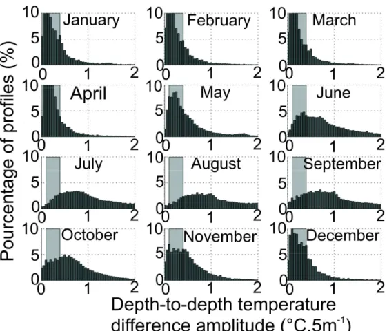
First, we examined monthly changes in the maximum depth–to-depth temperature difference (see Fig. 3) to evaluate the possible range of the different thresholds which could separate a homogenous from a stratified water column during a year, following descrptions in the literature (Longhurst, 1998; Pedlosky and Young, 1983). This analysis was conducted at a large-scale, covering the whole supratropical region of the North Atlantic and adjacent seas to consider the full range of conditions experienced by C. finmarchicus. We examined the interval of maximum annual variation (see Fig. 3) to temporarily select some thresholds for the next analysis in this interval.
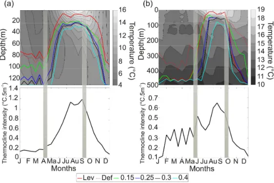
Second, we tested the new procedure against two types of averaged thermal profiles. Two regions were chosen to observe bi-monthly changes in the depth and intensity of the thermocline (see Fig. 1 and 4). The first station (see Fig 4a) was located between 42°N and 44°N and 66°W and 71°W and represented a neritic area of 132m mean depth. A total of 17,846 profiles were considered in this area. The second area (see Fig. 4b) was located between 44°N and 46°N and 25°W and 30°W. The region represented an oceanic area of 2620 meters mean depth. A total of 1,004 profiles were considered in this region. Temperature data were linearly interpolated every 5 meters for each profile from 2 meters to the maximal depth. A mean temperature was calculated for each depth and each two-week period. Mean bi-monthly depth and intensity of the thermocline were also calculated using the techniques of Levitus (1982) and Defant (1961). The Levitus (1982) method assesses the depth of the thermocline by calculating the differences between a reference point (here 0 m) and subsequent depths. A threshold of 0.5°C was selected by the author (Levitus, 1982). The Defant (1961) technique computes differences between successive depths with no prior transformation of the data. The threshold selected by the author was 0.015°C m-1 (Defant,
3 4 5 6 7 8 9 10 11 12 13 14 15 16 17 18 19 20 21 22 23 24 25 26 27 28 29 30 31 32 33 34 35 36 37 38 39 40 41 42 43 44 45 46 47 48 49 50 51 52 53 54 55 56 57 58 59 60
For Peer Review
1961). Our procedure was tested against these two techniques (see Analysis 1) but applied with different thresholds: 0.15, 0.25, 0.3, 0.4°C.5m-1. The threshold values were fixed per 5m because of the resolution of the profiles after interpolation, which corresponded to 0.03, 0.05, 0.06, 0.08°C.m-1. For both regions, the analysis of the intensity of thermocline was used to quantify the period of restratification and destratification. Restratification was considered as the first significant increase (i.e. increase of 5% from one point to the next) in the intensity of the thermocline. Destratification corresponds to the first significative decrease in the intensity of the thermocline (i.e. decrease of 5% from one point to the next). The Thresholds and methods were compared to the thermal profiles of the two regions.
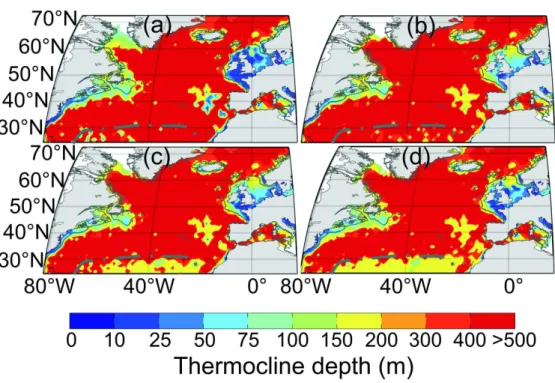
Third, both depth and intensity of the thermocline were mapped and the different thresholds examined at a macro-scale (Fig. 5). For each geographical cell of 1° of longitude and 1° of latitude, median depth and intensity of the thermocline were mapped after application of the techniques on each profile between 17.5 °E and 80.5 °W and between 30.5 and 72.5 °N. Spatial variation was computed using an isotropic variogram (Matheron, 1962) so as to compensate for gaps in the database, a kriging method based on the mgstat package of matlab (www.mgstat.sourceforge.net) was used. The spatial scale at which these parameters were mapped was selected to compare characteristic features of the whole supratropical region detected by other procedures (e.g. the transition zone between permanently and seasonally stratified regions at 40°N). Mapping was realised in spring (from April to June), summer (from July to September), autumn (from October to December) and winter (from January to March), using the method of Levitus (1982) and the technique proposed in this paper with different thresholds (see Analysis 1; see Fig.5). Our results were then compared to existing knowledge on North Atlantic circulation (Fig 1c.). The maps of the selected thresholds for the depth of the thermocline are represented in Figure 6 and the intensity of the thermocline in Figure 7. 2 3 4 5 6 7 8 9 10 11 12 13 14 15 16 17 18 19 20 21 22 23 24 25 26 27 28 29 30 31 32 33 34 35 36 37 38 39 40 41 42 43 44 45 46 47 48 49 50 51 52 53 54 55 56 57 58 59 60
For Peer Review
Relationships between the structure of the water column and Calanus finmarchicus
The objectives of these analyses were (1) to characterize the tolerance of each copepodite stage of C. finmarchicus to both the depth and the intensity of the thermocline and (2) to understand how the thermocline may affect the spatial distribution of the different copepodite stages.
Due to the variability in the sampling techniques among biological datasets (see Supplementary Table 1), a direct comparison based on abundance was likely to give biased results (Nichols and Thompson, 1991; Ohman, 2002). Therefore, we worked on relative frequency (Legendre and Legendre, 1998). To compute this index, the abundance data for each sampling sites and copepodite stages were integrated (BONGO and MOCNESS stratified dataset) on the whole water column sampled and converted into presence or absence. Then, for each geographical cell (spatial grid of 1° of longitude and latitude), month and year, the sum of the number of presences was divided by the total number of samples for each copepodite stage. Due to the likely overestimation or underestimation (mesh of 35-96 µm for early stages) of some specific copepodites by the different sampling techniques (Nichols and Thompson, 1991; Ohman, 2002), their potential influences were tested to estimate potential biases in the dataset. Relative presence was computed with and without all the different sampling techniques. No significant difference was observed between datasets, therefore the analyses presented in this article were performed with the whole database.
Physical observations (i.e. mean depth and intensity of the thermocline) were then integrated for each biological sample. Physical data were attributed to biological samples with the same month and year (at a temporal resolution of 15 days) and being at a maximum spatial distance of 0.2° of latitude or longitude. The first analysis characterised the tolerance of the species to the thermocline intensity and depth. The mean relative frequency of the
3 4 5 6 7 8 9 10 11 12 13 14 15 16 17 18 19 20 21 22 23 24 25 26 27 28 29 30 31 32 33 34 35 36 37 38 39 40 41 42 43 44 45 46 47 48 49 50 51 52 53 54 55 56 57 58 59 60
For Peer Review
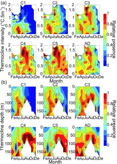
different stages of the species as a function of the intensity of the thermocline was assessed from 0 °C.5m-1 to 2 °C.5m-1 using a regular interval of 0.05°C.5m-1. A tolerance diagram was also built to examine the relative presence of the different stages of C. finmarchicus as a function of the depth of the thermocline from 0 m to 200 m by using a regular interval of 25 m. This procedure was applied for each every month and each copepodite stage (from stage 1 to adult) (see Fig. 8).
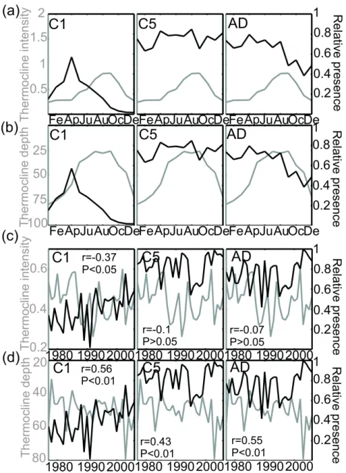
Secondly, correlations between the relative presence of C. finmarchicus and both the intensity and depth of the thermocline were calculated at the scale of the North Atlantic Ocean for the months between April and June (see Fig. 9). Prior to performing this analysis, the relative presence of the species was averaged for categories of 0.05°C.m-1 of thermocline intensity ranging from 0 to 1.5°C.5m-1 and for categories of 10m of depth between 0 and 200 m. Only intervals with an observation were considered when performing the linear regression. Third, an average of thermocline intensity and depth was calculated for the whole region where C. finmarchicus occurs at both monthly and year-to-year scales. The relative presence of C. finmarchicus was reported on the graphs to examine potential relationships between the species (copepodite stage 1, 5 and adults) and the mean characteristics of the thermocline (see Fig. 10). The objective of this analysis was therefore to study the relationships between the species and the thermocline by averaging the space and focussing on time at both seasonal and year-to-year scales.
Relationships between C. finmarchicus and environmental parameters
To understand how stratification affects the relative frequency of the species, the relation between thermocline (depth and intensity), surface chlorophyll-a and C. finmarchicus was investigated. Data on relative presence of C. finmarchicus were averaged for categories of chlorophyll-a of 0.075µg.l-1 between 0 and 4.2µg.l-1. Then, correlations were calculated
2 3 4 5 6 7 8 9 10 11 12 13 14 15 16 17 18 19 20 21 22 23 24 25 26 27 28 29 30 31 32 33 34 35 36 37 38 39 40 41 42 43 44 45 46 47 48 49 50 51 52 53 54 55 56 57 58 59 60
For Peer Review
between the relative presence of C. finmarchicus and the concentration of chlorophyll-a for all copepodite stages (see Fig. 11). Data of chlorophyll a were averaged for categories of 0.05°C.m-1 of thermocline intensity ranging from 0 to 1.5°C.5m-1 and for categories of 10m for the depth of the thermocline from 0 to 200 m in continental shelf regions and from 0 to 500 m in oceanic regions. Then, correlations were calculated between both the intensity and the depth of the thermocline and the chlorophyll-a concentration (see Fig. 12).
Results
Selection of a threshold to discriminate a homogeneous from a stratified water column
A fundamental step before running the technique for each thermal profile was to choose a relevant threshold to discriminate between a homogeneous and a stratified water column. This was done by performing three analyses. The first analysis used frequency histograms of the depth temperature difference amplitude (i.e. maximum depth-to-depth temperature difference) found in each profile and each month (Fig. 3). Between December and April when the water column was mainly homogeneous and June and September when the water column was mostly stratified, pronounced changes (maximal annual variation) were observed between 0.1°C.5m-1 and 0.4°C.5m-1 (Fig. 3). This analysis enabled the selection of potential thresholds between 0.1°C.5m-1 and 0.4°C.5m-1 to discriminate between a homogeneous and a stratified water column. Such a range of potential thresholds coincided with values commonly found in the literature (Thomson and Fine, 2003).
The second analysis tested our procedure with different thresholds in the range determined previously (see Fig. 3) against two other already published methods (Defant, 1961; Levitus, 1982) in a neritic (Fig. 4a) and an oceanic region (Fig. 4b). In the neritic region during the winter mixing period from December to April, the method of Defant and Levitus and our
3 4 5 6 7 8 9 10 11 12 13 14 15 16 17 18 19 20 21 22 23 24 25 26 27 28 29 30 31 32 33 34 35 36 37 38 39 40 41 42 43 44 45 46 47 48 49 50 51 52 53 54 55 56 57 58 59 60
For Peer Review
procedure based on a threshold of 0.15°C.5m-1 localised the depth of the thermocline shallower than with other thresholds (Fig. 4a). The restratification period was detected in April in the neritic region and at the end of May in the oceanic region with a significant increase in the slope of the depth of the thermocline (Fig 4). This period was well identified with all the techniques and thresholds except for the threshold of 0.4°C.5m-1 in the neritic region (Fig 4a). In the oceanic region (Fig. 4b), the methods of Levitus and Defant and our technique based on thresholds of 0.15°C.5m-1 localised the thermocline between April to May. When thresholds of 0.3°C.5m-1 and 0.4°C.5m-1 were used, the technique identified the establishment of the thermocline at the beginning of June. During the summer stratification (strong stratification between June and September), the methods of Levitus and Defant represented the depth of the thermocline shallower than our method. The destratification period detected in September for both regions was well detected with all the procedures with the notable exception of the technique of Levitus that localised the destratification in October. Among all the techniques and thresholds, the results indicated that our procedure based on a threshold of 0.25°C.5m-1 gave the closest match in term of depth. Furthermore, the intensity assessed from our technique with a threshold of 0.25°C.5m-1 gave a satisfactory summary of the structure of the water column (Fig. 4). Similar results were observed in the oceanic region (Fig. 4b). Here also, the threshold of 0.25°C.5m-1 gave the best compromise between a too conservative result (threshold of 0.4°C.5m-1) and too much sensitivity (Defant, followed by Levitus). In all cases, the procedure of Defant was too sensitive and was therefore excluded from the next analysis.
At a basin scale, the comparison of the Levitus technique with our method based on the thresholds 0.25, 0.30 and 0.40°C.5m-1 showed a good correspondence in the spatial changes in the depth of the thermocline (Fig. 5). However, some differences were observed at
2 3 4 5 6 7 8 9 10 11 12 13 14 15 16 17 18 19 20 21 22 23 24 25 26 27 28 29 30 31 32 33 34 35 36 37 38 39 40 41 42 43 44 45 46 47 48 49 50 51 52 53 54 55 56 57 58 59 60
For Peer Review
the boundary between permanently and seasonally stratified regions. The Levitus method did not clearly detect this well-known boundary. The new technique gave the best contrast between both permanently and seasonally stratified regions (PSWW: permanently stratified water in winter, Fig. 1c) when the smallest threshold was used. We therefore selected the threshold of 0.25°C.5m-1 in the next analyses.
Seasonal changes in the spatial distribution of the depth and the intensity of the thermocline
Seasonal variability in the spatial distribution of the depth and the intensity of the thermocline were examined in the North Atlantic sector using our procedure with a threshold of 0.25°C.5m-1 (Fig. 6 and Fig. 7). Mapping of seasonal changes in the depth of the thermocline clearly located the Subtropical Convergence (PSWW and PSWS, Fig 1c). This front separates the permanently stratified regions of the North Atlantic Subtropical Province from the seasonally stratified extratropical provinces of the Atlantic Westerly Winds Biome as it was termed by Longhurst (1998). In the north of the Subtropical Convergence, deep mixing occurred and in most regions (e.g. the Subarctic Gyre) winter mixing was greater than 500m in winter (Fig. 6). The meso-scale variability associated with the path of the Gulf Stream was particularly well detected in winter and the singularity of the South West European Basin clearly identified (Fig. 1b). A very interesting feature was the detection of the influence of the circulation around the Subarctic Gyre that increases the depth of the mixing in summer and autumn (Fig. 6c-d). The knowledge about the spatial distribution of C. finmarchicus (Heath et al., 2008; Helaouët and Beaugrand, 2007; Planque and Fromentin, 1996) and the present results suggest that the species is predominantly present in those
3 4 5 6 7 8 9 10 11 12 13 14 15 16 17 18 19 20 21 22 23 24 25 26 27 28 29 30 31 32 33 34 35 36 37 38 39 40 41 42 43 44 45 46 47 48 49 50 51 52 53 54 55 56 57 58 59 60
For Peer Review
oceanic regions characterised by deep winter mixing. This condition is important but sea surface temperature is another essential controlling factor (Helaouët and Beaugrand 2007).
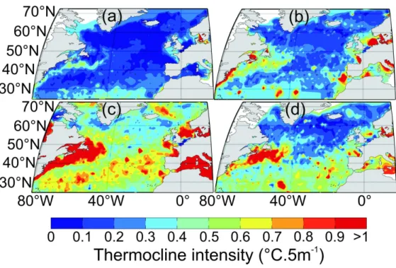
Mapping of the seasonal changes in the intensity of the thermocline showed the contrast between the winter and summer on the one hand and coastal and oceanic regions on the other hand (Fig. 7). In summer, the strongest thermoclines were detected over continental shelves and in the Mediterranean Sea where maximal intensity values were greater than 1°C.5m-1. In oceanic regions, intensity values oscillated between 0 and 0.3°C.5m-1 in temperate and in subpolar regions and 0.3 and 0.9°C.5m-1 in subtropical regions north of the Subtropical Convergence. Local hydro-dynamic features such as the Ligurian Front and the Flamborough front were also detected (Fig. 7 and Fig. 1b). The impact of surface currents on the intensity of the thermocline was clear. For example, weaker values were observed in the path of the Gulf Stream and around the Subarctic Gyre (Fig. 7).
Relationships between the structure of the water column and Calanus finmarchicus
To examine potential relationships between C. finmarchicus and the structure of the water column, we represented the relative frequency of the species as a function of the depth and the intensity of the thermocline (Fig. 8) for all the months from the copepodite stage 1 to the adult. The mapping of the relative frequency of the species as a function of the depth and intensity of the thermocline and the months revealed that young copepodite stages and especially copepodite stage 1 occurred in regions where the water column was not stratified (Fig. 8). Copepodite stage 1 individuals were less frequent in July. However, it was observed that a greater number of these stages were found in regions where the intensity of the thermocline was lower than 1 and the thermocline deeper than 50 m. Therefore, it is likely that copepodite stage 1 is less frequent during this month because it is not within its
2 3 4 5 6 7 8 9 10 11 12 13 14 15 16 17 18 19 20 21 22 23 24 25 26 27 28 29 30 31 32 33 34 35 36 37 38 39 40 41 42 43 44 45 46 47 48 49 50 51 52 53 54 55 56 57 58 59 60
For Peer Review
environmental niche (Fig. 8) (Helaouët & Beaugrand, 2007). When the individuals become older, stratification had much less influence and the species occurred in regions with both shallow and stronger thermocline. Adult stages seemed however to have a less wide range of habitats, than stage 5. The increase of tolerance to stratification occurring during the life cycle of the species is not consistent with the seasonal course of the thermocline.
To investigate more deeply the potential link between C. finmarchicus and the structure of the water column at a macroscale, we represented the mean relative frequency of the species as a function of the depth and the intensity of the thermocline (Fig. 9) for the months of maximum abundance. The results confirmed previous observations, showing a negative relationship between the species and the intensity of the thermocline. This relationship was especially high for copepodite stage 1. The negative relationship was not detected in May for Stage 5 (Fig. 9a). The examination of the sensitivity of the relationship, measured here by the strength of the correlation, indicated that adult stages were more sensitive to thermocline intensity than stage 5 but less than stage 1. The same sensitivity was found for all the stages when correlations were calculated between the relative presence of C. finmarchicus and the thermocline depth (Fig. 9b). The positive relationship between the relative presence of the species and the thermocline depth was however substantially lower for stage 5 in June.
An analysis was performed to investigate the temporal relationships between both thermocline depth and intensity and the relative presence of C. finmarchicus on both seasonal and year-to-year scales (Fig. 10). The analysis revealed that the youngest stages had their maximum relative presence just before the establishment of the thermocline (Fig. 10a). Stage 5 did not exhibit this relationship. On a year-to-year scale (period 1977-2005; n=28), the
3 4 5 6 7 8 9 10 11 12 13 14 15 16 17 18 19 20 21 22 23 24 25 26 27 28 29 30 31 32 33 34 35 36 37 38 39 40 41 42 43 44 45 46 47 48 49 50 51 52 53 54 55 56 57 58 59 60
For Peer Review
relationship with the thermocline (intensity and depth) was significantly highly negative for stage 1. No relationship was detected between thermocline intensity and the other stages (C5 and adult). Positive relationships between the relative presence of C. finmarchicus and the depth of the thermocline were also detected for all stages.
Relationships between C. finmarchicus and chlorophyll a concentration
Positive and significant relationships were detected between chlorophyll a and the relative presence of C. finmarchicus from stages 1 to 3. Then, the correlation became null for stage 4 and significantly negative for C5 and adults.
Relationships between the structure of the water column and chlorophyll a concentration
The relationship between water column stratification and chlorophyll-a was examined in both neritic (Fig. 12a) and oceanic (Fig. 12b) regions of the North Atlantic. Negative and significant relationships between chlorophyll-a and both intensity and depth of the thermocline were detected. Mean chlorophyll-a concentration was low in homogenous water (intensity of the thermocline < 0.25 °C.5m-1 and deep thermocline depth) and slightly increased when the intensity of the thermocline increased. Maximum chlorophyll-a concentration was located in the interval between 0.2 to 0.4 °C.5m-1 of intensity of the thermocline and between 40 and 60m of depth of the thermocline in the neritic area and between 100 and 230m in the oceanic area.
Discussion
The technique proposed to determine the depth and intensity of the thermocline is a gradient threshold method. This technique is usually considered to be a less consistent estimator of the thermocline than the “difference approach” (Thomson et al. 2003). However,
2 3 4 5 6 7 8 9 10 11 12 13 14 15 16 17 18 19 20 21 22 23 24 25 26 27 28 29 30 31 32 33 34 35 36 37 38 39 40 41 42 43 44 45 46 47 48 49 50 51 52 53 54 55 56 57 58 59 60
For Peer Review
because of problems related to the instruments used to sample or the presence of rapid environmental variation over a short depth range, temperature profiles are often piecewise-linear rather than smoothing varying (Brainerd and Gregg, 1995). The use of EWMA (Montgomery, 1991; Beaugrand and Ibanez, in preparation) gave us the possibility to obtain sharp gradient-resolved temperature profiles. EWMA was chosen because (1) the technique reduces the noise associated with temperature profiles and (2) in contrast to classical moving average methods, it is more sensitive to local variations (rapid temperature change), which is an important property for an accurate detection of the depth of the thermocline.
In this article, a thermocline is defined as the depth of maximal temperature change in the water column (maximal temperature gradient) and the concept is used as an indicator of water column stability. A prerequisite to the use of the technique was to define a threshold to separate a stratified from a homogenous water column. Three analyses were performed on different time and space scales and compared to two already existing methods (Defant, 1961; Levitus, 1982) with different possible thresholds. The technique, applied to both neritic and oceanic regions (Fig. 4), revealed that the Defant method and our technique based on a threshold of 0.15°C.5m-1 were too sensitive because they overrated the depth of the thermocline during winter and identified restratification too early. De Boyer Montégut et al. (2004) noticed that the method of Levitus (1982) did not accurately localise the initiation of stratification (Fig. 4). The analysis performed at a macroscale (Fig. 5) and the comparison with profiles (see Fig. 4) showed that the general pattern of thermocline depth was respected in comparison to the Levitus technique. The comparisons with the profiles (see Fig. 4 and 5) showed that the threshold of 0.25°C.m-1 gave the best results (see also the location of hydro-dynamic features in Fig 1c).
3 4 5 6 7 8 9 10 11 12 13 14 15 16 17 18 19 20 21 22 23 24 25 26 27 28 29 30 31 32 33 34 35 36 37 38 39 40 41 42 43 44 45 46 47 48 49 50 51 52 53 54 55 56 57 58 59 60
For Peer Review
The spatial distribution and seasonal variation of the thermocline appear to be in agreement with the knowledge on water column characteristics across the North Atlantic Ocean (Beaugrand et al., 2001; Sarmiento and Gruber, 2006; Sprintall and Tomczak, 1990; Tomczak and Godfrey, 2003). In Atlantic central gyres, the thermocline is deep and rapidly increases across frontal structures or main surface currents. Major currents such as the Gulf Stream, the Labrador Current or the European Continental Shelf Current are identified in our results and seasonal frontal structures (Oceanic Polar Front or Flamborough Front, Iceland-Faroe Front) are well represented (Fig. 6 and 7). The general pattern proposed in this study respects the location and the seasonality of these currents, and the quantification of the intensity of the thermocline provides additional information. A comparison between the monthly changes in these two descriptors (Fig. 4) and the description of the change in the characteristics of the thermocline by Longhurst (1998) are in agreement. Nevertheless, examination of seasonal changes in the depth of the thermocline shows that our technique described a deeper thermocline than previous studies (Levitus, 1982; Sprintall and Tomczak, 1990). Such a result can be explained either by the absence of consideration of the diurnal variation in the depth of thermocline in our analyses (de Boyer Montégut et al., 2004) or by the choice of the threshold of 0.25°C.m-1. Indeed, the greater the threshold, the less sensitive the method is regarding temperature change.
The present study used a new database on C. finmarchicus that can be complementary to the data collected by the Continuous Plankton Recorder (CPR) survey (Reid et al 2003). The present database is a compilation of several studies and surveys on the different copepodite stages of C. finmarchicus (supplementary Table 1.). This dataset has samples at different levels of the water column, information that cannot be obtained with CPR data (sampling at a constant depth of 7 m). Many authors have suggested an effect of stratification
2 3 4 5 6 7 8 9 10 11 12 13 14 15 16 17 18 19 20 21 22 23 24 25 26 27 28 29 30 31 32 33 34 35 36 37 38 39 40 41 42 43 44 45 46 47 48 49 50 51 52 53 54 55 56 57 58 59 60
For Peer Review
on the life cycle or the spatial distribution of different types of planktonic organisms (Planque and Fromentin, 1996; Rutherford et al., 1999). While Planque & Fromentin (1996) suspected an effect of stratification on the spatial distribution of Calanus finmarchicus and C. helgolandicus, Rutherford et al. (1999) provide evidence of a positive influence of this parameter on foraminifera diversity at a global scale. At a higher trophic level, mechanisms by which the column stability affects fish (tuna, anchovy, sardines) have been widely studied and are relatively well understood (Beare et al., 2004; Bertignac et al., 1998; Block et al., 1997; Brill et al., 1999; Lehodey et al., 1997). Beare and colleagues (2004) have revealed that water column stability could affect nutrition of small pelagic fish and thereby alter their growth and mortality or delay their biological development. For many Thunnidae, the thermocline affects their vertical and horizontal distributions (Bertignac et al., 1998; Block et al., 1997; Brill et al., 1999) and many reports suggest that a change in the depth of the thermocline (for example due to the Niño effect) might change the catchability of these species (Lehodey et al., 1997). Williams (1980a, 1980 b, 1985) speculated that, at the southern edge of the spatial distribution of C. finmarchicus, the vertical position of the thermocline may affect the abundance and the location of the species. Williams (1980b) found that the vertical position of C. finmarchicus was altered when the thermocline was stronger. This author suggested that this phenomenon allows the species to be separated from its congeneric species C. helgolandicus located shallower in the water column. The author speculated that this difference was related to the warmer thermal preference of C. helgolandicus. Subsequently, Williams (1985) supposed that this mechanism may also affect the nutrition strategy of the two species which compete for phytoplankton.
The link between stratification and C. finmarchicus was examined in different ways to detect and better understand how the species might be influenced by the characteristics of the
3 4 5 6 7 8 9 10 11 12 13 14 15 16 17 18 19 20 21 22 23 24 25 26 27 28 29 30 31 32 33 34 35 36 37 38 39 40 41 42 43 44 45 46 47 48 49 50 51 52 53 54 55 56 57 58 59 60
For Peer Review
water column stability. The macroecological study revealed a change in the environmental tolerance to stratification parameters occurring during the life cycle (Fig. 8). The results show that even if early life stages are found in different stratification conditions, they occurred more frequently (relative presence >0.5) in weakly stratified waters (0.1 and 0.3 C.5m-1 of intensity of thermocline and >50 m of depth of the thermocline) (Fig. 8 and 9). Older developmental stages were less sensitive to stratification (Fig. 8 and 9). Weak conditions of stratification were found before the establishment of the thermocline (March to May) when, in parallel, an increase in the relative presence of all copepodite stages was detected (Fig 10). The restratification period was characterised by an increase of the intensity of the thermocline (ranging between 0.2 and 0.5°C.m-) combined with a shallowing of the depth of the thermocline and exhibited an annual maximum of chlorophyll-a (Fig 12). Given the positive relationship between early stage and chlorophyll-a concentration (Fig 11) and the negative relationship between chlorophyll-a and the intensity of the thermocline (Fig. 12), it appears that the restratification period offers optimal environmental conditions for the species. Indeed, the results were in accordance with the observations made by Saumweber and Durbin (2006), who suggested that from March to May copepodite stages 5 emerged from diapause and became adults ready to spawn.
In the Arctic and Subarctic pelagic domain, sea surface temperature and chlorophyll-a concentration were driven by the incoming solar radiation and water stratification (Longhurst, 1998; Sverdrup, 1953). These two environmental parameters influence growth, nutrition, survival rate and therefore both temporal and spatial changes in the abundance of C. finmarchicus (Heath et al., 2008; Helaouët and Beaugrand, 2007). Furthermore, Cook et al. (2007) showed that early life stages were highly sensitive to both parameters suggesting that with low food concentration and high temperature conditions, young copepodites tended to disappear. Having said that, in winter and summer, the water column offers unsuitable
2 3 4 5 6 7 8 9 10 11 12 13 14 15 16 17 18 19 20 21 22 23 24 25 26 27 28 29 30 31 32 33 34 35 36 37 38 39 40 41 42 43 44 45 46 47 48 49 50 51 52 53 54 55 56 57 58 59 60
For Peer Review
environmental conditions for early life stages of C. finmarchicus. During these periods, survival rates of young copepodite stages may decrease due to food limitation in winter or too higher temperature in summer. It is only during the restratification period when the thermocline shallows, that epipelagic water contains both high food concentration (phytoplankton bloom) and an optimal temperature range for the reproduction and development of naupliar and young copepodite stages (Helaouët and Beaugrand, 2007; Cook et al., 2007). Based on our results and on previous findings (Hirst and Kiørboe, 2002; Ohman et al., 2004; Plourde et al., 2009), we suggest that stratification affects the occurrence of this subarctic species via both food concentration and temperature.
Change in global air/sea temperature in the Northern Hemisphere are assumed to move the boundaries between permanently and seasonally stratified waters polewards but also to reinforce the stratification in high latitudes according to Atmosphere-Ocean General Circulation models (Intergovernmental Panel on Climate Change, 2007; Sarmiento et al., 2004). In addition, the seasonal timing in the establishment of the thermocline is also expected to shift (Walther et al., 2002). These alterations could affect phytoplankton blooms and all associated trophic webs (Edwards and Richardson, 2004; Gowen et al., 1995). The ecological-niche and ecophysiological models of C. finmarchicus suggest changes in the spatial distribution of the species in the next decades (scenario A2 and B2) without including explicitly the influence of stratification. Our results suggest that the intensification of stratification or changes in its seasonal progression could alter the survival rate of early life stages of C. finmarchicus. As a consequence, this effect might limit the expected northward movement if the temperature continues to warm in the North Atlantic sector. The contraction of the species range could have a significant impact for ecosystem functioning by bottom-up
3 4 5 6 7 8 9 10 11 12 13 14 15 16 17 18 19 20 21 22 23 24 25 26 27 28 29 30 31 32 33 34 35 36 37 38 39 40 41 42 43 44 45 46 47 48 49 50 51 52 53 54 55 56 57 58 59 60
For Peer Review
or top-down propagation through the food web (Beaugrand et al. 2003) and have a potential impact on some biogeochemical cycles (Beaugrand 2009).
2 3 4 5 6 7 8 9 10 11 12 13 14 15 16 17 18 19 20 21 22 23 24 25 26 27 28 29 30 31 32 33 34 35 36 37 38 39 40 41 42 43 44 45 46 47 48 49 50 51 52 53 54 55 56 57 58 59 60
For Peer Review
Acknowledgements
The authors are grateful to all the people who helped to find or shared data: the programme TASC (Trans-Atlantic Study on Calanus; http://tasc.imr.no), the U. S Georges Bank programme (http://globec.whoi.edu); M. Heath for providing data from the UK Marine Productivity programme held at BODC (www.bodc.ac.uk), M. Taylor and J. Jossi for providing the U. S Northeast continental shelf bongo survey data, T. O’Brien and the web site Copepoda (www.st.nmfs.noaa.gov/plankton ), X. Irigoien and E. Head. Discussions with C. de Boyer-Montégut and F. Ibanez have improved our reflexion on the methodology used in this paper and the interpretation of the results. We are grateful to A.C Gandrillon for her help in the editing of the paper. Finally, the authors are grateful to the referees who helped to improve the study.
3 4 5 6 7 8 9 10 11 12 13 14 15 16 17 18 19 20 21 22 23 24 25 26 27 28 29 30 31 32 33 34 35 36 37 38 39 40 41 42 43 44 45 46 47 48 49 50 51 52 53 54 55 56 57 58 59 60
For Peer Review
Literature cited
Beare, B., Burns, F., Jones, E., Peach, K., Portilla, E., Greig, T., McKenzie, E., and Reid, D. (2004) An increase in the abundance of anchovies and sardines in the north-western North Sea since 1995. Global Change Biol., 10, 1209-1213.
Beare, D.J. and McKenzie, E. (1999) Temporal patterns in the surface abundance of C. finmarchicus and C. helgolandicus in the northern North Sea (1958-1996) inferred from the Continuous Plankton Recorder data. Mar Ecol Prog Ser, 190, 241-251. Beaugrand, G. (2009) Decadal changes in climate and ecosystems in the North Atlantic
Ocean and adjacent seas. Deep-Sea Res II. 56, 656-673.
Beaugrand, G. and Ibanez, F. (in preparation) Use of the Exponentially Weighted Moving Average (EWMA) to assess changes in the state of living systems.
Beaugrand, G., Ibañez, F., and Lindley, J.A. (2001) Geographical distribution and seasonal and diel changes of the diversity of calanoid copepods in the North Atlantic and North Sea. Mar. Ecol. Prog. Ser., 219, 205-219.
Beaugrand, G., Brander, K.M., Lindley, J.A., Souissi, S., and Reid, P.C. (2003) Plankton effect on cod recruitment in the North Sea. Nature, 426, 661-664.
Bertignac, M. , Lehodey, P., and Hampton, J. (1998) A spatial population dynamics simulation model of tropical tunas using a habitat index based on environmental parameters. Fish. Oceanogr., 7, 326-334.
Block, B., Keen, J., Castillo, B., Dewar, H., Freund, E., Marcinek, D., Brill, R., and Farwell, C. (1997) Environmental preferences of yellowfin tuna (Thunnus albacares) at the northern extent of its range. Mar. Biol., 130, 119-132.
Bopp, L., Aumont, O., Cadule, P., Alvain, S., and Gehlen, G. (2005) Response of diatoms distribution to global warming and potential implications: A global model study. Geophys. Res. Lett., 32, 4.
Brainerd, K. E. and Gregg, M. C. (1995) Surface mixed and mixing layer depths. Deep-Sea Res. Part I, 9, 1521-1543.
Brill, R., Block, B. , Boggs, C., Bigelow, K. , Freund, E. , and Marcinek, D. (1999) Horizontal movements and depth distribution of large adult yellowfin tuna (Thunnus albacares) near the Hawaiian Islands, recorded using ultrasonic telemetry: implications for the physiological ecology of pelagic fishes. Mar. Biol., 133, 395-408.
2 3 4 5 6 7 8 9 10 11 12 13 14 15 16 17 18 19 20 21 22 23 24 25 26 27 28 29 30 31 32 33 34 35 36 37 38 39 40 41 42 43 44 45 46 47 48 49 50 51 52 53 54 55 56 57 58 59 60
For Peer Review
de Boyer Montégut, C., Madec, G., Fischer, A. S., Lazar, A., and Ludicone, D. (2004) Mixed layer depth over the global ocean: An examination of profile data and a profile-based climatology. J. Geophys. Res. C, 109, C12003.
Defant, A. (1961). Physical Oceanography Vol. 1. Pergamon, New York, 729.
Dickson, R. and Brander, K. M. (1993) Effects of a changing windfield on cod stocks of the North Atlantic. Fish. Oceanogr., 2, 124 - 153.
Dietrich, G. (1964). Research in Geophysics : Oceanic polar front survey. Vol. 2. MIT Press, Cambridge, Massachusetts USA, 291.
Edwards, M. and Richardson, A.J. (2004) Impact of climate change on marine pelagic phenology and trophic mismatch. Nature, 430, 881-884.
Gowen, R. J., Stewart, B. M., Mills, D. K., and Elliott, P. (1995) Regional differences in stratification and its effect on phytoplankton production and biomass in the northwestern Irish Sea. J. Plankton Res., 17, 753-769.
Heath, M.R., Rasmussen, J., Ahmed, Y., , Allen, J., Anderson, C.I.H., Brierley, A.S., Brown, L., Bunker, A., Cook, K., Davidson, R., Fielding, S., Gurney, W.S.C., Harris, R., Hay, S., Henson, S., Hirst, A.G., Holliday, N.P., Ingvarsdottir, A., Irigoien, X., Lindeque, P., Mayor, D.J., Montagnes, D., Moffat, C., Pollard, R., Richards, S., Saunders, R.A., Sidey, J., Smerdon, G., Speirs, D., Walsham, P., Waniek, J., Webster, L., and Wilson, D. (2008) Spatial demography of Calanus finmarchicus in the Irminger Sea. Prog. Oceanogr. 76, 39-88.
Helaouët, P. and Beaugrand, G. (2007) Macroecology of Calanus finmarchicus and C. helgolandicus in the North Atlantic Ocean and adjacent seas. Mar. Ecol. Prog. Ser.,
345, 147-165.
Helaouët, P. and Beaugrand, G. (2009) Physiology, ecological niches and species distribution. Ecosystems, 12, 1235-1245.
Hirst, A. G. and Kiørboe, T. (2002) Mortality of marine planktonic copepods: global rates and patterns. Mar. Ecol. Prog. Ser., 230, 195-209.
Ibañez, F., Fromentin, J.M., and Castel, J. (1993) Application de la méthode des sommes cumulées à l'analyse des séries chronologiques en océanographie. Comptes Rendus de l'Académie des Sciences de Paris, Sciences de la Vie, 316, 745-748.
Intergovernmental Panel on Climate Change, Working Group I (2007). Climate change 2007: the physical science basis. Vol. 1. Cambridge University Press, Cambridge, 996.
3 4 5 6 7 8 9 10 11 12 13 14 15 16 17 18 19 20 21 22 23 24 25 26 27 28 29 30 31 32 33 34 35 36 37 38 39 40 41 42 43 44 45 46 47 48 49 50 51 52 53 54 55 56 57 58 59 60
For Peer Review
Kaiser, M. J., Attrill, M. J., Jennings, S., Thomas, D. N., Barnes, D. K. A., Brierley, A. S., Polunin, N. V. C., Raffaelli, D. G., and Williams, P. J. B. (2005). Marine ecology: processes, systems, and impacts. Vol. 1. Oxford University Press, U. S. A.,
Kara, A. B., Rochford, P. A., and Hurlburt, H. E. (2000) An optimal definition for ocean mixed layer depth. J. Geophys. Res. C, 105, 16803-16821.
Kara, A. B., Rochford, P. A., and Hurlburt, H. E. (2001), Naval Research Laboratory Mixed Layer Depth (NMLD) Climatologies, (7330-01-9995; Washington DC: Naval Research Laboratory).
Lam, N.S.N. (1983) Spatial interpolation methods: a review. Am Cartogr, 10, 129-49.
Lamb, P. J. (1984) On the mixed-layer climatology of the north and topical Atlantic. Dyn. Meteorol. Oceanol., 36, 292-305.
Legendre, P. and Legendre, L. (1998). Numerical Ecology. 2. Vol. 1. Elsevier Science B.V., The Netherlands, 853.
Lehodey, P., Bertignac, M., Hampton, J., Lewis, A., and Picaut, J. (1997) El Niño Southern Oscillation and tuna in the western Pacific. Nature, 389, 715-718.
Levitus, S. (1982). Climatological Atlas of the World Ocean. Vol. 1. United States Government Printing, Washington, DC,
Longhurst, A. (1998). Ecological Geography of the Sea. Academic Press, London, 390. Martin, P. J. (1985) Simulation of the mixed layer at OWS November and Papa with several
models. J. Geophys. Res. C, 90, 903-916.
Matheron, G. (1962). Traité de géostatistique appliquée. Vol. E.B.D.R.G.E. minières, Paris, 171.
Mauchline, J. (1998). The biology of calanoid copepods. Vol. Academic Press, San Diego, Monterey, G. I. and Levitus, S. (1997). Climatological cycle of mixed layer depth in the world
ocean. Vol. United States Government Printing, Washington, D.C 100.
Montgomery, D.C. (1991). Introduction to statistical quality control. 2. Vol. John Wiley and sons, Inc, New York, 674.
Nichols, J. H. and Thompson, A. B. (1991) Mesh selection of copepodite and nauplius stages of four calanoid copepod species. J. Plankton Res., 13, 661-671.
Obata, A., Ishizaka, J., and Endoh, M. (1996) Global verification of critical depth theory for phytoplankton bloom with climatological in situ temperature and satellite ocean color data. J. Geophys. Res. C, 101, 657-667.
2 3 4 5 6 7 8 9 10 11 12 13 14 15 16 17 18 19 20 21 22 23 24 25 26 27 28 29 30 31 32 33 34 35 36 37 38 39 40 41 42 43 44 45 46 47 48 49 50 51 52 53 54 55 56 57 58 59 60
For Peer Review
Ohman, M. D., Eiane, K., Durbin, E. G., Runge, J. A., and Hirche, H. J. (2004) A comparative study of Calanus finmarchicus mortality patterns at five localities in the North Atlantic. ICES J. Mar. Sci., 61, 687-697.
Ohman, M. D., Runge, J. A., Durbin, E. G., Field, D. B., Niehoff, B. (2002) On birth and death in the sea. Hydrobiologia, 480, 55-68.
Pedlosky, J. and Young, W. R. (1983) Ventilation, potential-vorticity homogenization and the structure of the ocean circulation. J. Phys. Oceanogr., 13, 2020-2037.
Pickard, G. L. and Emery, W. J. (1990). Descriptive Physical Oceanography: An Introduction 5. Vol. Pergamon, New York, 320.
Planque, B. and Fromentin, J.-M. (1996) Calanus and environment in the eastern North Atlantic. I. Spatial and temporal patterns of C. finmarchicus and C. helgolandicus. Mar. Ecol. Prog. Ser., 134, 111-118.
Plourde, S., Pepin, P., and Head, E. J. H. (2009) Long-term seasonal and spatial patterns in mortality and survival of Calanus finmarchicus across the Atlantic Zone Monitoring Programme region, Northwest Atlantic. ICES J. Mar. Sci.,
Price, J. F., Weller, R. A., and Pinkel, R. (1986) Diurnal cycling: Observations and models of the upper ocean response to diurnal heating, cooling, and wind mixing. J. Geophys. Res. C, 91, 8411-8427.
Rutherford, S., D'Hondt, S., and Prell, W. (1999) Environmental controls on the geographic distribution of zooplankton diversity. Nature, 400, 749-753.
Sarmiento, J.L. and Gruber, N. (2006). Ocean biogeochemical dynamics. Vol. Princeton University Press, Princeton and Oxford, 503.
Sarmiento, J.L., Slater, R., Barber, R., Bopp, L., Doney, S.C., Hirst, A.C., Kleypas, J., Matear, R., Mikolajewicz, U., Monfray, P., Soldatov, V., Spall, S.A., and Stouffer, R. (2004) Response of ocean ecosystems to climate warming. Global. Biogeochem. . Cycles, 18, 1-23.
Saumweber, W. J. and Durbin, E. G. (2006) Estimating potential diapause duration in Calanus finmarchicus. Deep-Sea Res. Part II, 53, 2597-2617.
Sprintall, J. and Tomczak, M. (1990), Salinity considerations in the oceanic surface mixed layer, in Ocean Sciences Institute Rep. (ed.), 36 ( Sydney: University of Sydney), 170. Sverdrup, H.U. (1953) On conditions for the vernal blooming of phytoplankton. ICES J. Mar.
Sci., 18, 287-295.
Thompson, Rory (1976) Climatological numerical models of the surface mixed layer of the ocean. J. Phys. Oceanogr., 6, 496-503.
3 4 5 6 7 8 9 10 11 12 13 14 15 16 17 18 19 20 21 22 23 24 25 26 27 28 29 30 31 32 33 34 35 36 37 38 39 40 41 42 43 44 45 46 47 48 49 50 51 52 53 54 55 56 57 58 59 60
For Peer Review
Thomson, R. E. and Fine, I. V. (2003) Estimating mixed layer depth from oceanic profile data. J. Atmos. Ocean. Technol., 20, 319-329.
Tomczak, M. and Godfrey, J.S. (2003). Regional Oceanography: an Introduction 2. Vol. 1. Daya Publishing House, Delhi, 390.
Wagner, R. G. (1996) Decadal-scale trends in mechanisms controlling meridional sea surface temperature gradients in the tropical Atlantic. J. Geophys. Res. C, 101, 683-694. Walther, G. R., Post, E., Convey, P., Menzel, A., Parmesan, C., Beebee, T. J. C., Fromentin,
J. M., Hoegh-Guldberg, O., and Bairlein, F. (2002) Ecological responses to recent climate change. Nature, 416, 389-395.
Weller, R. A. and Plueddemann, A. J. (1996) Observations of the vertical structure of the oceanic boundary layer. J. Geophys. Res. C, 101, 8789-8806.
Wijffels, S., Firing, E., and Bryden, H. (1994) Direct observations of the Ekman balance at 10°N in the Pacific. J. Phys. Oceanogr., 24, 1666-1679.
Williams, R. (1985) Vertical distribution of Calanus finmarchicus and C. helgolandicus in relation to the development of the seasonal thermocline in the Celtic Sea. Mar Biol 86, 145-149.
Williams, R. and Conway, D.V.P. (1980) Vertical distribution of Calanus finmarchicus and C. helgolandicus (Crustacea: Copepoda). Mar. Biol., 60, 57-61.
Williams, R. and Lindley, J. A. (1980a) Plankton of the Fladen Ground During FLEX 76 III. Vertical Distribution, Population Dynamics and Production of Calanus finmarchicus (Crustacea: Copepoda). Mar. Biol., 60, 47-56.
Williams, R. and Lindley, J.A. (1980b) Plankton of the Fladen Ground during FLEX 76 I. Spring development of the plankton community. Mar. Biol., 57, 73-78.
2 3 4 5 6 7 8 9 10 11 12 13 14 15 16 17 18 19 20 21 22 23 24 25 26 27 28 29 30 31 32 33 34 35 36 37 38 39 40 41 42 43 44 45 46 47 48 49 50 51 52 53 54 55 56 57 58 59 60
For Peer Review
3 4 5 6 7 8 9 10 11 12 13 14 15 16 17 18 19 20 21 22 23 24 25 26 27 28 29 30 31 32 33 34 35 36 37 38 39 40 41 42 43 44 45 46 47 48 49 50 51 52 53 54 55 56 57 58 59 60For Peer Review
Table Legends
Table 1. Selected equations for detecting the depth of the thermocline or mixed layer depth.
Methods are sorted chronologically. T is temperature and σθ is potential density. Z denotes the depth and ∆Z, ∆T and ∆σθ denote respectively the difference in depth and temperature and density.
Supplementary Table 1. Characteristics of all databases used in this study.
Figure Captions
Figure 1. (a) Spatial distribution of biological data (99 599 stations) .(b)Spatial distribution of
temperature profile data (1,005,619 profiles).(c) Schematic representation of main surface currents over the North Atlantic based on Beaugrand et al. (2001) , Sarmiento and Gruber (2006) , Longhurst (2007), Tomczak and Godfrey ( 2001); Currents. CSC: Continental Shelf Current; EGC: East Greenland Current; FC: Faroe Current; IC: Irminger Current; LC: Labrador Current; NAD: North Atlantic Drift Current; NWAC: Norwegian Atlantic Current; WGC: Western Greenland Current. Frontal structures; FF: Flamborough Front; IFF: Iceland-Faroe Front; OPF: Oceanic Polar Front. Other abbreviations. NASG : North Atlantic Sub-tropical gyre; PSWW: Permanently Stratified Water in Winter; PSWS: Permanently Stratified Water in summer;
Figure 2. Sketch diagram of the procedure allowing the estimation of the intensity and the
depth of the thermocline. The resolution, fixed by parameter x was equal to 5 meters in this study. Thresholds were fixed empirically.
2 3 4 5 6 7 8 9 10 11 12 13 14 15 16 17 18 19 20 21 22 23 24 25 26 27 28 29 30 31 32 33 34 35 36 37 38 39 40 41 42 43 44 45 46 47 48 49 50 51 52 53 54 55 56 57 58 59 60