Observed and projected Sea Surface Temperature seasonal changes in the Western English Channel from satellite data and CMIP5 multi-model ensemble

HAL Id: hal-01366664

https://hal.archives-ouvertes.fr/hal-01366664

Submitted on 15 Sep 2016

HAL is a multi-disciplinary open access

archive for the deposit and dissemination of

sci-entific research documents, whether they are

pub-lished or not. The documents may come from

teaching and research institutions in France or

abroad, or from public or private research centers.

L’archive ouverte pluridisciplinaire HAL, est

destinée au dépôt et à la diffusion de documents

scientifiques de niveau recherche, publiés ou non,

émanant des établissements d’enseignement et de

recherche français ou étrangers, des laboratoires

publics ou privés.

seasonal changes in the Western English Channel from

satellite data and CMIP5 multi-model ensemble

Blandine l’Hévéder, Sabrina Speich, Olivier Ragueneau, Francis Gohin,

Philippe Bryère

To cite this version:

Blandine l’Hévéder, Sabrina Speich, Olivier Ragueneau, Francis Gohin, Philippe Bryère. Observed

and projected Sea Surface Temperature seasonal changes in the Western English Channel from satellite

data and CMIP5 multi-model ensemble. International Journal of Climatology, Wiley, 2017, 37 (6),

pp.2831-2849. �10.1002/joc.4882�. �hal-01366664�

Peer Review Only

Observed and projected Sea Surface Temperature seasonal

changes in the Western English Channel from satellite data

and CMIP5 multi-model ensemble.

Journal: International Journal of Climatology Manuscript ID JOC-16-0247.R1

Wiley - Manuscript type: Research Article Date Submitted by the Author: n/a

Complete List of Authors: L’Hévéder, Blandine ; IPSL, LMD Speich, Sabrina; ENS, LMD

Gohin, Francis; IFREMER, DYNECO/PELAGOS Ragueneau, Olivier; IUEM, LEMAR

Bryere, Philippe; Groupe ACRI, 29

Keywords: SST, Climate change, Western English Channel, CMIP5, regional study

Peer Review Only

1

Observed and projected Sea Surface Temperature

Observed and projected Sea Surface Temperature

Observed and projected Sea Surface Temperature

Observed and projected Sea Surface Temperature

1

seasonal changes in the Western English Channel from

seasonal changes in the Western English Channel from

seasonal changes in the Western English Channel from

seasonal changes in the Western English Channel from

2

satellite data and CMIP5 multi

satellite data and CMIP5 multi

satellite data and CMIP5 multi

satellite data and CMIP5 multi-

--

-model ensemble.

model ensemble.

model ensemble.

model ensemble.

3

4

5

6

7

8

9

10

1 LEMAR, IUEM Technopôle Brest-Iroise, rue Dumont d'Urville, 29280 Plouzané, FRANCE

11

2 LMD, ENS, 24 rue Lhomond, 75231 Paris cedex 05, FRANCE

12

3 IFREMER/DYNECO/PELAGOS, Centre Ifremer de Brest, 29280 Plouzané, FRANCE

13

4 ACRI-HE, 40 Quai de la douane, 29200 Brest, FRANCE

14

15

16

17

Corresponding author: Blandine L'Hévéder, blandine.lheveder@lmd.jussieu.fr

18

tel: +33(0)6 62 53 32 37, fax: +33(0)1 43 36 83 92

Peer Review Only

2

Key words

20

SST, Climate change, Western English Channel, CMIP5, regional study.

21

Abstract

22

Seasonal Sea Surface Temperature (SST) changes in the Western English Channel have been

23

estimated for the previous decades from high-resolution satellite data. Coastal seas, well separated

24

from offshore waters by intense frontal structures, show colder SST by 1 to 2°C in summer. A

25

significant warming trend is observed in the autumn season. This positive trend is stronger offshore,

26

with an annual mean SST increase of 0.32°C/decade, but weaker in coastal waters (0.23°C/decade),

27

where strong vertical mixing induced by tides and winds acts to reduce surface warming. The

28

performance of an ensemble of CMIP5 climate model in simulating recent seasonal changes of SST in

29

the region is estimated. The median of CMIP5 models reproduces very well the observed SST mean

30

seasonal cycle in offshore waters but is less proficient in the coastal sector due to the coarse

31

resolution of the models and the absence of tidal forcing and related processes. In the Iroise Sea, a

32

region of intense biological activity located off the western tip of Brittany, the trend of the annual

33

mean SST is relatively well simulated, albeit somewhat underestimated (0.20°/decade) and evenly

34

distributed throughout the year. Here, the increase in annual mean SST in CMIP5 future scenarios

35

simulations ranges from 0.5°C (RCP2.6) to 2.5°C (RCP8.5) by year 2100, with a seasonal

36

modulation leading to a more intense warming in summer than in winter. This increase in SST may

37

strongly affect marine biology, particularly phytoplankton phenology, macro-algae biomass and benthic

38

fauna, including exploited shellfish, in the Western English Channel.

Peer Review Only

3

1. Introduction

40

Climate change will affect marine ecosystems in many different ways, through the alteration of the

41

physical environment, biogeochemical cycles, biodiversity, and hence ecosystem structure and

42

functioning (IPCC, 2014). The impact of climate change on biodiversity includes profound changes in

43

species distribution and abundance, leading to global extinction and alteration of ecosystem services

44

(Bellard et al., 2012). As a result of that, society, and in particular coastal communities, have to adapt

45

to these changes (Millennium Ecosystem Assessment, 2005). In order to move towards adaptation and

46

mitigation, there is a crucial need to improve the predictive capacity of models to depict future

47

changes in the physical environment, especially at local or regional scale. Among the most crucial

48

parameters to be studied, is sea surface temperature (SST). Temperature plays a fundamental role in

49

ocean processes (circulation, stratification), in controlling the thermodynamic and kinetic

50

characteristics of chemical and biogeochemical processes (degradation, dissolution, precipitation), in

51

controlling the spatial distribution, the metabolic rates and the life cycle of marine flora (Bissinger et

52

al., 2008; Chen, 2015) and fauna (Southward et al., 1995; Helmuth et al., 2006; Philippart et al, 2011;

53

Thomas et al., 2016). The region of interest for this study is the Western English Channel, an oceanic

54

region located off the western coasts of France, including the English Channel to the north, the Iroise

55

Sea in the central-west portion and the Bay of Biscay at the southern end (Figure 1). Inside, two

56

oceanic areas can be identified with different sea temperature sensitivities to global change. The first

57

one, composed of the southern Brittany and the offshore waters of the Western English Channel,

58

shows a seasonal stratification with frequent occurrences of a strong summer bloom of the harmful

59

dinoflagellate Karenia mikimotoi on the warm side of the seasonal front of SST (Vanhoutte-Brunier et

60

al., 2008, Hartmann et al., 2014). The second part of the region, essentially coastal but including also

61

the central EnglishChannel, is vertically well-mixed by tides (Gohin et al., 2015). In this area, a small

62

increase in the water temperature could have a dramatic effect on the kelp Laminaria digitata, which is

63

on the verge of local extinction due to the increase in sea temperature (Méléder et al., 2010, Raybaud

64

et al., 2013). This is also a biogeographic boundary zone and, in recent years, warm water species

Peer Review Only

4

have become much more common (Southward, 1980 ; Southward et al., 1995 ; Hawkins et al., 2003 ;

66

Southward et al., 2005 ; Hawkins et al., 2008 ; Smale et al., 2013). Ecological problems related to SST

67

change in the Western English Channel also include the alteration of nutrient delivery from land to

68

sea, development of invasive species such as Crepidula fornicata, Spartina sp., Crassostrea giga,

69

alteration of host-pathogen relationships and biological interactions (Poloczanska et al., 2008).

70

Biologists try to better understand the response of these populations to increasing SST (Altizer et al.,

71

2013).

72

There is a long history of research on the impacts of SST fluctuations on marine flora and fauna in

73

the Western English Channel (Southward et al., 2005). The studies have shown both warm

(1880-74

1890s, 1930-1950s) and cold periods (1960s to mid 1980s) before the recent period of rapid warming

75

driven by anthropogenic climate change. The time window studied here is the one of recent warming.

76

Over the last 30 years, the average surface temperature of the North Atlantic has risen (Rhein et al.,

77

2013). This trend is not uniform because of regional variability, and not all areas of the Northeast

78

Atlantic show the same long-term trends. However, the warming tendency of surface waters off the

79

coasts of Brittany is similar to the North Atlantic average temperature trend (Dye et al., 2013).In the

80

shallow seas of the Western English Channel, there is also substantial evidence of a warming over the

81

past decades inferred from satellite observations (Cannaby and Hüsrevoglu, 2009, Saulquin and Gohin,

82

2010, Dye et al., 2013) and from regional modelling studies (Michel et al., 2009, Holt et al., 2012). On

83

the wide northwest European continental shelf, global warming is modulated by mesoscale oceanic

84

processes, resulting in spatial patterns of SST that differ by their seasonal cycle, variability and trend.

85

To predict future climate change impacts on coastal ecosystems over the 21st century, an

86

assessment of the sea temperature evolution is necessary. In the framework of the IPCC's 5th report,

87

projections of future climate change have been made for several socio-economical scenarios with an

88

ensemble of Earth System Models (ESM). Nevertheless, ESMs invariably give a very poor

89

representation of the land-ocean interface and of the shelf seas. The reasons for this are twofold: first,

90

the resolution and, second, the representation of physical processes including the shelf sea barotropic

Peer Review Only

5

processes or the long gravity waves associated with tides and wind-generated coastally trapped waves

92

(Holt et al., 2009). Besides, there are few published regional model simulations with sufficient

93

resolution to include shelf sea processes (e.g. tidal mixing fronts and coastal currents) and of sufficient

94

duration to investigate how atmospheric and/or oceanic fluxes drive the interannual to decadal

95

variability. Focusing on regional models including our study region --that is the French Atlantic

96

shoreline and the English Channel-- only two simulations cover the recent past. Holt et al. (2012)

97

have modelled the temperature over the European continental shelf with the Atlantic Margin

98

configuration of POLCOMS at 12 km resolution over the period 1960-2002. Michel et al. (2009) have

99

analyzed the temperature variability in the Bay of Biscay through a simulation performed with a global

100

configuration of NEMO (resolution of ~20 km, but tides not simulated) for the period 1958-2004.

101

Besides that, a higher number of modelling studies have been undertaken to model the changes in

102

ocean properties in the North Sea (Schrum, 2001, Meyer et al., 2011, Hjøllo et al., 2009 ) and in the

103

Irish Sea (Young and Holt, 2007) over the previous decades.

104

Downscaling of climate change scenarios have also been performed over the European

105

continental shelf. Adlandsvik (2008) has compared a global climate simulation implemented with the

106

BCM model under the SRES-A1B scenario (IPCC, 2007) with the associated downscaled simulation

107

with ROMS over the North Sea at 8 km resolution. Later on, Friocourt et al. (2012) have used two

108

hydrographic models for the downscaling of the same scenario over the North Sea, but only for a

20-109

year period in the near future (2040s). Their study covers also the impacts on the phytoplankton

110

blooms using an ecological model. In the Irish Sea, Olbert et al. (2012) have downscaled the

SRES-111

A1B scenario using ECOMSED model at 2km resolution. Finally, regarding our region of interest, an

112

ocean simulation of the European continental shelf has been performed with the regional ocean model

113

POLCOMS (at 12 km resolution) nested in the ESM HadCM3 under the SRES-A1B scenario (Holt et

114

al., 2010). Only the latter study covers the French Atlantic shoreline and the English Channel. It is

115

therefore necessary to go further and to investigate the variety of climate models responses to future

116

climate change in this region. Following Hawkins and Sutton (2009), the dominant sources of

Peer Review Only

6

uncertainty for surface temperature prediction at regional scale are model and scenario uncertainties,

118

for time horizons of many decades or longer. To reduce model uncertainty, Foley (2010) has

119

demonstrated the efficiency of multi-model ensemble analysis.

120

The aim of this work is to evaluate the seasonal changes for SST in the Western English

121

Channel in the previous decades (1980-now) and up to the end of the 21st century. To take into

122

account the issues of uncertainty, we choose to analyze a multi-model ensemble of global climate

123

models from the Coupled Model Intercomparison Project Phase 5 (CMIP5; Taylor et al., 2012), for

124

three Representative Concentration Pathway (RCP) scenarios (IPCC, 2014). For the previous decades,

125

the warming trend detected in CMIP5 models is validated by that estimated from satellite data, in the

126

three seas around Brittany at the grid scale of the models (~100 km). Then, changes in the SST

127

seasonal cycle are assessed from the projections of CMIP5 models for future climate. The paper is

128

organized as follows. In Section 2, the data sets and methodology are described. In Section 3, an

129

overview of the changes in the SST seasonal cycle around Brittany over the last decades is presented.

130

Then, future changes are estimated for the Iroise Sea, region of special interest for its intense

131

biological activity. Section 4 addresses the expected impacts of the SST changes on the marine

132

ecosystems and concludes.

133

2. Data Sets and methodology

134

2.1 CMIP5 climate models

135

Daily SST fields have been retrieved from the Earth System Grid (ESG) data portal

136

(http://pcmdi9.llnl.gov/esgf-web-fe/) for 13 CMIP5 models (cf. Table 1). Most of them are European

137

models, in which the northern mid-latitude climate is likely to have been further validated. Only one

138

(typically the first) ensemble member of each model is used. The past analysis is based on the

139

historical simulation of the CMIP5 models for the period 1980-2005, and the future change on the

140

projections for three RCP scenarios (RCP2.6, 4.5 and 8.5; Moss et al., 2010) over the period

2006-141

2100. The historical simulations employ historical changes in the atmospheric composition reflecting

142

both anthropogenic and natural sources, and include time-evolving land cover information (Taylor et

Peer Review Only

7

al., 2012). Then, the peak-and-decline RCP2.6 scenario is designed to meet the 2°C global average

144

warming target compared to pre-industrial conditions by 2100 (van Vuuren et al., 2011a). Radiative

145

forcing in RCP4.5 peaks at about 4.5 W/m2 in year 2100 (Thomson et al., 2011). RCP8.5 assumes a

146

high rate of radiative forcing increase, peaking at 8.5 W/m2 in year 2100 (Riahi et al., 2011).

147

Figure 1 pictures the regional seas located off the coasts of French Brittany : the English

148

Channel, the Iroise Sea and the Bay of Biscay. Each of these seas has specific characteristics, linked

149

to local topography, continental geometry, hydrology, and will be analyzed separately. Most of CMIP5

150

oceanic models have a typical low spatial resolution, of about 110 km x 110 km at 48°N (see a typical

151

CMIP5 grid cell on Figure 1), so that the regional seas are modelled by only some grid cells and

152

shallow bathymetry is not well represented. The English Channel is not depicted in some models, nor

153

is it connected to the North Sea in others (see detailed characteristics of the different grid

154

topographies and geometries in Tab. 1). Tides and sub-mesoscale processes are not simulated but the

155

complete ocean-atmosphere system is modelled, including heat and energy exchanges between ocean

156

and atmosphere, essential to predict climate change.For each of the 13 CMIP5 ocean models, the grid

157

points localized in each of these seas are selected, and daily SST data are spatially averaged to

158

produce time series representative of the SST evolution in each sea.

159

2.2 Satellite observations and characteristic surface waters in Brittany's sea

160

A set of satellite data was used to validate the model-simulated SST around Brittany: the Ifremer

161

SST data derived from AVHRR/Pathfinder products interpolated by kriging (Saulquin and Gohin,

162

2010); the OSTIA data provided by the Met Office using the Operational SST and Sea Ice Analysis

163

(OSTIA) system described in Donlon et al. (2011); and the ODYSSEA data, also derived from

multi-164

sensor data set incorporating microwave instruments, provided by MyOcean (Autret and Piollé, 2011).

165

A daily time series for the period 1986-2013 of high-resolution SST satellite data was obtained by

166

concatenating Ifremer AVHRR -derived SST data for 1986-2009, OSTIA data for 2010 and ODYSSEA

167

data for 2011-2013. A comparison with an homogeneous time series covering the entire period,

168

stemming from global low-resolution GHRSST, showed that the inhomogeneity of the high-resolution

Peer Review Only

8

time series used here did not generate bias. The three sets of SST data were projected onto the same

170

regular grid --- 0.075° in longitude and 0.05° in latitude --- allowing a high spatial resolution of

171

about 5 km x 5 km.

172

Analyzing the Ifremer AVHRR-SST satellite data over 1986-2006, Saulquin and Gohin (2010)

173

have shown that the mean annual warming of the SST was not spatially uniform in the English Channel,

174

due to local physical and hydrodynamic oceanic processes. Indeed, fronts develop in summer and

175

autumn, delimiting at the surface a warm area --at the north west of the Ushant front-- from a cold

176

one, both differing also in their vertical structure. The area with a warm surface layer lies in thermally

177

stratified open waters, while cold surface water lies in tidally mixed coastal waters. Figure 1 shows a

178

snapshot of the SST on 18th June 2003, where sharp discontinuities in SST can be observed in the

179

middle of the English Channel as well as in Iroise Sea (Iroise front) and off Ushant (Ushant front), with

180

SST differences across the fronts of about 2°C. These fronts and their formation process have been

181

long and extensively studied (Pingree and Griffiths, 1978 ; Simpson et al., 1978 ; Mariette and Le

182

Cann, 1985 ; Le Boyer et al., 2009) and modelled (Muller et al., 2007 ; Cambon, 2008 ; Lazure et al.,

183

2009).

184

To take into account the spatial inhomogeneity of the SST in the seas surrounding Brittany, areas

185

with specific characteristics have been selected in each regional sea: « tidally mixed coastal waters »,

186

hereafter denoted by TiMCW and « thermally stratified open waters », ThSOW. They are represented

187

in Figure 1. In the Bay of Biscay, tides are weaker and mainly ThSOW are observed.

188

189

Above all, a comparison of the satellite data spatially averaged to the same spatial scale as CMIP5

190

models is essential, in order to smooth the sub-mesoscale variability present in the satellite data but

191

not simulated in the models. For each of the three seas, a time series representing the large scale

192

behaviour of the satellite SST has been computed as its average over ThSOW and TiMCW boxes.

193

2.3 Methodology

Peer Review Only

9

The end-to-end methodology applied to the Iroise Sea is the following. A set of indices is defined

195

to characterize the SST seasonal cycle. They are computed from daily CMIP5 models data and

high-196

resolution satellite data, spatially averaged to typical model grid scale. A « portrait diagram » of the

197

different models performances to simulate the climatologic present-day observed SST seasonal cycle is

198

shown, based on the indices. Over the last decades, trends in the indices are estimated in models and

199

satellite data, to evaluate the past changes in the SST seasonal cycle and test their simulation in the

200

models. Finally, future changes in the SST seasonal cycle are estimated from CMIP5 projections.

201

2.3.1 Indices for the SST seasonal cycle

202

In order to quantify the warming trend and the SST seasonal cycle change, indices are necessary.

203

For the atmosphere, the Expert Team on Climate Change Detection and Indices (ETCCDI) has defined

204

a set of climate indices that provide a comprehensive overview of temperature and precipitation

205

statistics focusing particularly on extreme aspects (Karl and Easterling, 1999, Klein Tank et al., 2009).

206

Multivariate Oceanic and Climatic Index (MOCI) have also been derived from a combination of global

207

and regional climate indices to evaluate the impact of oceano-climatic changes on marine ecosystems

208

in the Bay of Biscay (Hemery et al., 2008). So far, no set of indices has been developed for

oceanic-209

only climatic characteristics.

210

We propose a set of 13 indices (defined in Table 2) to characterize the SST seasonal cycle. To

211

compute these indices, daily data have been used to capture the most comprehensive signal. The

212

time-averaged indices, I1 and I10 to I13, are directly computed from the daily time series. To estimate

213

the indices I2 to I9, corresponding to the extremes (minimum, maximum) and time course (dates of

214

minimum and maximum annual temperature, of spring and autumn onset) of the seasonal cycle,

215

methodologies commonly applied to characterize the seasonal cycle of the temperature (Wyrtki, 1965,

216

Eliseev and Mokhov, 2003, Saulquin and Gohin, 2010) have been used. Details on the computation are

217

given in Table 2.

218

Peer Review Only

10

2.3.2 Trend estimate

220

To quantify the recent SST changes, linear trends in the SST monthly mean time series (Fig. 4)

221

and in the indices time series (Figs. 5 to 7) were computed using a « Kendall's tau based slope

222

estimator » developed by Wang and Swail (2001). This estimator is robust to the effect of outliers in

223

the series and an iterative procedure prevents the Kendall test result from being affected by serial

224

correlation of the series. This method has been widely used to compute trends in hydrometeorological

225

series (e.g., Wang and Swail, 2001, Zhang et al., 2000) and taken up to estimate trends in climate

226

extreme indices time series by Zhang et al. (2005). Throughout the paper, we only show trends

227

considered as significant, taking a threshold level of 95%.

228

2.3.3 Model performance metrics

229

Given the large number of indices and models analyzed in this study, we have used a metric based

230

approach to assess model performance, based on the estimation of « model relative error » of model

231

climatologies (Gleckler et al., 2008) and adapted from Sillmann et al. (2013) application to climate

232

extremes indices. This provides a synthetic overview of each model performance relative to the others

233

for various indices characterizing the mean SST seasonal cycle under present-day climate.

234

The mean present-day SST seasonal cycle in CMIP5 models is assessed in the Iroise Sea, with

235

respect to satellite observations over ThSOW and TiMCW (defined in Section 2.3.1). The indices are

236

estimated at an annual frequency, as they characterize a feature of the annual cycle. For each index,

237

we consider the climatology of its yearly time series over the common period between observations and

238

models -- 1986-2004 --, at the model grid scale for models and averaged over ThSOW and TiMCW

239

areas for satellite data. The climatologies are noted Ix for the model X and Iy for the satellite

240

observations. The absolute value of the difference between models and observations climatologies is

241

noted Exy=|Ix - Iy|.

242

For each model X, the « model relative error » E'xy is then derived from the collection of

model-243

observation differences Exy for all models as

Peer Review Only

11

E'xy=EXY− Em E_m

245

with Em the median of the model-observation differences Exy for all models.

246

E’xy provides an indication of the performance of the model X relative to the multi-model

247

ensemble, with respect to satellite observations over an area in the Iroise sea. The median Em

248

represents typical model performance in the multi-model ensemble. E'xy values for all models and all

249

indices obtained for both areas of the Iroise sea are summarized in a “portrait” diagram (Figure 3),

250

discussed in Section 3.1.2.

251

3. Results

252

3.1 SST mean seasonal cycle in present-day climate

253

3.1.1 SST mean seasonal cycle in satellite observations and CMIP5 multi-model ensemble

254

The SST mean seasonal cycle in satellite data and in CMIP5 historical simulations has been

255

evaluated for each of the three seas around Brittany (Figure 2). It is computed over the period

1980-256

2005 for CMIP5 models and 1986-2013 for satellite data.

257

In the observations, as expected, the SST mean seasonal cycles in TiMCW and ThSOW differ in

258

summer and autumn. Due to the strong vertical mixing by tidal currents in coastal areas that prevents

259

the seasonal thermocline from establishing in summer (Pingree and Griffiths, 1978, Mariette and Le

260

Cann, 1985, Cambon, 2008), summer SSTs are colder in TiMCW than in ThSOW, with across front

261

differences of about 1°C in the English Channel to 2°C in the Iroise Sea. Surface ThSOW cool

262

earlier and faster in autumn, at the time when the seasonal thermocline disappears. In the TiMCW of

263

Iroise Sea and English Channel, the mean SST seasonal cycles of satellite data are in good agreement

264

with in situ-data from SOMLIT-Brest (at the outlet of the Bay of Brest) and SOMLIT-Astan (at the

265

outlet of the Bay of Morlay) (Tréguer et al., 2014).

266

In the three seas, the observed SST mean seasonal cycle in ThSOW is well simulated by the

267

median of CMIP5 models. Considering the low-resolution of climate models used here, it is important

Peer Review Only

12

to emphasize the absence of bias, distortion or shift in the median SST seasonal cycle of CMIP models,

269

especially in the Iroise Sea. In summer, we notice a higher dispersion between model estimates, with an

270

interquartile model spread ranging from 1.5°C in the Iroise Sea to 2°C in the English Channel. Each

271

model taken individually presents a bias, but if we consider CMIP5 models simulations as an ensemble

272

of climate simulations, the median of the ensemble represents well the observed SST mean seasonal

273

cycle. However, a few differences to the observations can be noted. In the Bay of Biscay, summer SST

274

are too warm by 1°C. In the English Channel, winter SST are too cold by 1°C. Finally, the

275

characteristics of TiMCW --colder summer SST-- are not simulated in CMIP5 models. This is due to

276

the absence of simulation of sub-mesoscale processes and tides in global models, dominant factors for

277

the SST in TiMCW. In ThSOW, processes of air-sea interactions predomines for the SST estimate

278

(Esnaola et al., 2012). The latter are relatively well simulated in CMIP5 ocean-atmosphere coupled

279

models, even if air-sea processes associated with sub-mesoscale oceanic structures have been

280

demonstrated to increase the heat and energy budget of the ocean surface waters (Hogg et al., 2009,

281

Chelton and Xie, 2010).

282

3.1.2 Models performance inter-comparison for the Iroise Sea

283

An inter-comparison of the different CMIP5 models performance in the Iroise Sea, using the

284

metrics described in Section 2.3.3, is shown on the portrait diagram (Figure 3). It represents the

285

relative magnitude of the « model relative error » for each index (columns) and for each model (rows).

286

The magnitudes of the « model relative errors » are colour-coded, with colder (resp. warmer) colors

287

corresponding to E'xy<0 (resp. E'xy>0) for models getting a better (resp. poorer) performance than

288

others on average. In the first two rows, the performance of the « mean » and « median » of the

multi-289

model ensemble is also displayed.

290

In the portrait diagram, the mean and median of the CMIP5 multi-model ensemble get the better

291

performance in representing the observed SST. This result is consistent with the conclusions of

292

Gleckler et al. (2008), Sillmann et al. (2013) and other multi-model studies. Indeed, some of the

293

systematic bias in each of the individual models are canceled out in the multi-model mean or median.

Peer Review Only

13

In ThSOW, the mean and median model index climatologies are really close to the observations, but

295

less in TiMCW, thereby confirming the results and analysis of Section 3.1.1. Therefore, in the

296

following, we focus on the evaluation of the models in ThSOW, more relevant. The models that

297

better simulate the mean present-day SST seasonal cycle in the Iroise Sea are CNRM, ICHEC,

298

HadCM3, MPI-MR and IPSL-MR. ICHEC, MPI-MR and CNRM have in common a higher ocean

299

resolution and a more realistic topography and coastline geometry of the region of study than other

300

models of the study; IPSL-MR, ICHEC and CNRM an higher atmospheric resolution. Regarding

301

HadCM3, its good performance compared to HadGEM2-CC and HadGEM2-ES (the new generation of

302

climate models of the MetOffice) is surprising also because the horizontal resolution has been refined

303

in the recent ocean and atmosphere model versions. In the literature, Gordon et al. (2000) have

304

demonstrated the very good skill of HadCM3 to simulate the SST with no flux adjustments, which was

305

very novative at this time. By contrast, HadGEM2 (Collins et al., 2011) includes improvement

306

designed to address specific systematic bias encountered in HadGEM1, namely Northern Hemisphere

307

continental temperature biases, which may impact SST in the region of study. This result highlights the

308

complexity of climate modelling in the fact that the realism of the simulations is not guaranteed to be

309

improved by increasing the model resolution.

310

3.2 Change of SST seasonal cycle in the previous decades

311

3.2.1 Overview of Western English Channel

312

The observed and modelled changes of the SST seasonal cycle in the last 30 years in the Western

313

English Channel are illustrated in Figure 4. Time series for 1980-2013 of monthly mean SST in the

314

satellite data (in ThSOW and in TiMCW) and in the CMIP5 models are produced for each of the seas

315

located around Brittany. For each time series representing the evolution of the SST in a particular

316

month, a monthly trend is shown if significant.

317

In the observations, a warming trend is visible in the last 30 years, concentrated during the

318

autumn season. This autumn trend is present in both ThSOW and TiMCW. It is stronger in ThSOW,

319

and reaches the maximum value of about 0.6°C/decade --- which gives a SST increase of 1.8°C in

Peer Review Only

14

30 years --- in the Iroise Sea and in the Bay of Biscay. In spring, in ThSOW, we note also a

321

significant trend of about +0.3°C/decade, this trend being more pronounced in the Iroise Sea. In

322

TiMCW, the entire water column has to be warmed, which leads to a lower ocean surface warming. In

323

summer, no significant trend can be detected, probably because of the higher interannual variability

324

during that season.

325

In CMIP5 models historical simulations, the observed warming trend is simulated. However, in the

326

Iroise Sea and in the English Channel, its seasonal distribution differs from the observed one. The

327

warming trend is found all over the year, except during summer, with smaller values of about

328

0.25°C/decade. In global models, the ocean surface warming trend seems more linearly linked to the

329

greenhouse gases radiative forcing, because of the poor simulation of continental shelf processes. As

330

pointed out by Holt et al. (2014) in their review paper, it is not just an issue of resolution: a suite of

331

specific dynamic processes act in regional seas, which along with their particular geographic setting act

332

to shape the climatic impacts and lead to responses that may be diff erent from the wider global ocean.

333

Indeed, Adlandsvik (2008), in a marine downscaling experiment of the SRES-A1B scenario over the

334

North Sea, has demonstrated that downscaling strengthen the surface ocean warming. The regional

335

model has a more realistic shelf sea stratification, and most of the warming can be trapped in the

336

surface mixed layer during the summer season, resulting in a better seasonal distribution. In our study,

337

we highlight the need to refine in the same way the spatial resolution and to model tides in the

338

Western English Channel.

339

On the other end, the Bay of Biscay has smaller tides so that the oceanic characteristics are

340

better simulated in climate models. Accordingly, the modelled warming trend seasonal distribution is

341

closer to that of satellite observations, albeit half.

342

3.2.2 Trends of SST seasonal cycle indices in the Iroise Sea

343

To quantify changes in the SST seasonal cycle in the Iroise Sea in previous decades, the indices

344

time series are shown in Figures 5 to 7, for the satellite observations averaged over the Iroise Sea,

345

over the ThSOW and TiMCW areas, and for the median of the 13 CMIP5 simulations, with their

Peer Review Only

15

interquartile range. In the left column, the absolute values of the indices are presented. The SST gap

347

between ThSOW and TiMCW in the Iroise Sea is highlighted, in particular in summer when the

348

difference between the annual maxima reaches 2.5°C. Time series of ThSOW and TiMCW are highly

349

correlated, pointing out the driving role of atmospheric surface forcing.

350

In the right column are shown the index anomalies relative to each index time-mean over

1986-351

2005, this being the common period between observations and models. For the multi-model ensemble,

352

anomalies are first calculated separately for each model, by removing the index time-mean of the

353

model simulation, and then the median of the models anomalies is computed. That way, the bias

354

between the different data sets is eliminated and clearer trends emerge in the CMIP5 multi-model

355

ensemble. For the models, we note that trends of index absolute values and anomalies differ often by

356

15 to 30%. Trends of anomalies, not affected by the bias between the models and thus more

357

representative of the variability, are discussed.

358

The annual mean of the SST has a significant warming trend in observations and models (Fig. 5). It

359

is slightly underestimated in models (+0.2°C/decade) compared to the observations

360

(+0.27°C/decade). In the observations, it is larger in the ThSOW (+0.32°C/decade) than in the

361

TiMCW (+0.23°C/decade). These trends are in the range of previous estimates for the same period

362

in the region, that is [+0.2°C/decade +0.5°C/decade] for observed SST (Cannaby and Hüsrevoglu,

363

2009, Michel et al., 2009, Smyth et al., 2010, Saulquin and Gohin, 2010, Holt et al., 2012) and

364

[+0.175°C/decade +0.3°C/decade] for modelled SST (Michel et al., 2009, Holt et al., 2012). The

365

underestimation of the SST trend in models compared to satellite data has also been observed by

366

Michel et al. (2009) in a regional modelling study of the Bay of Biscay, in spite of the higher resolution

367

of their simulation (about 20 km). Their SST trend is of +0.22°C/decade in the model versus

368

+0.37°C/decade in satellite data, over a domain ranging up to 15°W into the open ocean.

369

In the observations, the SST trend is concentrated in the autumn season (+ 0.41°C/decade). The

370

other indices do not show significant trend. In ThSOW, the date of the autumn onset is also delayed

371

by 4 day/decade, certainly related to the strong autumn temperature increase of +0.48°C/decade.

Peer Review Only

16

The warming is there also fairly strong in spring (+0.3°C/decade).

373

CMIP5 models show a significant increase of the annual maximum (+0.31°C/decade), higher than

374

that of the annual minimum (+0.19°C/decade), resulting in an increase of the annual SST amplitude.

375

The annual maximum increase is not detected in the time series of indice I3 absolute value (Fig. 5, left

376

column) because of the large inter-model dispersion for summer temperatures. There is no significant

377

or a too weak trend in the time series of indices I5 to I8 (Fig. 6), that characterize a possible seasonal

378

shift. Indeed, models present a constant warming over all seasons of about +0.21°C/decade, with no

379

significant seasonal shift.

380

3.2.3 Natural climate variability versus anthropogenic climate change

381

In Western European marine systems, it is important to take into account the combined effects of

382

natural climate variability and anthropogenic climate change to conclude on warming trends related to

383

climate change. Nevertheless, whereas it is clear that there is a significant multidecadal pattern in the

384

SST, there is still much uncertainty about how to determine the relative contribution of these two

385

factors to the recent observed warming (Knight et al., 2005, Cannaby and Hüsrevoğlu, 2009, Swanson

386

et al., 2009, Ting et al., 2009). In our study, trends are computed over a relatively short period (28

387

years in the observations) compared to the 60 years cycle of the Atlantic Multi-decadal Oscillation

388

(AMO) natural variability pattern observed over the North Atlantic (Knight et al., 2005). The latter is

389

characterized by a SST increase over 1980-2007, followed by a decrease up to 2013. Cannaby and

390

Hüsrevoglu (2009) have shown that under the AMO warming phase, the AMO variability is responsible

391

for 50% of the warming trend on the northwestern European coast. If a too short period is considered,

392

the trend should rather be attributable to AMO natural variability than to anthropogenic climate

393

change, as in Tréguer et al. (2014), wherein a not really significant slightly negative trend was

394

estimated over the period 1998-2012 in the coastal area of Iroise Sea. Saulquin and Gohin (2010),

395

using the same AVHRR-SST satellite data as this study over the period 1986-2006, found identical

396

spatial distribution of the SST trend with slightly larger values of +0.4°C/decade in TiMCW to

397

+0.5°C/decade in ThSOW. As the period we consider extends up to 2013 and thus contains both a

Peer Review Only

17

warming and a cooling phase of the AMO natural variability cycle, it explains the slight trend

399

overestimation in Saulquin and Gohin (2010) and gives more confidence to the trend values of our

400

study as being for a major part attributable to anthopogenic climate change.

401

3.2.4 Conclusion on SST trends in the Iroise Sea over the previous decades

402

In the off-shore area of the Iroise Sea, the observed mean seasonal cycle of the SST is well

403

simulated by the CMIP5 multi-model ensemble (Section 3.1). Over the last 30 years, the annual mean

404

warming is slightly underestimated in models, with an evenly distribution throughout the year and no

405

seasonal shift; whereas observations show a seasonal shift due to a strong autumn warming, less

406

noticeable in the rest of the year (Section 3.2).

407

Despite these slight differences, it is appropriate to use the CMIP5 multi-model median derived

408

from the 5th IPCC future scenarios projections to evaluate the future SST evolution in the Iroise Sea.

409

3.3 Future scenarios

410

In this Section, future changes of SST seasonal cycle in the off-shore area of the Iroise Sea

411

are estimated from the projections carried out in CMIP5 for the scenarios established in the 5th IPCC

412

report (IPCC, 2014). Figure 8 (resp. 9) shows time series of indices I1 to I4 (resp. seasonal indices I10

413

to I13) for the 13 CMIP5 multi-model ensemble median, over 1980-2004 for historical simulations and

414

2005-2100 for the scenarios RCP2.6, RCP4.5 and RCP8.5 (described in Section 2.1). Anomalies of

415

indices relative to the time-mean over 1986-2004 are plotted, as in the left column of Figures 5 to 7.

416

Fits to second order polynomial functions are superimposed.

417

We note an increase of the SST annual mean of 0.5°C for the RCP2.6 scenario to 2.5°C

418

for the RCP8.5 one in year 2100. The uncertainty linked to the scenarios, of about 1.5°C for the

419

winter minimum, is half that of the summer maximum. In the scenario RCP2.6, the annual mean and

420

summer SST increase up to around 2060 and then decline. It is consistent with the radiative forcing

421

evolution (Van Vuuren et al., 2011), but with a time-lag of 10 to 20 years. In year 2100, seasonal

422

means converge to a constant warming all year round of +0.5°C. In the scenario RCP4.5, we note an

Peer Review Only

18

increase followed by a stabilization of the SST around year 2080, again with a time-lag of 10 to 20

424

years with respect to the imposed radiative forcing. At year 2100, the annual mean is forecast to reach

425

+1°C with a seasonal range of [+0.8°C +1.5°C]. In the scenario RCP8.5, a high rate of surface

426

temperature increase follows the radiative forcing, reaching +2.5°C for the annual mean with a

427

seasonal range of [+2°C +3.5°C] in year 2100.

428

For all scenarios, the warming is more moderate in winter-spring and stronger in

summer-429

autumn (Fig. 9). The warming difference between winter and summer is also highlighted in regional

430

downscaled projections over the North Sea (Adlandsvik, 2008), the western European continental shelf

431

(Holt et al., 2010) and the Irish Sea (Olbert et al., 2012). Holt et al. (2010), analyzing the SST and

432

hydrography changes by the end of the century in a downscaling study including our study region,

433

associated the SST changes to increasing summer stratification. From a regional perspective, a

434

comparison between our results and that of the latter study is interesting, although somewhat tricky

435

because different scenarios are simulated. In scenario SRES-A1B, Holt et al. (2010) simulate an

436

increase of the Iroise Sea SST of about +2.5°C in winter to +3.5°C in autumn. The scenario

SRES-437

A1B is close to the scenario RCP6.0, with a radiative forcing increase between scenarios RCP4.5 and

438

RCP8.5. In our study, the range between scenarios RCP4.5 and RCP8.5 gives an increase of [+0.8°C

439

+2°C] in winter to [+1.3°C +3°C] in summer. Thus, the warming on the shelf seems

440

underestimated in global climate models, especially in summer-autumn, due to a poor simulation of

441

physical and hydrographical processes specific to the oceanic shelves in Brittany.

442

To go further in the analysis, we now focus on future changes in SST interannual variability

443

and extremes. Indeed, climate change is likely to be associated with an increase of the occurence of

444

extreme events (IPCC, 2014), linked to a modification of the statistical distribution of the climate

445

variables. Changes in the shape of the probability distribution of SST may contribute as much to

446

changes in extremes as a shift of mean temperatures (Schaeffer et al., 2005). To evaluate the changes

447

in mean seasonal SST extremes, the probability distribution functions (PDF) of the winter and summer

448

mean SST in CMIP5 multi-model ensemble are represented in Figure 10 for the present-day climate

Peer Review Only

19

(1986-04), the near-future (2031-50) and the far-future (2081-2100) climates. Changes in inter-model

450

variability are negligible compared to changes in interannual variability (not shown). In the near-future,

451

a similar increase of SST characteristics (mean and variance) is simulated in all three scenarios for both

452

seasons. In the far-future, the SST variance increases in the three scenarios, associated with an

453

additional increase in the mean SST in scenarios RCP4.5 and RCP8.5. The increase of the mean SST is

454

correlated with an increase of its variance and tail and thus of the probability in the occurrence of

455

extreme temperatures. In all periods, the variance of the SST is larger in summer than in winter. All

456

these projected changes in the SST mean seasonal cycle and interannual variability, more intense in

457

summer, may impact critically marine ecosystems.

458

4. Conclusion

459

In this study, previous and projected SST seasonal changes have been estimated in the Iroise Sea

460

from satellite data and CMIP5 multi-model ensemble. To this end, a set of indices has been developed

461

to characterize the change of SST, focusing particularly on the seasonal cycle and its modification.

462

Here, the benefit of these indices to estimate warming trends in the SST seasonal cycle is highlighted

463

in the Iroise Sea. This new approach can be applied to any ocean region of the world.

464

We first evaluated SST seasonal changes in the previous decades within the study area, using

465

high-resolution satellite observations. In the Iroise Sea, a significant warming trend is concentrated in

466

the autumn season. It is not significant in summer, albeit visible in the observations, because of the

467

large interannual variability during this season. The autumn trend is stronger offshore, with a SST

468

annual mean increase of 0.32°C/decade, but weaker in coastal waters (0.23°C/decade), where a

469

strong vertical mixing induced by tides and winds acts to reduce surface warming. Then, the

470

performance of an ensemble of CMIP5 climate models in simulating recent seasonal changes of SST in

471

the region is estimated. Because of their low resolution, CMIP5 global simulations are rarely used to

472

evaluate SST changes at regional scale. Yet, our study highlights they may provide a first order

473

estimate of SST seasonal cycle climatology under present and future climate conditions. Indeed, the

474

median of CMIP5 models reproduces very well the observed SST mean seasonal cycle in off-shore

Peer Review Only

20

waters. It is less proficient in regions closer to the coast, due to model coarse resolution and the

476

absence of tidal processes. The trend of the annual mean SST is relatively well simulated, albeit

477

somewhat underestimated (0.20°C/decade) and evenly distributed throughout the year. This

478

assessment of CMIP5 models skill to reproduce the observed recent SST changes gives confidence in

479

future change estimates from CMIP5 models simulations in the off-shore seas of the Western English

480

Channel.

481

In this study, estimate of SST future warming related to anthropogenic climate is given for the

482

Iroise Sea, where the annual mean SST increase ranges from 0.5°C (RCP2.6) to 2.5°C (RCP8.5) by

483

year 2100, with a seasonal modulation leading to a more intense warming in summer-autumn than in

484

winter-spring. The simulated future evolution of the SST trend, with larger values in summer-autumn

485

than in winter-spring is consistent with seasonal variations of the observed trend in the previous

486

decades. The increase of the mean SST is correlated to an increase of its variance and interannual

487

variability and thus of the probability in the occurrence of extreme temperatures, mostly in summer.

488

Nevertheless, in this region, significant differences have been highlighted in the previous decades

489

from satellite observations in the warming intensity and seasonal distribution between ThSOW, located

490

offshore from the Ushant front, and TiMCW. In the ThSOW, the observed warming trend is

491

+0.32°C/decade over the last 30 years, while it is +0.23°C/decade in the TiMCW. Nevertheless,

492

due to their poor resolution (among other factors), CMIP5 global climate models cannot simulate SST

493

changes in coastal areas of the Iroise Sea. Thus, we highlight the need to refine resolution in the ocean

494

and to include tides to better simulate the mesoscale dynamics and changes. An increase of seasonal

495

variability due to marine downscaling was observed in Adlandsvik (2008), but with a regional ocean

496

model covering only the North Sea. Higher resolution in the atmosphere may also improve the realism

497

of the simulations, as demonstrated by Muller et al. (2007) in a high-resolution (~6 km) simulation of

498

the Iroise Sea with the regional ocean model MARS, forced by atmospheric fields downscalled at the

499

same resolution. They shown that a better constrained and higher resolution atmospheric forcing

500

improves coastal winds, but also hydrography and oceanic circulation in the Iroise Sea. Then, to go

Peer Review Only

21

further and address the issue of uncertainty, an ensemble of coupled ocean-atmosphere regional

502

simulations could be performed over the northwestern European continental shelf, driven by a set of

503

CMIP5 global climate model under historical conditions and then RCP scenarios to cover the period

504

1980-2100.

505

Regarding environmental impacts in the Western English Channel, the predicted increase in SST

506

may strongly affect marine biology, particularly algae biomass and phenology. Increase in temperature

507

may be responsible for more frequent occurrences of Harmful Algal Blooms (HAB) in the Western

508

English Channel waters. Using a modelling approach associating the IPSL-CM4 global climate model

509

future projection under the SRES-A1B scenario and the regional oceanographic-biogeochemical model

510

POLCOMS-ERSEM over the Northwestern European shelf, Glibert et al. (2014) have projected an

511

expansion in area and number of months annually conducive to development of pelagic Prorocentrum

512

and Karenia HABs along the Northwestern European Shelf system by 2100. Moreover, a possible shift

513

of the thermal front where this species thrives towards shallower waters would have more dramatic

514

effects on the benthic fauna, including exploited shellfish (e.g. oysters, scallops).

515

The impacts of the SST increase on the evolution of the kelp forest in Northern Brittany have

516

been highlighted by Meleder et al. (2010), going to a possible complete extinction in the area. The

517

distribution of kelp Laminaria digitata ranges from the Southern Brittany to Norway with an optimum

518

range of temperature between 10°C and 15°C and a reproduction impaired above 18°C. Raybaud

519

et al. (2013) show that Laminaria digitata could disappear from the coast of France as early as the

520

2050s, using MPI-ESM-LR and CNRM-CM5 CMIP5 models and three RCP scenarios (RCP2.6,

521

RCP4.5 and RCP8.5). It is likely that a delay will be observed in the mixed coastal waters of Northern

522

Brittany, that are not explicitly represented in the latter global climate models. In these coastal

523

waters, we expect a slower increase in temperature. Changes in Laminaria digitata and more

524

importantly the forest-forming Laminaria hyperboles (Smale et al., 2013) would have profound

525

consequences for the ecosystems of the English Channel and Southern North Sea ; although some

526

replacement would occur from the warm-water species Laminaria ochreleuca.

Peer Review Only

22

More generally, studies on changes in the distribution of species in response to climate

528

fluctuations like the AMO (Mieszkowska et al., 2014) and climate change (Southward et al 1995;

529

Herbert et al 2003 ; Hawkins et al 2008 ; Philippart et al., 2011) in the Channel region have mainly

530

shown advance of Southern species. Interestingly, many Northern species seem to refuge around

531

Brittany and Cornwall, in cold water refuges as those shown on Figure 1. The large tidal range areas in

532

East Brittany/Normandy and around the Channel Islands provide refuges for cold water species, also

533

because of the equally distribution of heat between bottom and surface waters leading to a similar

534

warming of all the water column. This migration of the species has implications for fisheries. Genner et

535

al. (2004, 2010) shows that climate change and particularly sea surface temperature change has

536

dramatic effects on marine fish community composition and abundance, especially for small species less

537

impacted by overharvesting. Going back to the Middle Ages, Southward et al. (1988) demonstrate the

538

impact of sea temperature on fluctuations in herring and pilchard fisheries.

539

540

541

Acknowledgments

542

This work has been funded by the Belmont Forum International Opportunity Fund, in the

543

framework of the project ARTISTICC (Adaptation Research a Transdisciplinary Community and Policy

544

Centred Approach). We acknowledge the World Climate Research Program’s Working Group on

545

Coupled Modelling, which is responsible for CMIP, and we thank the climate modeling groups (listed in

546

Table 1 of this paper) for producing and making available their model output. For CMIP the U.S.

547

Department of Energy’s Program for Climate Model Diagnosis and Intercomparison provides

548

coordinating support and led development of software infrastructure in partnership with the Global

549

Organization for Earth System Science Portals. We acknowledge Ifremer for providing its

satellite-550

derived SST data set; the Met Office for the OSTIA data set and MyOcean for the ODYSSEA data set.

Peer Review Only

23

List of tables and figures

552

Tab. 1 Tab. 1 Tab. 1

Tab. 1 CMIP5 climate models used in the study. Name, resolution of the ocean model, and

553

characteristics of its horizontal grid around Brittany.

554

Tab. 2 Tab. 2 Tab. 2

Tab. 2 Presentation of indices. Characteristics, number, definition, computing methodology.

555

Fig. 1 Fig. 1 Fig. 1

Fig. 1 Snapshot of the SST on 18th June 2003 from Ifremer satellite-derived data. Selected

556

ThSOW and TiMCW areas in the Iroise Sea, the English Channel and the Bay of Biscay (solid line). A

557

typical grid cell size for CMIP5 models (dashed line), representative of the grid cell size of 10 models

558

over the 13 models of the study.

559

Fig. 2 Fig. 2 Fig. 2

Fig. 2 Mean annual cycle of SST: ensemble median (solid) and mean (dashed) of 13 CMIP5 models

560

(black) as well as satellite data spatial mean over ThSOW (green) and TiMCW (red), averaged over

561

1980-04 for CMIP5 and 1986-13 for satellite data. The shading indicates the interquartile ensemble

562

spread (range between the 25th and 75th quantiles).

563

Fig. 3 Fig. 3 Fig. 3

Fig. 3 The “portrait” diagram of relative errors in the 1986-2004 climatologies of SST indices in

564

Iroise Sea simulated by the CMIP5 models with respect to the satellite data: (a) TiMCW and (b)

565

566

Fig. 4 Time series of monthly mean SST from 1980 to 2013 of the CMIP5 median (black), spatial

567

mean of satellite data over ThSOW (green) and TiMCW (red) in the Iroise Sea, the English channel

568

and the Bay of Biscay. The shading indicates the interquartile ensemble spread (range between the

569

25th and 75th quantiles). Trends statistically significant at 95% confidence level are superimposed.

570

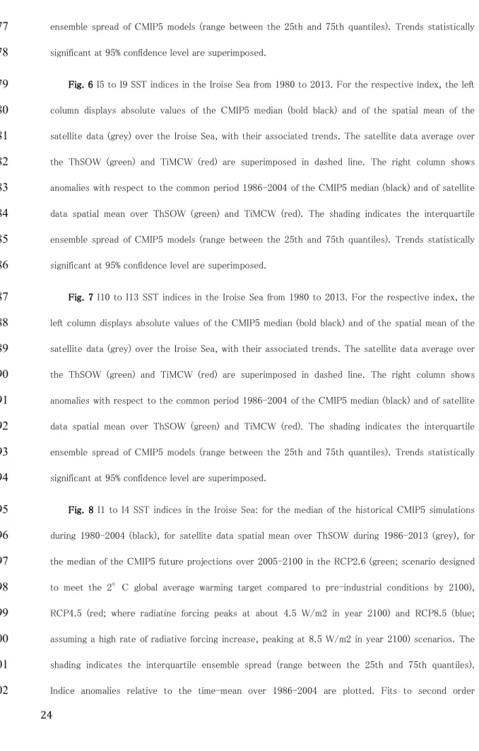
Fig. 5 Fig. 5 Fig. 5

Fig. 5 I1 to I4 SST indices in the Iroise Sea from 1980 to 2013. For the respective index, the left

571

column displays absolute values of the CMIP5 median (bold black) and of the spatial mean of the

572

satellite data (grey) over the Iroise Sea, with their associated trends. The satellite data average over

573

the ThSOW (green) and TiMCW (red) are superimposed in dashed line. The right column shows

574

anomalies with respect to the common period 1986-2004 of the CMIP5 median (black) and of satellite

575

data spatial mean over ThSOW (green) and TiMCW (red). The shading indicates the interquartile