HAL Id: hal-02929461
https://hal.archives-ouvertes.fr/hal-02929461
Submitted on 27 Feb 2021
HAL is a multi-disciplinary open access
archive for the deposit and dissemination of sci-entific research documents, whether they are pub-lished or not. The documents may come from teaching and research institutions in France or abroad, or from public or private research centers.
L’archive ouverte pluridisciplinaire HAL, est destinée au dépôt et à la diffusion de documents scientifiques de niveau recherche, publiés ou non, émanant des établissements d’enseignement et de recherche français ou étrangers, des laboratoires publics ou privés.
Detecting technical anomalies in high-frequency
water-quality data using Artificial Neural Networks
Javier Rodriguez Perez, Catherine Leigh, Benoit Liquet, Claire Kermorvant,
Erin Peterson, Damien Sous, Kerrie Mengersen
To cite this version:
Javier Rodriguez Perez, Catherine Leigh, Benoit Liquet, Claire Kermorvant, Erin Peterson, et al.. Detecting technical anomalies in high-frequency water-quality data using Artificial Neural Networks. Environmental Science and Technology, American Chemical Society, 2020, 54 (21), pp.13719-13730. �10.1021/acs.est.0c04069�. �hal-02929461�
Detecting technical anomalies in
high-frequency water-quality data using
Artificial Neural Networks
Javier Rodriguez-Perez,
†Catherine Leigh,
¶,§,kBenoit Liquet,
†,⊥Claire
Kermorvant,
†,§Erin Peterson,
§,k,#Damien Sous,
†,@and Kerrie Mengersen
∗,†,§,#†Université de Pau et des Pays de l’Adour, E2S UPPA, CNRS, Pau, France ‡Institute for Multidisciplinary Research in Applied Biology, Departamento Ciencias del
Medio Natural, UPNA Pamplona, Spain
¶Biosciences and Food Technology Discipline, School of Science, RMIT University, Bundoora, Australia
§Australian Research Council Centre of Excellence for Mathematical and Statistical Frontiers (ACEMS), Australia
kInstitute for Future Environments, Queensland University of Technology, Brisbane, Australia
⊥Department of Mathematics and Statistics, Macquarie University, Sydney, Australia #School of Mathematical Sciences, Queensland University of Technology, Brisbane,
Australia
@Université de Toulon, Aix Marseille Université, CNRS, IRD, Mediterranean Institute of
Oceanography (MIO), La Garde, France
E-mail: [email protected]
1
Abstract 2
Anomaly detection (AD) in high-volume environmental data requires one to tackle 3
a series of challenges associated with the typical low frequency of anomalous events, 4
the broad-range of possible anomaly types and local non-stationary environmental con-5
ditions, suggesting the need for flexible statistical methods that are able to cope with 6
unbalanced high-volume data problems. Here, we aimed to detect anomalies caused by 7
technical errors in water-quality (turbidity and conductivity) data collected by auto-8
mated in-situ sensors deployed in contrasting riverine and estuarine environments. We 9
first applied a range of Artificial Neural Networks (ANN) that differed in both learning 10
method and hyper-parameter values, then calibrated models using a Bayesian multi-11
objective optimisation procedure, and selected and evaluated the "best" model for each 12
water-quality variable, environment and anomaly type. We found that semi-supervised 13
classification was better able to detect sudden spikes, sudden shifts and small sudden 14
spikes whereas supervised classification had higher accuracy for predicting long-term 15
anomalies associated with drifts and periods of otherwise unexplained high-variability. 16
Introduction
17Monitoring the water quality of rivers is becoming increasingly relevant in the Anthropocene
18
as the need for management strategies to safeguard water resources in human dominated
19
landscapes accelerates. With the advent of new technologies, data on water properties can
20
be obtained with high frequency in near-real time, which can facilitate fast and adaptive
21
management strategies.1,2 However, the generation of high-volume, high-velocity data can
22
create problems of quality control due to a combination of (1) technical issues with the
23
water-quality sensors that result in technical anomalies, and (2) operational problems with
24
traditional, often manual and periodic, methods of quality control that are no longer feasible.
25
In order to improve the quality and utility of high-volumes of data, we therefore need to
26
explore efficient methods to complement or replace traditional methods of quality control,
27
including manual anomaly detection and correction and quality coding.3,4 Improving
quality monitoring will also require robust and flexible statistical methods that can handle
29
data streaming, while also providing big data tools for data-driven decision making.5–7
30
The accurate detection of anomalies in high-frequency, high-volume water-quality data
31
is additionally challenged by several factors. For example, the common low frequency of
32
anomalies in water-quality time series constrains the ability to not only detect anomalies
33
but also to evaluate the performance of detection methods.8,9 There is also a broad range of
34
possible anomaly types, ranging from sudden changes in water-quality values to anomalously
35
constant values maintained for long periods.10,11 In addition, the differentiation of technical
36
anomalies, e.g. related to sensor malfunction or database failure, from the real deviation of
37
the natural system from its typical behaviour is not always straightforward.1 This is because
38
natural fluctuations in environmental conditions at a given site can influence the level of
39
detectability of sensor-related anomalies from the normal signal: the greater the fluctuation,
40
the harder the detection of technical errors. All of these issues can constrain the generality
41
and robustness of detection methods under a broad set of environmental conditions.10,12
42
A combination of methods may be required to address the challenges raised above. For
43
instance, sudden spikes and shifts in values and impossible and/or out-of-sensor-range
val-44
ues on single or just a few observation points can be easily differentiated from adjacent,
45
non-anomalous values. Despite the extremely low frequency of such point-based
anoma-46
lies in time-series data, rule-based, regression-based and feature-based methods may provide
47
optimal performance in terms of their detection.1,11Common anomalies in chemical and
bio-48
chemical data from in-situ sensors also comprise multiple observations, such as sensor drift
49
and periods of unusually high or low variability, which may indicate the need for sensor
cal-50
ibration or maintenance.13 The detection of these multiple-points anomalies can be tackled
51
by various methods,7,11 but remains challenging and often still requires user intervention.
52
Several methods can be combined to extend the range of detected anomalies. Recent work
53
by Leigh et al.11 showed that a combination of rule-, feature and regression-based methods
54
facilitated the correct classification of impossible values, sudden isolated spikes and level
shifts, although drift and periods of high variability still tended to be associated with high
56
rates of false positives.
57
Considering the current global effort to produce real-time, high-frequency and
long-58
term monitoring of aquatic ecosystems, and the limitations of existing quality control
ap-59
proaches,1,4,13 there is a pressing need to explore new methods. Artificial Neural Networks
60
(ANNs) are a promising alternative.6,7,14 One basic strength of ANNs in analysing
high-61
frequency time-series data is that they do not require a priori knowledge of the
underly-62
ing physical and environmental processes. ANNs have therefore been used tackle multiple
63
problems of data streaming including predicting temporal patterns in both marine15,16 and
64
freshwater systems.6,17,18 They have potential to detect anomalies and sudden changes that
65
occur over short-time intervals in water-quality data,6,18,19suggesting that they can be
read-66
ily applied to optimise anomaly detection in complex and fluctuating environmental systems.
67
Previous work on AD applied to water-quality variables compared ANNs to other machine
68
learning methods and found that ANNs have comparable performance to other methods in
69
terms of AD.12,18,20,21 However, authors also acknowledge that remains understudied the
op-70
timisation techniques (especially on those machine learning methods whose learning process
71
depends on a large number of hyper-parameters) that aim to improve detection capacity
72
under real-world conditions.7,20
73
The aim of this study is to test the ability of ANNs to detect technical anomalies in
74
water-quality time-series data in contrasting riverine and estuarine environments. We were
75
especially interested in testing the ability of ANNs to detect multiple-point anomalies, for
76
example those that may result from sensor drift, given that methods previously examined
77
were limited in their ability to accurately detect such context-dependent events. The studied
78
variables are turbidity and conductivity collected at high-frequency by autonomous in-situ
79
sensors. The monitored sites in subtropical Australia and temperate France provide
con-80
trasting ranges of environmental conditions, particularly in terms of the studied variables
81
and their magnitudes and dynamics. The comparison and evaluation of detection methods
in regions that vary in environmental conditions and across a common range of variables
83
is essential to determine the methods’ broad suitability for anomaly detection.7 Given that
84
the environmental fluctuations in each river (freshwater and estuarine sites) may influence
85
the ability to detect the different types of anomalies, we calibrated ANNs using models
86
that differed in learning method and hyper-parameter values. To do so, we implemented a
87
Bayesian optimisation method using a multi-objective approach (i.e. based on scores
spe-88
cially suited to unbalanced classification problems), in order to find the combination of ANN
89
hyper-parameters best suited for anomaly detection at each location. The performance of the
90
calibrated ANNs in detecting different types of anomalies was also evaluated and compared
91
to regression-based methods developed for and applied to similar data.11
92
Materials and Methods
93Study sites
94
The studied water-quality data derive from two freshwater rivers in north eastern Australia,
95
the Pioneer River and Sandy Creek, and an estuarine river in south western France, the
96
Ardour River estuary. Both study areas have seasonality in climate and therefore provide
97
non-stationary environmental conditions of water properties throughout the year.
98
The Australian study area is characterised by humid subtropical climate and strong
99
seasonality: the wet season (typically occurring between December and April) has higher
100
rainfall and air temperatures than the dry season which has lower rainfall and is associated
101
with low to zero river flows.22 Pioneer River (PR) is in the Mackay Whitsunday region of
102
northeast Australia, with a length of 120 km and a monitored catchment area of 1,466 km2,
103
with the upper reaches flowing predominantly through National or State Parks and its middle
104
and lower reaches flowing through land dominated by sugarcane farming. Sandy Creek (SC)
105
is a low-lying coastal-plain stream, 72 km long with a monitored catchment area of 326 km2
106
and with a similar land-use and land-cover profile to that of the lower Pioneer River. Both
study sites are in the freshwater reaches of these rivers.
108
In contrast, south-western France is characterised by an oceanic temperate climate, with
109
drier and warmer conditions from April to October. The Adour River (AR) in the Aquitaine
110
region of southwestern France is 330 km in length and has a catchment area of 16,880
111
km2, with reaches flowing throughout a mosaic of agricultural and forested lands. The
112
study site is in the lower estuary between Bayonne city and the river mouth about 3 km
113
downstream. The tidal range varies from 1 to 4.5 m. Under the combined influence of rainfall
114
and snowmelt during late spring, river flow is highly variable, with minima and maxima of
115
about 80 and 3000 m3/s, respectively.23Driven by such strong fluctuations in tidal range and
116
river discharge, the estuary is classified as a highly variable, time-dependent salt-wedge.23
117
Water-quality data
118
Autonomous multi-parameter in-situ sensors have been installed at each site. At PR and SC,
119
YSI EXO2 sondes with YSI Smart Sensors are housed in flow cells in water-quality monitoring
120
stations on the rivers’ banks. At pre-defined time intervals (see bellow), monitoring systems
121
transport water via a pumping system from the river up to the flow cell. Sensors are equipped
122
with wipers to minimise biofouling and all equipment undergo regular maintenance and
123
calibration, with sensors calibrated and equipment checked approximately every six weeks
124
following manufacturer guidelines. At AR, a YSI 6920 sonde is installed 1 m below the
125
water surface on a floating pier, providing direct measurement of water quality in the river.
126
Data are retrieved during maintenance operations (sensor cleaning, memory erasing, battery
127
replacement) approximately every eight weeks.
128
At each site, the in-situ sensors record turbidity (NTU) and electrical conductivity
(con-129
ductivity; µS/cm). The temporal resolution of data differs among rivers according to local
130
variability in environmental conditions; measurements are taken every 60 and 90 minutes in
131
PR and SC, respectively, and every 10 minutes in the AR. At PR and SC, measurements
132
are sometimes also taken at more frequent intervals during high flow events. The data
quences are one year (12 March 2017 to 12 March 2018) and five months (11 March to
134
13 August 2019) for the Australian and French sites, respectively, totalling 6280, 5402 and
135
14,185 observations at PR, SC and AR, respectively.
136
Water-quality parameters were strongly affected by the non-stationary flow regimes of
137
each site (see Fig. 1). Turbidity is a visual property of water clarity with higher values
138
indicating lower clarity. High turbidity often occurs during flood events, when rivers become
139
loaded with sediment eroded from the catchment, and during local re-suspension events that
140
can result from salt-wedge arrival, flow instability, or navigational and dredging activities.
141
In contrast, low values tend to occur during low discharge periods, e.g. during the dry
142
season, when the slow currents promote sediment deposition or, in estuarine environments,
143
when low-turbidity marine waters have entered the system. These overall trends can become
144
much more complex, and sometimes reversed, under the influence of specific local features.
145
Conductivity reflects the concentration of ions in the water. The dominant effect is generally
146
due to salts, such as sodium chloride, with marine waters typically having much higher
147
conductivity than inland waters. Other dissolved ionic compounds such as nutrients also
148
contribute to conductivity.
149
In the Australian sites, the water regime is driven by rainfall patterns, generating strong
150
positive or negative phases for either turbidity and conductivity values, coinciding with new
151
and sudden inputs of fresh water or periods of low and zero flow (see upper and mid panels in
152
Fig. 1). By contrast, AR is strongly conditioned by the interplay between river discharge and
153
tide forcing. The basic trend is that during high-discharge events, the turbidity reaches high
154
values corresponding to massive seaward fluxes of suspended sediments, and the conductivity
155
is minimal because the marine waters are flushed out from the estuary (see lower panels in
156
Fig. 1). During moderate discharge events, the tidal influence becomes dominant and drives
157
tidal fluctuations of conductivity and turbidity inside the estuary: at high tide, the estuary
158
is filled by salty (high conductivity) and clearer (low turbidity) marine waters while the
159
reverse behaviour is observed at low tide. This pattern is further affected by strong vertical
gradients, the salty marine waters being heavier than fresh riverine waters, which induces
161
complex time-dependent dynamics at the tidal scale.23
162
We focused on turbidity and conductivity data, two common water quality-variables
163
measured in the majority of monitoring programs worldwide and commonly used as proxies
164
of nutrient and/or sediment pollution in rivers, estuaries and marine environments.24 As a
165
global problem, sediment pollution also causes major economic issues related drinking water
166
and dredging.25 In addition, turbidity and conductivity are typically more stable in rivers
167
through time than other properties such as dissolved oxygen and water temperature, which
168
fluctuate daily as well as seasonally.
169
Definitions and types of anomalies
170
Environmental sensors generating high-frequency data sets are usually subject to technical
171
anomalies that can derive from fouling of sensors, sensor calibration shifts, power supply
172
problems or unforeseen environmental conditions that adversely affect the sensor
equip-173
ment.1,26 In general, such technical anomalies strongly depart from the expected pattern of
174
the non-anomalous observations.10 In addition, strong inter- and intra-seasonal variations
175
in environmental conditions from site to site may create local differences in the occurrence
176
and types of anomalies, which can constrain their transferability to other sites.27 We thus
177
need to develop methods for detecting these technical anomalies, that can overcome these
178
challenges,1,11,27 particularly in the context of data streaming.
179
The present analysis focuses on technical anomaly detection (AD) in water-quality time
180
series collected by in-situ sensors. Types of such anomalies have been described1,11 and
181
previous work has indicated the need to explore new statistical methods to better detect the
182
full suite of these types, notably those occurring over multiple, continuous observations (for
183
example as a result of sensor drift), given that such anomalies commonly occur in
water-184
quality time series yet are not as successfully detected as other types of anomalies (e.g.
185
single-point anomalies, out-of-range values).11
Following the framework provided by,11 a range of technical anomalies in the time-series
187
was first identified by local water-quality experts (i.e. for SC and PR by11 and for AR by
188
DS). For each site and variable (i.e. turbidity and conductivity), the identified anomalies
189
were labelled along with their types based on anomaly classes defined by.11 In the present
190
work, we first focused on anomaly types of Class 1 defined as a single observation generating
191
sudden changes in value from the previous observation. Class 1 anomalies were also
consid-192
ered a high priority in terms of detection, given that (true) sudden changes in turbidity and
193
conductivity may be used as early warning signals of water quality by local environmental
194
agencies and that they can strongly influence water-quality assessments and consequent
man-195
agement decisions. We additionally focused on Class 3 anomalies, which include technical
196
anomalies such as long-term calibration offsets and changes comprised of multiple dependent
197
observations. Class 3 was considered lower priority than Class 1 and may require a posteriori
198
user intervention (i.e. after data collection rather than in real time) to confirm observations
199
as anomalous. Specifically, using the nomenclature introduced by,11we based our analyses of
200
AD on those types of Class 1 anomalies defined as (a) large sudden spikes (type A), sudden
201
shifts (type D), small sudden spikes (type J), and Class 3 anomalies defined as drift (type
202
H), high variability (type E) and untrustworthy data not defined by other types (type L).
203
For more information about definitions of each anomaly type and class see.11
204
The present analysis does not focus on AD of those types associated with impossible,
205
out-of-sensor-range and missing values (Class 2) given that they can be easily detected by
206
automated, hard-coded classification rules.11 For each site, we therefore removed all Class
207
2 anomalies from the data prior to analysis. The filtered data were then log-transformed
208
to remove exponential data variance (see Fig. 1) to produce the time-series used for the
209
presented analysis.
Learning methods and data processing
211
One of the most challenging issues for AD in time-series data is that most data are usually
212
"normal" or non-anomalous, while anomalous values are rare.8,9 One of the most common
213
discriminating approaches to solve such a problem is to compare the similarity between
214
two sequences of time-dependent variables, specifically between the sequence of observed
215
and predicted values.11,28 When the anomalous values are pre-labelled, we can apply
semi-216
supervised classification based on training the learning process with the non-anomalous data,
217
fitting models with prediction errors and predicting anomalous events as those observed
218
values falling outside prediction intervals.11,28 Supervised classification feeds the learning
219
process with both a sequence of labelled values for AD (including both anomalous and
non-220
anomalous values, tagged accordingly). The learning process can then generate a sequence
221
of probabilities which can be binary-classified as anomalous or non-anomalous according to
222
a predefined threshold parameter.
223
For each water-quality variable and site, time-series data were partitioned according to
224
each learning process (i.e. semi-supervised or supervised classification). For semi-supervised
225
classification, we retained the "normal" values (i.e. we discarded the anomalous values) and
226
divided the time-series into four contiguous sequences of equal size: namely, two adjacent
227
sequences of values for training and two other adjacent sequences for validation (for details,
228
see Figure S1 in SI). Each pair of contiguous sequences for training or validation comprised
229
one sequence for prediction (predictor variable) followed by an adjacent sequence for the
out-230
come (outcome variable), respectively. For supervised classification, the sequence of values
231
(including both anomalous and "normal" values) for prediction and the sequence of labelled
232
values for AD were each divided into two adjacent sequences of equal length, for training
233
and validation (for details, see Figure S1 in SI). Thus, predictor and outcome variables were
234
composed of one sequence for training followed by an adjacent sequence for validation,
re-235
spectively. Given the proportionally low number of anomalies in our data set, we did not
236
Water quality in each of the studied sites undergoes intra- and interannual variation
238
associated with local, seasonal and annual cycles and stochastic environmental events. We
239
therefore incorporated within our analysis a "sliding window" or moving sequence of values
240
of a defined length along the time series. For each site, the sliding window was defined
241
according to the temporal resolution of data, and was 60, 90 and 10 minutes for PR, SC and
242
AR, respectively (see above). For both predictor and outcome variables, we constructed n×p
243
matrices with various time spans, defining the temporal resolution of time-series data and
244
covering meaningful and regular environmental processes occurring in rivers (e.g. 24 h, 12 h, 6
245
h). For example, the matrices of n×1 reflected the time span of 60, 90 and 10 minutes for PR,
246
SC and AR, respectively, whereas the matrices covering time spans of 24 hours were defined
247
by matrices of n × 24, n × 16 and n × 96 for PR, SC and AR, respectively. The differences
248
in matrix n× columns of each site is a consequence of their differences in the temporal
249
resolutions defined above. For more information about the code and functions to allow data
250
processing and matrix construction, see https://github.com/benoit-liquet/AD_ANN.
251
Metrics for model performance and evaluation
252
To evaluate and compare the classification performance of AD, we calculated the four
cate-253
gories of the confusion matrix (i.e. true and false positives and true and false negatives; T P ,
254
F P, T N, F N, respectively) based on the discrimination threshold value t (typically 0.5; see
255
below for detail on the threshold values we used). From these, we calculated accuracy (Acc),
256
sensitivity (sn) and specificity (sp), and positive and negative predictive values (P P V and
257
N P V, respectively), which allowed us to compare results directly with those of Leigh et al.11
258
Acc = T P + T N T P + F P + T N + F N
sn = T P T P + F N sp = T N T N + F P P P V = T P T P + F P N P V = T N T N + F N
Acc, sn, sp, NP V and P P V range between 0 and 1. sn assesses the probability of
259
determining T P correctly, whereas sp of determining T N correctly. Acc assesses the ability
260
to differentiate T P and T N correctly. Finally, P P V and NP V define the proportion of
261
anomalous versus "normal" observations, specifically the negative and positive predictive
262
values, respectively. When dealing with unbalanced classification problems (i.e. when there
263
are far fewer anomalous than non-anomalous observations), many evaluation metrics are
264
biased towards the majority class, maximising TN classification while minimising TP
classi-265
fication.29,30 We therefore also calculated evaluation metrics specially formulated to provide
266
and optimal classification for both positive and negative values in unbalanced data sets.30
267
The first was balanced accuracy (b.Acc), which is defined as the arithmetic mean between
268
the sn and sp values:
b.Acc = T P/(T P + F N ) + T N/(T N + F P ) 2
The second and third were the F1 and the Matthews Correlation Coefficient (MCC),
270 defined as: 271 f1 = 2 × T P/(T P + F P ) × T N/(T N + F P ) T P/(T P + F P ) + T N/(T N + F P ) M CC = T P × T N − F P × F N p(T P + F P ) × (T P + F N) × (F P + T N) × (T N + F N)
Specifically, f1 is the harmonic mean between the sn and P P V , ranging between 1 (i.e.
272
perfect precision and recall) and 0. MCC ranges between -1 (i.e. total disagreement between
273
predictions and observations), 0 (i.e. random prediction) and +1 (i.e. perfect prediction and
274
balanced ratios of the four confusion matrix categories).
275
Artificial Neural Networks and their implementation in time-series
276
AD
277
Artificial Neural Networks (ANN) are machine learning methods, in which neurons (the basic
278
unit of the learning process) are typically aggregated in layers that generate connections
279
between input and output data. The typical structure of an ANN comprises input, hidden
280
and output layers, usually connected sequentially. The input layer contains the observed
281
data as variables (input neurons) and the output layer the predicted values (output or target
282
neurons).31The input and output layers are connected by hidden layers, and the relationships
283
between the neurons are set by non-linear activation functions. For building and checking
the performance of different types of model structure (i.e. the network structure typically
285
associated with the number of layers and neurons), the ANN must be trained, by which the
286
weights associated with connections between neurons are optimised using various methods
287
and training algorithms.
288
A special case of ANNs adapted to time series applications are Recurrent Neural
Net-289
works (RNN), which can be considered a special case of Auto-Regressive Integrated
Mov-290
ing Average (ARIMA) and non-linear autoregressive moving average (NARMA) models.32
291
RNN architecture mimics the cyclical connectivity of neurons, making them well suited for
292
the analysis and prediction of non-stationary time series.33–35 Long Short-Term Memory
293
(LSTM) networks are a re-design of the RNNs capable of learning long-term correlations in
294
a sequence.36 LSTMs are structured in network units known as memory blocks composed
295
of self-connected memory cells and three multiplicative units, namely the "input", "output"
296
and "forget gates" connected to all cells within each memory block.34 Unlike RNNs, LSTM
297
avoids the "vanishing gradients problem", that is when the error signal is used to train,
298
meaning that the network exponentially decreases the further one goes backwards in the
299
network, by means of the gates of the network units.37 As a result, LSTMs allow the model
300
to be trained successfully using backpropagation through time, which is key for accounting
301
for long-term dependent time-series sequences. Although we applied LSTM in subsequent
302
analyses, we use the more generic term ANN from this point onwards.
303
In this study, ANNs were computed and fitted with "Keras", a model-level library which
304
provides high-level building for programming for developing deep-learning models. "Keras"
305
allows the implementation of a wide variety of neural-network building blocks (e.g. layers,
306
activation functions, optimisers) and supports the latest and most effective advances in deep
307
network training (including recurrent neural networks).38 "Keras" is a high-level wrapper of
308
"TensorFlow" and helps to provide a simplified way of building neural networks from
stan-309
dard types of layers while facilitating a reproducible platform for developing deep learning
310
approaches in computational environmental sciences.39 "Keras" is written in "Python" and
the "Keras" package provides an "R" interface to the deep-learning native functions.40
312
In each model run, we compiled a model with a pre-defined set of hyper-parameters (see
313
below), in which the internal model parameters were iteratively updated throughout the
314
training steps (epochs; for definitions of ANNs hyper-parameters, see Text S1 in SI). During
315
each model run, iterations were computed until the error from the model was minimised or
316
reached a pre-defined value. In order to assess the performance of the learning process, we
317
used a pre-defined set of standard metrics of "Keras" commonly used for classification and
318
regression problems. Specifically, for both training and validation data sets, we calculated the
319
loss function for semi-supervised classification and the mean-square error and the accuracy for
320
supervised classification. For each model run, we accounted for over-fitting using learning
321
curves which showed how error changes as the training set size increases.37 To do so, we
322
compared the shape and dynamics of the learning curves of the training and validation data,
323
which can be used to diagnose the bias and variance of the learning process. For instance,
324
the "training learning curve" is calculated from the training data and provided information
325
on the learning process, whereas the "validation learning curve" is calculated from the
hold-326
out data and gives information on the model generality. For details of the dynamics of
327
the learning curves for either semi-supervised and supervised classification with our data
328
sets, see Supporting Information (SI). SI contains the code and R functions to allow the
329
implementation of ANNs using "Keras" in the "R" statistical language.41
330
Optimisation of hyper-parameters and their influence on AD
perfor-331
mance
332
ANNs include a broad suite of hyper-parameters that affect the ability to learn patterns
333
from the data and the performance of model predictions. Before training, we selected ten
334
hyper-parameters that affect (i) the network structure and (ii) the training algorithm; see SI
335
for details on parameter definitions. Furthermore, we defined two additional
hyper-336
parameters related to (iii) the "sliding window" defined by n × p matrices delimited at
regular temporal intervals (see above) and (iv) the "threshold classification" as a measure
338
of the discrimination threshold value to compute the four categories of the confusion matrix
339
(see above). For each hyper-parameter we then defined a range of values (see details in SI)
340
that affect the performance of ANNs. The range of values depended on the type of the
341
hyper-parameter and varied from a continuous searching space (for those hyper-parameters
342
characterised by double precision, such as the learning rate) and discrete values (for those
343
defined by integer values, such as number of layers or units, and functions or algorithms,
344
such as the optimisation algorithm). In the case of the "sliding window" we decided to use
345
discrete values, defining the temporal resolution of the recorded time-series sequence and
346
covering meaningful and regular environmental processes occurring in rivers (e.g. 24 h, 12
347
h, 6 h). For more information about this issue, see SI.
348
Given the large number of possible models to be tested with all the combinations of
349
hyper-parameter values, we tuned the ANN models using a Bayesian optimisation method,
350
which is a common class of optimisation methods, especially in deep-learning networks.42The
351
Bayesian optimisation method works by constructing a posterior distribution of functions
352
(assuming a Gaussian process) associated with the variability of each hyper-parameter, which
353
best describes the "objective function", defined as the "cost" associated with the optimisation
354
problem. With each iteration of the algorithm, the posterior distribution improves and
355
the algorithm becomes more accurate in those regions of the parameter space with higher
356
likelihood to maximise or minimise the objective function.42 The Bayesian statistical model
357
comprises two components: (i) a Bayesian statistical model for modelling the objective
358
function, and (ii) an acquisition function for deciding where to sample next. In our case, we
359
applied the mlrMBO toolbox implemented in the R statistical language. Compared with
360
other black-box benchmark optimisers, the mlrMBO toolbox performs well for expensive
361
optimisation scenarios for single- and multi-objective optimisation tasks, with continuous or
362
mixed parameter spaces.43
363
Our aim for the optimisation procedure was to find combinations of hyper-parameters
that resulted in the best performance for AD classification (see above). The optimisation
365
procedure followed two steps, firstly generating a random search space and secondly focusing
366
on search shrinks, based on the results generated during the random search. First, we started
367
the algorithm by generating a random design (n = 250), which included a varying number of
368
hyperparameters with the aim to generate enough variability to detect the most promising
369
values. In our case we generated iterations by varying randomly the parameter combinations
370
of the 12 hyper-parameters. After computing the model and the optimisation scores of each
371
iteration, we secondly focused on search shrinks of the search space following a Bayesian
372
optimisation method with n = 250 iterations based on maximising performance metrics or
373
objective functions. In our case, we followed a multi-objective Bayesian optimisation method
374
based on maximising, in each k iteration run, the value of b.Acc, f1 and MCC scores,
375
defined above. Such an approach allowed us to maximise the different and complementary
376
properties summarised by each score for unbalanced classification. Following the
multi-377
objective Bayesian method, the optimisation resulted in a total of n = 500 iterations (i.e.
378
n = 250 for random search and n = 250 for Bayesian optimisation) for each combination of
379
water-quality variables, sites and learning procedures.
380
To examine the effects of hyper-parameters predictor variables (hyper-parameters) on
381
the dependent variables (performance metrics), we applied methods for causal inference
382
using random forests.44Specifically, we determined the statistical importance of each
hyper-383
parameter as a predictor on the dependent variables or optimisation scores (e.g. b.Acc, f1 or
384
M CC) by calculating the "Variable Importance" (V I). V I reflects the model performance
385
across the entire range of predictor and response variables, converted into a set of ordinal
386
ranks. V I can be further used to test how the model response changes as the value of
387
any of the predictor variables is changed, meaning that V I is similar to a standard
"one-388
parameter-at-a-time" sensitivity analysis.45 For each hyper-parameter, we computed V I to
389
measure the relative importance (or dependence, or contribution) of such hyper-parameter
390
predictor variables in terms of their effect on optimisation scores. In our case, we computed
the out-of-bag error, which is an error estimation technique used to evaluate the accuracy of
392
a random forest after permuting each predictor variable. We used the R statistical language
393
and the "randomForest" library.46
394
For each water-quality variable and site, we retained the "best" model as that which
395
maximised the optimisation scores. Specifically, for the complete set of candidate models,
396
we averaged the value of b.Acc, f1 or MCC and we retained the "best" model as that
397
maximising the averaged optimisation scores. We compared the shape and dynamics of the
398
learning curves from the "best" models (a) to diagnose whether or not the training and
399
validation data sets were sufficiently representative (i.e. one data set could capture the
400
statistical characteristics relative to other data sets) and (b) to test the behaviour of the
401
learning process (i.e. underfit, overfit, good fit).
402
Results
403Hyper-parameters optimisation for AD
404
The learning rate for AD stabilised early in the optimisation of ANN models, with few
405
improvements on the performance beyond n = 200 model iterations (although see the ANN
406
model for conductivity at SC). For semi-supervised classification, the costs of computing
407
ranged from 0.312 h for turbidity in SC and 3.53 h for turbidity in AR, whereas for supervised
408
classification the cost ranged from 1.11 h for conductivity in PR and 99.5 h turbidity in
409
AR after n = 500 model iterations (see Table S2 in SI). Comparing learning methods,
410
supervised classification had better performance and generated consistently higher values for
411
b.Acc, f1 or MCC, showing a similar and consistent pattern of the accumulative curve along
412
the optimisation process (Fig. 2). Compared to supervised classification, semi-supervised
413
classification required a larger number of model iterations for maximising any of the three
414
performance metrics, notably for turbidity in SC and AR.
415
re-spect to V I of those hyper-parameters affecting optimisation scores. Overall, the "Learning
417
hyper-parameters" had higher V I values than "Model hyper-parameters" for model
perfor-418
mance (see Tables S2 to S4 in SI). In addition, th.class had higher V I in semi-supervised
419
classification, whereas s.win had minor V U for both supervised and semi-supervised
clas-420
sification. Specifically, the hyper-parameters with higher V I for b.Acc, f1 and MCC,
re-421
spectively, were th.class (78.2, 78.4 and 76.5, respectively; V I values averaged across sites,
422
learning methods and water-quality variables), dropout (46.2, 47.8 and 49.0), b.size (43.5,
423
48.4 and 51.8), momen (31.8, 34.3 and 36.2), l.rate (31.3, 33.2 and 35.6). Comparing
learn-424
ing methods, we found that V I of hyper-parameters differed depending on the combination
425
of types of anomalies and water-quality variables. For instance, semi-supervised
classifi-426
cation had higher V I values for th.class, dropout, momen and l.rate, whereas supervised
427
classification for b.size and activ. Comparing sites, th.class had the highest V I values in
428
semi-supervised classification for conductivity in PR, dropout and l.rate in semi-supervised
429
classification for turbidity in SC, b.size for supervised classification for turbidity in PR,
430
momenfor semi-supervised classification for turbidity in AR and activ for supervised
classi-431
fication for turbidity in AR. For details of the V I of those hyper-parameters independently
432
affecting b.Acc, f1 and MCC, see Tables S3 to S5 in SI.
433
After hyper-parameter optimisation, the "best" models also had performed well in terms
434
of b.Acc, f1 and MCC scores, for all water-quality variables and learning methods; Table 1);
435
for details of hyper-parameters and values of the best models, see SI. However semi-supervised
436
classification had less balanced predictions (i.e. lower values for b.Acc, f1 score and MCC)
437
than supervised classification, meaning that anomaly cases (positives) were proportionally
438
less-correctly predicted than "normal" cases (negatives). Specifically, semi-supervised
classi-439
fication had lower rates of TP that we classified as true (sn = 0.652; values averaged across
440
sites and water-quality variables) and lower proportions of positives and negatives that were
441
true (P P V = 0.512), and that generated a moderately balanced detection rate for either
442
TP and TN results (b.Acc = 0.757, f1 = 0.490 and MCC = 0.665). By contrast, supervised
classification provided a higher and balanced detection rate for both TP and TN (b.Acc =
444
0.822, f1 = 0.622 and MCC = 0.762), and thus anomaly cases (positives) were as predicted
445
correctly as "normal" cases (negatives). In contrast, supervised classification had higher
446
detection rates of TP (sn = 0.704) and higher rates of correct classification of TP and TN
447
(P P V = 0.643). For detailed information about the performance of each model, see Table
448
1.
449
For "best" models, we additionally checked that our training and validation data sets were
450
sufficiently representative, based on the learning process of either training or validation data.
451
Overall, we found strong variation for each water-quality variable, site and learning method,
452
suggesting that the presence of certain types of anomalies were not always consistent between
453
training and validation data sets. Both for semi-supervised and supervised classification, we
454
found that the validation data were easier to predict than training data (i.e. the "training
455
learning curve" had poorer performance than the "validation learning curve"), suggesting
456
that the validation data had lower complexity of anomaly types; for details of learning curves,
457
see Fig. S2 to S5 in SI. For supervised classification, we additionally found that the validation
458
data were unable to produce a good fit (i.e. both training and validation learning curves were
459
almost flat), probably as a combination of the low number of anomaly cases (conductivity
460
in PR; see Fig. 1 and Fig. S8 in SI) and the presence of a long-term anomaly event at the
461
end of the data (turbidity in AR; see Fig. 1 and Fig. S9 in SI); the latter pattern did not
462
happen when fitting semi-supervised classification in both data sets, for which the learning
463
process produced a good fit for both training and validation processes. Overall, we did not
464
detect over-fitting of the training data, a result confirmed by the relatively medium-to-low
465
values of dropout (i.e. <0.5) in most of the "best" models (see Tables S2 to S4 in SI for
466
details of the values of hyper-parameters of the "best" models).
AD among types, learning methods and sites
468
Anomaly types of Class 1 were present, but at low abundances, in all water-quality data sets,
469
comprising, on average, 0.137% of cases (Table 2). By contrast, the majority of anomalies
470
were classified as Class 3, which provided 11.6% of cases (Table 2). Anomalies of Class 3
471
were context-dependent with respect to each site and water-quality variable. Specifically,
472
SC had two anomalous periods of high-variability (type E) occurring during the first four
473
months of monitoring (see Fig. 1). PR had two drift sequences (type H) for turbidity and
474
one period of untrustworthy data (type L) and one drift sequence (type H) for conductivity
475
during the first period of monitoring. Finally, AR had a long-drift sequence (type H) at the
476
end of the monitoring period.
477
Comparing the performance of each "best" model with respect to detecting of the
differ-478
ent types of anomalies, we found, on average, that semi-supervised classification had higher
479
capacity for detecting Class 1 anomalies (45.7% vs 23.6% for semi-supervised and supervised
480
classification, respectively; averaged values across sites and water-quality variables), whereas
481
supervised classification had proportionally higher capacity for detecting Class 3 anomalies
482
(72.6% vs 68.8% respectively) (Table 3). However, such differences between learning
meth-483
ods were particularly context-dependent and based on the different combinations of types
484
of anomalies at each site. Semi-supervised classification better detected large-sudden spikes
485
(type A) for turbidity in AR, and small sudden spikes (J) for turbidity in PR and AR.
486
Supervised classification, by contrast, had better performance for detecting drift (type H).
487
Both semi-supervised and supervised classification performed well for detecting high
vari-488
ability (E) and untrustworthy anomalies for turbidity in SC and PR and conductivity in PR.
489
Sudden shifts (type D) for turbidity in SC and drift (H) for conductivity in PR were not
490
detected by any learning method.
Discussion
492In this work we found that Artificial Neural Networks (ANN) provided good classification
493
for AD in high-frequency water-quality data given their ability to deal flexibly with the
494
challenges associated with local environmental variability. We tested the capacity of ANNs
495
for AD under a broad range of variables, anomaly types and real-world conditions. Our
496
data come from separate monitoring programs in different parts of the world and under
497
contrasting environmental systems (i.e. estuarine, freshwater), so our work presents and
498
opportunity to test the robustness and performance of ANNs for AD. We used turbidity
499
and conductivity data, which are commonly measured by water management agencies and
500
monitoring programs, providing an avenue to test other water quality and quantity variables
501
in the future, which may lead to an overall increase in the performance of water-quality
502
monitoring systems. Results of the AD showed that semi-supervised classification was able
503
to cope better with short-term anomalies associated with a single observation or time point
504
than supervised classification, which showed improved performance for detecting anomalies
505
dependent on multiple context-dependent observations.
506
Previous work has shown that regression time-series methods are useful for AD in
sta-507
tionary and non-stationary time-series data sets,,47,48 but the detection of certain anomaly
508
types, such as sensor drift and periods of anomalously high variability, remain challenging.
509
ANNs are a versatile method that can train models using different learning methods, and as
510
shown by our study, can provide the flexibility required to detect a broad suite of anomaly
511
types, including improved performance for detecting extended periods of untrustworthy data.
512
In our case, we applied regression-based and semi-supervised ANNs similarly for AD; that
513
is, models first predict data sequences based on "normal" cases and then classify as
anoma-514
lous cases those departing from a given threshold value. Despite the good performance of
515
ANNs for AD, our findings demonstrate that ANNs could have limitations regardless of
516
the underlying statistical method used and their applicability in near-real time AD. In our
517
perfor-mances, required three orders of magnitude of computing time longer than regression-based
519
ARIMA. Compared to these regression-based time-series methods, the Bayesian optimisation
520
of hyper-parameter values allowed us to optimise classification of anomalies, at the expense
521
of increased computing costs for hyper-parameter optimisation.
522
For the Australian sites, we found that the performance of semi-supervised ANNs
(pro-523
posed here) and regression-based ARIMA (proposed by11) were equivalent in terms of correct
524
classification, notably by providing high false-detection rates (falses) of both anomalies
(pos-525
itives) and "normal" cases (negatives): semi-supervised classification had higher rates of FP
526
and FN which resulted in low values of sn and P P V . We also found that supervised ANNs
527
considerably minimised false detection rates (i.e. low values of FP and FN and maximised
528
snand P P V values), when compared with the regression-based models and semi-supervised
529
ANNs. Semi-supervised ANNs and regression-based ARIMA generated higher rates of false
530
alarms (i.e. both FP and FN), which overestimate anomalous events, than supervised ANNs.
531
We did not detect over-training in the "best" models, but after checking the shape and
532
dynamics of the learning curves we found that the training and validation data sets had
533
inconsistent numbers and presence of anomaly types. For instance, the validation data set
534
in turbidity in AR had a long-term anomaly event which is not present in the training data
535
(see Fig. 1). As a result, there is inconsistency between training and validation data sets
536
in the performance, typically the validation data had higher performance than the training
537
data (see Figs S2 to S5 in SI). The difference in complexity was mainly a consequence of
538
the presence of Class 3 anomalies in the data sets, usually occurring as single long-term
539
anomalous events in each time series. Cross-validation could solve this problem, but it
540
is also true that multiple partitioning of the data sets could have divided the time-series
541
into multiple smaller independent time-series sequences with inconsistent representation of
542
anomaly types among data sets. Multiple partitioning of the time-series sequence could be
543
especially critical during the optimisation process, notably on those hyper-parameters tuning
544
the size of the sub-samples processed during the learning process (i.e. b.size and momen,
and also for s.win). All the above issues were a consequence of the proportionally lower
546
abundance of anomalous events compared to "normal" events in the data sets, a phenomenon
547
that makes the detection of anomalies challenging.
548
We found that semi-supervised ANNs were especially suited to AD of short-term
anoma-549
lous events (i.e. sudden spikes, sudden shifts and small sudden spikes defined as Class 1
550
anomalies, following the terminology of11). Although semi-supervised and supervised ANNs
551
were comparable regarding their ability to detect long-term anomalous events (i.e. drift
552
and periods of high-variability or Class 3 anomalies), the latter had better performance in
553
terms of correct AD (see above). At least for AD of long-term events, our results with
554
ANNs thus outperformed those of regression-based ARIMA,11 which is an important step
555
forward for AD in water-quality data given such anomalies have consistently proved
chal-556
lenging to detect by other automated AD methods. This is because such anomalous, often
557
very context-dependent events can behave similarly to natural, non-stationary water-quality
558
events such that they are only detected manually by a trained eye very familiar with the
559
local conditions. Our novel use of ANNs and Bayesian optimisation for hyper-parameter
560
selection therefore holds much promise for AD in high-frequency water-quality data from a
561
broad range of environments and ecosystems, including rivers, estuaries and marine waters.
562
Although our study is based on the analysis of data from three sites only, it provides
563
a methodological framework for AD in high-frequency water-quality data collected from
564
sites with contrasting non-stationary environmental processes.49,50 We found that the
non-565
stationary environmental conditions of each site played a substantial role in both (i)
deter-566
mining the types of anomalies present and (ii) increasing the uncertainty around the accurate
567
detection of anomalies. The water-quality variables analysed here are affected by long-term
568
environmental processes occurring at each site (i.e. seasonal precipitation patterns in both
569
Australian and French sites), as well as regular and short-term events (e.g. cyclone floods in
570
Australian sites and tidal regimes in the French site). Both short- and long-term
environmen-571
tal processes may interact and this could affected the AD performance. For Australian sites,
the detection of sudden spikes and shifts (i.e. short-term anomalies) and of drifts or periods
573
with high variability (i.e. long-term anomalies) were rarely masked by natural environmental
574
processes (i.e. seasonal rainfall patterns or cyclone floods), and that resulted in the optimal
575
classification of short- and long-term anomalous events by using either semi-supervised and
576
supervised classification, respectively (Table 3). At the French site, by contrast, strong tidal
577
regimes occurred alongside medium-to-high seasonal discharge events, and that conditioned
578
and limited the accuracy of detecting both short- and long-term anomalies (Table 3).
579
In this work, we calibrated ANNs models using Bayesian optimisation of hyper-parameter
580
values, by means of multi-objective optimisation. Although optimisation methodology is
581
well-established for the detection of anomalies in water-quality data,7 multi-objective
op-582
timisation procedures have rarely been applied for AD in time-series analysis for either
583
prediction or detection anomalies using ANNs methods; but see Perelman et al.19 for an
584
application of detecting anomalies using a single-objective optimisation. The application of
585
multi-objective methodology allow us to get a balanced performance of models for
detect-586
ing anomalies in a broad set of environmental conditions. Notwithstanding the potential
587
utility of ANNs for AD demonstrated above, there is substantial room for improvement in
588
the performance under real-world conditions.12 First, we found that the ability for AD is
589
context-dependent, meaning that accuracy is conditioned on the spatio-temporal
environ-590
mental variability of the data set available. Anomalies are rare events, meaning that we
591
need large data sets spanning the entire environmental variability of each locality to ensure
592
their inclusion in a data set.11Second, we performed our detections based on the analysis of
593
independent environmental variables (i.e. turbidity or conductivity), but the application of
594
ANNs with multivariate time-series could enable us to account for the temporal correlation of
595
multiple variables monitored at the same time.19,24,51 Finally, methodological improvements
596
provide additional avenues to increase the performance of ANNs in AD, such as Bayesian
597
RNNs,52,53 which allow quantification of the uncertainty and the use of ensemble
averag-598
ing for ANNs, combining unsupervised and supervised classification54or the combination of
ANNs with other methodologies.6,55
600
The study of AD in high-frequency data has numerous applications in environmental
601
and health monitoring, and fault and fraud detection, where there is a need to provide
602
near-real time solutions and optimal performance for monitoring and to ensure the quality
603
of data streaming. We have demonstrated that ANNs are a flexible method for providing
604
optimal performance for AD, given they are able to cope with both long- and short-term
605
non-stationary processes that condition high-frequency data. However, ANNs and their
606
hyper-parameter optimisation have been understudied in the context of AD in water-quality.
607
Given the promising results from our study, we therefore recommend further investigation
608
and development of such methods to improve the accurate detection of a broad suite using
609
machine learning or deep-learning methods of anomalies detection under a wide range of
610
environmental conditions.7 Environmental data are intrinsically variable though time and
611
space and thus our approach is transferable for AD in complex spatio-temporal applications
612
and ecosystems. Our findings will therefore be of relevance to water scientists and
man-613
agers throughout the world in order to broaden the applicability of ANNs for efficient water
614
monitoring.
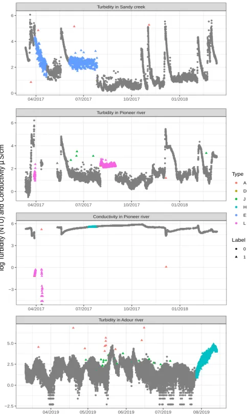
Turbidity in Sandy creek 04/2017 07/2017 10/2017 01/2018 0 2 4 6
Turbidity in Pioneer river
Conductivity in Pioneer river
04/2017 07/2017 10/2017 01/2018 04/2017 07/2017 10/2017 01/2018 −3 0 3 6 0 2 4 6
Turbidity in Adour river
04/2019 05/2019 06/2019 07/2019 08/2019 −2.5 0.0 2.5 5.0 log T
urbidity (NTU) and Conductivity
µ S/cm Type A D J H E L Label 0 1
Figure 1: Observed trends for each water-quality variable and site, including the type of anomaly. Shapes correspond to the different data values (i.e. circles for "normal" values and triangles for anomalous values) and colours to the different anomaly types. Anomaly types were classified by local water-quality experts. For instance, Class 1 anomalies are defined as large sudden spikes (type A), sudden shifts (type D), small sudden spikes (type J), and Class 3 anomalies as drift (type H), high variability (type E) and untrustworthy data not
0.4 0.6 0.8 1.0 0 100 200 300 400 500 k model iterations
Cumm. biased Acc.
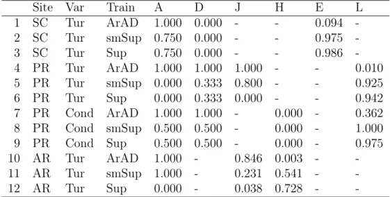
a) 0.00 0.25 0.50 0.75 1.00 0 100 200 300 400 500 k model iterations Cumm. f1−score b) −0.25 0.00 0.25 0.50 0.75 1.00 0 100 200 300 400 500 k model iterations Cumm. MCC c) AR Tur PR Cond PR Tur SC Tur smSup Sup
Figure 2: Cumulative optimisation scores for hyper-parameter optimisation along k model iterations. Each panel showed the procedure of multi-objective optimisation procedure of (a) balanced Accuracy, (b) f1-score and (c) Matthew’s Correlation Coefficient occurring in each k iteration run. The optimisation begins searching with 250 random iterations, and then with 250 iterations of the Bayesian optimization procedure. Colours define each water-quality variable and site, whereas line patterns indicate the learning method. Abbreviations: Sandy creek (SC), Pioneer river (PR) and AR Adour river (AR); Turbidity (Tur) and Conductivity
Acknowledgement
616Funding was provided by the Energy Environment Solutions (E2S-UPPA) consortium and
617
the BIGCEES project from E2S-UPPA ("Big model and Big data in Computational
Ecol-618
ogy and Environmental Sciences"), the Queensland Department of Environment and
Sci-619
ence (DES) and the ARC Centre of Excellence for Mathematical and Statistical Frontiers
620
(ACEMS). A repository of the water-quality data from the in situ sensors used herein and
621
the code used to implement methods of Artificial Neural Networks for anomaly detection are
622
provided in the Supporting Information.
623
Supporting Information Available
624A listing of the contents of each file supplied as Supporting Information are included. The
625
following files are available free of charge.
626
• Figure S1: Scheme of the data processing for time-series AD for each learning method.
627
• Text S1 and Table S1: Brief definition of the parameters and range of
hyper-628
parameter values for fitting and optimising ANN models.
629
• Table S2: Costs of computing time during learning process.
630
• Tables S3 to S5: Variable importance (VI) of values of hyper-parameters to maximise
631
the biased Accuracy, the f1-score and the Matthews Correlation Coefficient.
632
• Figures S2 to S5: Learning curves for semi-supervised and supervised learning processes
633
for the "best" ANN models after Bayesian optimisation.
634
• Figures S6 to S9: Data of observed trend and the probability of anomaly detection for
635
the "best" ANN models after Bayesian optimisation.
636
2Abbreviations: large sudden spikes (A), sudden shifts (D), small sudden spikes (J), and Class 3 anomalies
1: Performance of the best mo del for AD. For eac h site and w ater-qualit y variable, de tails of the hyp er-parameters and values of the best mo del are sho wn in SI .W e calculated performance scores for ARIMA with Anomaly D etection (ArAD), ervised AN Ns (smSup) and sup ervised ANNs classification (Sup). For abbreviations of site s and variables see Figure Site V ar Train TN FN FP TP acc sn sp PPV NPV b_acc f1 MCC SC Tur ArA D 4348 829 134 91 0.822 0.099 0.970 0.404 0.840 0.535 0.16 0.22 SC Tur smSu p 19 97 514 2485 405 0.445 0.441 0.446 0.14 0 0.795 0.443 0.21 0.40 SC Tur Su p 4353 540 117 374 0.878 0.409 0.974 0.762 0.890 0.692 0.53 0.64 PR Tur ArAD 5405 711 144 20 0.864 0.027 0.974 0.122 0.884 0.501 0.04 0.06 PR Tur smSup 3302 43 2180 684 0.642 0.941 0.602 0.239 0.987 0.772 0.38 0.69 PR Tur Sup 5330 49 208 669 0.959 0.932 0.962 0.763 0.991 0.947 0.84 0.97 PR Cond ArAD 5705 448 56 71 0.920 0. 137 0.990 0.559 0.927 0.564 0.22 0.29 PR Cond smSup 2254 1 3410 480 0.445 0.998 0.398 0.123 1.000 0.698 0.22 0.60 PR Cond Sup 6091 0 69 48 0.989 1.000 0.989 0.410 1.000 0. 994 0.58 0.65 AR Tur ArAD 12 744 1573 452 38 0.863 0.024 0.966 0.07 8 0.890 0.495 0.04 0.05 AR Tur smSup 9540 1469 3654 142 0.654 0.088 0.723 0.037 0.86 7 0.406 0.05 0.07 AR Tur Sup 13017 925 179 495 0.924 0.349 0.986 0.734 0.934 0.668 0.47 0.55 1Abbreviations: T rue negativ es (TN), false negativ es (FN), false p ositiv es (FP), true p ositiv es (T P ), accuracy (A cc), sensitivit y (sn), sp ecificit y negativ e prop ortion of v alues (NPV), p ositiv e prop ortion of v alues (P PV ), b a la n ced accuracy (b.Acc ), f1 score (f 1 ) and Matthew’s Correlation efficien t (M C C ).
Table 2: Number of anomalous events according to each type (columns), site and water-quality variable (rows). The anomaly types shown here were classified by local water-water-quality experts, and their classification is detailed in the Material and methods and in Leigh et al.11 For abbreviations of sites, variables and training see Figure 2.
Site Var A D J H E L SC Tur 4 1 0 0 914 0 PR Tur 1 3 5 0 0 718 PR Cond 2 2 0 397 0 80 AR Tur 11 0 26 1574 0 0 2
Table 3: Performance of the "best" model for AD by anomaly type. For each site and water-quality variable, values represent the percentage of data values detected relative to the total number of respective anomalies labelled in the data set (see Table 3 for details). For abbreviations of sites, variables and training see Figure 2 and of anomaly types see Table 2.
Site Var Train A D J H E L 1 SC Tur ArAD 1.000 0.000 - - 0.094 -2 SC Tur smSup 0.750 0.000 - - 0.975 -3 SC Tur Sup 0.750 0.000 - - 0.986 -4 PR Tur ArAD 1.000 1.000 1.000 - - 0.010 5 PR Tur smSup 0.000 0.333 0.800 - - 0.925 6 PR Tur Sup 0.000 0.333 0.000 - - 0.942 7 PR Cond ArAD 1.000 1.000 - 0.000 - 0.362 8 PR Cond smSup 0.500 0.500 - 0.000 - 1.000 9 PR Cond Sup 0.500 0.500 - 0.000 - 0.975 10 AR Tur ArAD 1.000 - 0.846 0.003 - -11 AR Tur smSup 1.000 - 0.231 0.541 - -12 AR Tur Sup 0.000 - 0.038 0.728 -