HAL Id: hal-01537210
https://hal-agroparistech.archives-ouvertes.fr/hal-01537210
Submitted on 14 Jun 2017HAL is a multi-disciplinary open access archive for the deposit and dissemination of
sci-L’archive ouverte pluridisciplinaire HAL, est destinée au dépôt et à la diffusion de documents
Application of neural network modelling for the control
of dewatering and impregnation soaking process
(osmotic dehydration)
Ioan-Cristian Trelea, Anne-Lucie Raoult-Wack, Gilles Trystram
To cite this version:
Ioan-Cristian Trelea, Anne-Lucie Raoult-Wack, Gilles Trystram. Application of neural network modelling for the control of dewatering and impregnation soaking process (osmotic dehydra-tion). Food Science and Technology International, SAGE Publications, 1997, 3 (6), pp.459-465. �10.1177/108201329700300608�. �hal-01537210�
APPLICATION OF NEURAL NETWORK MODELLING FOR THE CONTROL OF DEWATERING AND IMPREGNATION SOAKING PROCESS ("Osmotic
Dehydration")
Docteur Ioan C. TRELEA1, Docteur Anne-Lucie RAOULT-WACK2,
Professor Gilles TRYSTRAM1, 1ENSIA-INRA, 91305 Massy, France
2CIRAD-SAR, BP 5035, 34032 Montpellier, France
Phone (33) 67 61 57 13 – Fax (33) 67 61 12 23 (to whom correspondence should be addressed)
ABSTRACT
The present work aimed at elaborating a predictive modeling of mass transfer (water loss and solute gain) occurring during Dewatering and Soaking Process, with neural network modeling. Two separate feed-forward network with one hidden layer were used (for water loss and solute gain respectively). Model validation was carried out on results previously reported by Raoult-Wack et al. (1991), and dealing with agar gel soaked in sucrose solution, over a wide experimental range (temperature 30 to 70°C, solution concentration 30 to 70 g sucrose/100 g solution, time 0 to 500 min, agar content in the gel 2 to 8 %). Best results were obtained with 3 hidden neurons, which made it possible to predict mass transfer with an accuracy at least as good as the experimental error, over the whole experimental range. Technological interest of such a model is related to rapidity in simulation comparable to a traditional transfer function, limited number of parameters and experimental data involved, and the fact that no preliminary assumption on the underlying mechanisms was needed.
KEY WORDS
INTRODUCTION
The "Dewatering and Impregnation Soaking Process (DIS process)" (Osmotic dehydration) is a technological pre-treatment , which consists in soaking water-rich solid food materials into concentrated aqueous solutions (mainly sugars or salts). This operation leads to simultaneous dewatering, and direct formulation of the product (through impregnation plus leaching).
Industrial applications of Osmotic dehydration has long been restricted to implementation of semi-candied fruit production lines in South East Asia. In this case, osmotic dehydration is operated in batch under normal pressure, beween 30 and 80°C, with sucrose solutions (possibly blended with inverted sugars). Osmotic dehydration is then followed by complementary air-drying.
At present, recent advances obtained in the field of mass transfer control have reinforced the industrial potential of osmotic dehydration. It has been considered more generally as a pretreatment to be introduced in any conventional fruit and vegetable processing chains, in order to improve quality and save energy (Torreggiani, 1993). It can also be be used for meat and fish (Collignan and Raoult-Wack, 1992; Collignan and Raoult-Wack, 1993), and gel materials (Raoult-Wack et al., 1991a; Raoult-Wack, 1991). Recent advances in the field were recently reviewed by Le Maguer (1988), Wack et al. (1992), Torreggiani (1993), and Raoult-Wack (1994).
Most existing models developped in the field of DIS process are diffusional (Hough et
al., 1993), but models based on mass balances (Raoult-Wack et al., 1991b; Azuara et al., 1992)
and more complex models involving the concepts of Irreversible Process Thermodynamics were also studied (Le Maguer and Biswal, 1988).
As a whole, existing models do not permit adequate control of DIS process in industrial applications, because of excessive calculation procedure and number of parameters, but also because they cannot take into account the process complexity. In fact, DIS process implementation generally involves sequential operations with various concentrations and temperatures (Saurel et al., 1995). Moreover, the behaviour of natural tissue subjected to soaking is highly variable, which may be mainly due to the tissue denaturation stage for vegetable (Saurel et al., 1994 a-b), and to fat content for animal tissue (Collignan and Raoult-Wack, 1992). Besides, processing time duration can be as short as one or two minutes, for instance in the case of seaweed (Raoult-Wack and Collignan, 1993).
For the control of DIS process carried out in batch, a dynamic model is necessary for two reasons. The first reason is that development of software sensors (smart sensors) is generally based upon the coupling of a dynamic model with easy to perform measurements. Measurements could be performed on the syrup (which is easier than on food pieces), and the model should be able to predict the evolution of the food pieces properties (water loss, solute gain, stuctural and mechanical modifications,...). The second reason is that design and implementation of control strategies need to predict the further behaviour of product properties, in order to select the best evolution of operating conditions.
There are numerous methods for modelling dynamic processes. In the case of food processes, due to variability and non linear behaviour of natural product, non linear methods are suitable. Neural network are today recognised as good tools for dynamic modelling, and have been extensively studied since the publication of the perceptron identification method (Rumelhart and Zipner, 1985). The interest of such models includes modelling without any assumptions about the nature of underlying mechanisms, and their ability to take into account non linearities and interactions between variables (Bishop, 1994). Recent results establish that it is always possible to identify a neural model based on the perceptron structure, with only one hidden layer, either for steady state or dynamic operations (with recurrent models) (Hornik, 1989 and 1993).
For food processes, the interest in application of neural computing keeps on growing. First applications concerned fermentation (Latrille, 1994) and extrusion processes (Linko et al., 1982), both for control and measurements. Recent papers dealt with filtration (Dornier et al., 1995), and drying (Rocha meir et al., 1994; Huang and Mujumdar, 1993). Some applications were developped in the field of chemical engineering (Bhat et al., 1990) for modelling purposes. For more complex problems, neural computation were used for modelling or sensory description of a food product using its composition (Bardot et al., 1994).
To our knowledge, the use of neural network to control DIS process has never been studied so far . The aim of the present work was to test the interest and efficiency of neural networks to model and predict the behaviour of water rich solid pieces soaked in highly
concentrated solutions. Neural network modelling was elaborated using experimental results obtained by Raoult-Wack et al. (1991a) on agar model gels soaked in sucrose solutions. The objective was to elaborate a predictive model for solute gain and water loss, as a function of experimental conditions : temperature, initial sucrose concentration of the soaking solution, initial agar concentration in the model gel, and time.
MODEL
Network structure
An artificial neural network is an association of elementary cells or "neurons" grouped into distincts layers and interconnected according to a given architecture. The standard network structure for function approximation is the multilayer perceptron (or feed forward network) which we also use in this work.
In figure 1 is presented the network for the solute gain model ; the water loss model is similar. The input layer consists of m=4 identity fan-outs units, one for each input, with no coefficient associated to them. The neurons in the single hidden layer compute a weighted sum of their inputs, and apply a squashing transfer function to the result. The number r=3 of units was selected after some tests. The coefficient associated to the hidden layer are grouped into the matrices A1 (weights) and B1 (biases). The output layer contains p=1 neuron in our case (because there is only one output), which computes the weighted sum of the signals provided by the hidden layer. The associated coefficients are grouped into matrices A2 and B2.
The matrices have the following dimensions : A1∈ℜr×m, B1∈ℜr×1, A2 ∈ℜp×r, B2 ∈ℜp×1,
and the total number of network coefficients is : n = r⋅(m+1) + p⋅(r+1) = 19
Using the matrix notation, the network output can be computed from Eq.(2) :
SG = 100⋅[A2⋅tanh(A1⋅u + B1) + B2] Eq. (2) For further details, the reader is referred to standard textbooks on neural networks (Freeman and Skapura, 1992). Taking into account the normalisation of the inputs and of the outputs, as well as the fact that hyperbolic tangent calculation (if suitably arranged) requires 4 basic floating point operations plus an exponential function calculation, the number Nf of the elementary floating
point operation needed for a neural model simulation is Nf = 2r⋅m+2p⋅r+m+p+4r = 47
and the number of exponential function calculation is Ne = r = 4.
These numbers are very small compared to what is needed for physical models. The simulation of a model based on differential equations for example, typically requires many thousands of floating point operations.
On a standard Pentium based PC computer at 90 MHz, a basic floating point operation takes 0.11 µs, and an exponential calculation 2.2 µs (figures obtained in Matlab, after several tests on large matrices). A neural model simulation thus takes less than 15 µs, which is comparable to traditional linear transfer function and state space models, with the additional advantage of taking into account nonlinear phenomena.
Such networks are universal approximators, provided that a sufficient number of hidden units is used. Other architectures are also considered in literature, with similar properties; for
example Narendra and Parthasaraty (1990) used two hidden layers, while Sanner and Slatine (1992) prefer radial basis transfer functions for the single hidden layer. Let us point out that clear theoretical guidelines for the choice of the structure are lacking, and most authors chose the network structure for a specific application on a trial and error basis.
Identification: learning algorithm
An outstanding feature of neural networks is the ability to learn the solution of the problem (here a multi-input, multi-output mapping) from a set of examples and to provide a smooth and reasonable interpolation for new data (generalization ability). In the field of Food Process Engineering, it is a good alternative to conventional empirical modelling based polynomial and linear regressions. The learning process consists in adjusting the network coefficients (the weight Ai and Bi) in order to minimize an error function (usually a quadratic one) between the network outputs for a given set of inputs and the known correct outputs.
If smooth nonlinearities are used, the gradient of the error function can be easily computed by the classical back propagation procedure (Rumelhart et al., 1986). Early learning algorithms used this gradient directly in a steepest descent optimization, but recent results, as well as our own experience, showed that second order methods are far more effective. In this work, the Levenberg-Marquardt optimization procedure in the Neural Network Toolbox (Demuth and Beale, 1993) was used. Despite the fact that the computations involved in each iteration are more complex than in the steepest descent case, the convergence is faster, typically
by a factor of 100. The learning process is much more computationally intensive than the simulation. If typically takes 5 to 10 minutes on the above mentioned PC computer.
Data bases
Available experimental data are usually divided into the learning data base and the test data base. The learning data base is used for weight adjustment using the learning algorithm. The test data base is used for testing the generalization abilities of the obtained model.
Model quality assessment
The root mean square error (RMSE) between the experimental values and network predictions was used as a criterion of model adequacy. If the data is affected by random white gaussian noise and the model is correct, the RMSE of a large data set equals the noise standard deviation, and it does not make sense to try to further reduce the modelling error. Unfortunately, this value is usually not available beforehand, so the aim was to obtain similar and as low as possible a RMSE, on both learning and test bases.
Network complexity and over-fitting
The network complexity depends on the choice of architecture. One parameter of the network complexity is the total number of adjustable coefficients (network weights and biases). Our own experience, as well as recent studies, showed that the network complexity should be
kept as low as possible in order to ensure the generalization properties. Large networks can always achieve very small RSME on the learning data base, but for the validation, the performance becomes very poor, indicating the fact that the network learned a particular set of examples rather than the underlying trends.
Only the most significant process variables are used as networks inputs. Experiments are designed in order to provide all relevant combinations of input values, because the network behaviour in regions of the input space, where no examples are present, is unpredictable.
If more than one output are considered, it is better to use separate networks for predicting each output rather than one large network, since it reduces training time, improves model accuracy and generalization capabilities. In this work, separate networks were used to predict water loss and sugar gain respectively.
When the choice of input and outputs is realised, the network complexity is depends on the number of hidden units, which is selected after comparison of different structures. This choice is a compromise between the search of the best RMSE on the test base and lowest number of identified parameters.
In this work, experimental data, provided by Raoult-Wack et al. (1991), consisted of mass transfer kinetics (water loss and solute gain) measured on agar gel cubes (initial side dimension : 9.10-3 m) soaked in aqueous sucrose solutions, under constant external conditions,
over 480 minutes. Agar gel was comprised of agar, sucrose and water. The concentration of the occluded solution within the agar network was fixed at 10 g sucrose/ 100g solution, which is a representative level of sugar concentration in most fruits and vegetables. Mass transfer measurements were water loss and solute gain, noted WL and SG respectively, expressed in g/100g initial gel.
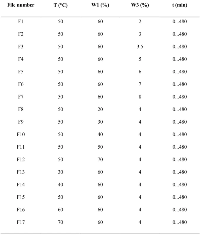
Four process factors were varied: initial agar weight fraction in the gel (noted w3, in %),
processing temperature (noted T, in °C), sucrose weight fraction in the concentrated soaking solution (noted w2, in %), and processing time duration (t, in min.). Table 1 gives experimental
conditions for each of the 17 situations studied. Corresponding files are noted F1 to F17. For each situation, WL and SG measurements were performed at time t= 5, 10, 20, 30, 45, 60, 90, 120, 150, 180, 240, 300, 360, 420, 480 minutes, which resulted in 34 experimental kinetics. Figure 2 presents the distribution of various experimental files in a (T,w2, w3) space.
The selected experimental range is wide, and covers two types of situations, as defined by Raoult-Wack et al. (1991): so-called "dewatering situations", when water loss is higher than sugar gain, and "impregnation situations" in the opposite case.
Experimental files were splitted into learning and test bases, so as to obtain a good representation of the situation diversity ("dewatering" and "impregnation" situations ) in each base, as follows :
- "learning base" : F1, F2, F5, F7, F8, F10, F11, F12, F13, F15, F17 - "test base": F3, F4, F6, F9, F14, F16.
The numerical behaviour of the learning routine is significantly improved if all network inputs and outputs are normalised to similar ranges. This insures that similar importance is given to all inputs and, in the case of a multi-output network, all outputs have similar contributions to the overall error function. Hence, T, w2, WL and SG were divided by 100, w3 by 10 and t by
500. Hence, in Equation (2), u was written as given by Equation (3)
T/100
u = w2/100 Eq. (3)
w3/10 t/500
RESULTS AND DISCUSION
Our model involved 19 weights for 11 kinetics (as calculated by Eq.1), and hence 38 weights for 22 kinetics since there were 2 separate networks.
Figure 3 gives the test RSME respectively, against iteration number in the case of SG, for 1 to 6 neurons in the hidden layer. Results showed that the learning error typically decreased when the number or neurons in the hidden layer increased, but above 6 neurons in the hidden layer, an additional increase in structure complexity does not decrease the learning RSME any more. Figure 3 showed a slight increase in test error, accounting for over-fitting, for more than 30 iterations and 3 neurons in the hidden layer. Let us point out that the increase in test error may be enhanced in other cases. As for water loss, similar behaviour as that previously described for sugar gain was obtained, hence results are not presented here.
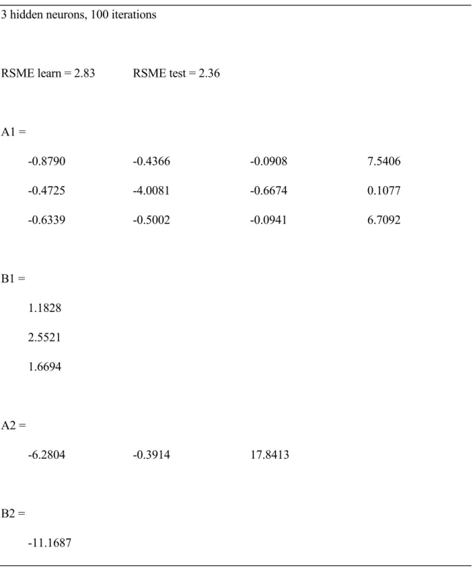
Tables 2 and 3 give the final choice for the number of neurons in the hidden layer (NHL) and iterations, as well as weight values and learning and test RSME, for WL and SG respectively. As a whole, the learning and test RSME were similar, which accounts for a good generalization capability of the neural network. The learning and test RSME are close (even inferior) to experimental error of the original data base and also to that encountered in most studies dealing with the behaviour of real raw materials subjected to DIS process (Saurel et al., 1994 a,b).
Figures 4 and 5 give simulated against experimental data for test and learning bases, for WL and SG respectively. Results showed that in all cases, the prediction is correct, whatever the level of water loss and sugar gain.
Figure 6 gives simulated and experimental WL and SG kinetics obtained in situation F4 (test base ). According to Raoult-Wack et al. (1991a), general time-course evolution could be
divided into 2 phases, which is the typical behaviour in DIS process, whatever the product nature or experimental conditions. In the first phase (0 to 180 min.), WL and SG were very rapid. Then, fluxes progressively decreased, and WL stagnated whereas SG kept on increasing slightly (Phase 2). Simulated results showed that the neural network model provided accurate simulation of WL and SG evolution in both phases.
Figure 7 gives simultaneous simulated and experimental kinetics obtained in situation F9 (test base). As opposed to situation F4, which is a dewatering situation, F9 corresponds to an impregnation situation (SG higher than WL). Results showed that the model satisfiingly described kinetics in each case.
CONCLUSION
This study shows that neural network modelling makes it possible to obtain accurate simulation of water loss and sugar gain kinetics during DIS process, over a wide experimental range, either for dewatering or impregnation situations, with a limited number of parameters and experimental data.
The technological interest of this kind of modeling has to be related to the fact that it is elaborated without any preliminary assumptions on the underlying mechanisms, and also to its implementation facilities, and rapidity in simulation (of order of 15 µs on a standard PC computer).
This neural network modelling was validated on results obtained with model foods. Further modelling should be carried out on real raw materials, and for variable operating conditions. Other architectures ( particularly recurrent ones) should also be studied.
As a whole, in the field of DIS process, the neural model should provide a promising tool for process control in the field of DIS processes. It could also be used for data filtering, which could be of greatest interest in elaborating phenomenological modelling of the process, or typology of the behaviour of materials subjected to soaking from available experimental data, which are claimed to be main shortcomings of research in this field to date.
REFERENCES
Azuara E, Beristain CI, Garcia HS (1992) J. Fd. Sci. Technol. 29 (4), 239-242.
Bardot I, Martin N, Trystram G, Hossenlopp J, Rogeaux M, Bochereau L (1994) A new approach for the formulation of a new beverage. Leben Wiss. und Technol. 27, 503-512. Bhat NV, Minderman PA, MacAvoy T, Wang NS (1990) Modelling Chemecal process systems via neural computation, IEEE Control syst. Magn., April, 24-30.
Bishop CM (1994) Neural networks and their applications. rev. Sci. Instrum. 65 (6) : 1803-1832.
Collignan A, Raoult-Wack AL (1992) Dewatering through immersion in sugar/salt concentrated solutions at low temperature; an interesting alternative for animal foodstuff stabilisation. In: Drying 92, Elsevier. (A.S. Mujumdar ed.), pp. 1887-1897. London
Collignan A, Raoult-Wack AL (1993) Dewatering and salting of cod by immersion in concentrated sugar-salt solutions, Lebensm. -Wiss.u.- Technol. 27: 259-264.
Dornier M, Rocha Meir T, Bardot I, Decloux M, Trystram G (1993) Applications of neural computation for dynamic modelling of food processes; drying and microfiltration.
Artificial intelligence for Agriculture and food. (EC2 ed.), pp. 223-240. Paris.
Demuth H., Beale M.(1993) Neural network toolbox for Matlab- user’s guide, Natrick, MA, The MathWorks Inc.
Hornik (1993) Some new results on Neural Network Approximation. Neural Network, vol 6, 1069-1072.
Hornik K, Stinchcombe M, White H (1989) Multilayer feedforward networks are universal approximators. Neural networks 2: 359-366.
Huang B, Mudjumdar A (1993) Use of neural networks to predict industrial dryers performances. Drying Technol. 11, 525-541.
Freeman J.A., Skapura D.M. (1992). Neural Networks, New york, Addison Wesley.
Latrille E, Corrieu G, Thibault J (1993) pH prediction and final fermentation time determination in lactic acid batch fermentations, In : Escape 2, Coputer chem Eng. 17, S423-428.
Le Maguer M (1988) Osmotic dehydration : review and future directions, In : Proc. of
Symposium on Progress in Food Preservation processes, 1 : 283-309. Brussels.
Linko P, Zhu YH (1992) Neural networks for real time variable estimation and prediction in the control of glucoamylase fermentation, Proc. Biochem. 27, 275-283.
Narendra KS, Parthasaraty K (1990) Identification and control of dynamical systems using neural networks. IEEE trans on neural networks, vol 1, 1, March.
Raoult-Wack AL (1994) Recent advances in the osmotic dehydration of foods. Trends in food science and technology 5 (8): 255-260.
Raoult-Wack AL, Collignan A (1993) Dewatering through immersion in concentrated solutions : an interesting alternative for seafood stabilisation. In : Developments in food
Engineering. (Ed. by T. Yano, R. matsuno and K. Nakamura), Part 1 : pp. 397-400.
Raoult-Wack AL, Guilbert S, Le Maguer M, Rios G (1991-a) Simultaneous water and solute transport in shrinking media. Part 1 : application to dewatering and impregnation soaking analysis (osmotic dehydration). Drying Technol. 9 (3), 589-612.
Raoult-Wack AL, Guilbert S, Lenart A (1992) Recent advances in drying through immersion in concentrated solutions. In : 'Drying of Solids' (Ed. A.S. Mujumdar), pp. 21-51.
Raoult-Wack AL, Petitdemange F, Giroux F, Rios G, Guilbert S, Lebert A (1991-b) Simultaneous water and solute transport in shrinking media. Part 2 : a compartmental model for the control of dewatering and impregnation soaking processes. Drying
Technology 9 (3), 613-630.
Rocha Meir T (1993) Influence des prétraitements et des conditions de séchage sur la couleur et de l'arôme de la menthe et du basilic, Thesis, ENSIA, Massy.
Rosenblatt F (1958) The perceptron: a probabilistic model for information storage and organisation in the brain. Psychol. rev. 65, 386-408.
Rumelhart D, Zipner D (1985) Feature discovering by competitive learning, Cognitive Sc. 9, 75-112.
Sanner RM, Slatine JJE (1992) Gaussian networks for direct adaptive control. IEEE trans
on neural networks, vol 3, 6, Nov., 837-863.
Saurel R, Raoult-Wack AL, Guilbert S, Rios G (1994-a) Mass transfer during osmotic dehydration of apples. part 1 : fresh plant tissue. International Journal of Food Science
and Technology 29: 531-542.
Saurel R, Raoult-Wack AL, Guilbert S, Rios G (1994-b) Mass transfer during osmotic dehydration of apples. part 2 : frozen plant tissue. International Journal of Food Science
and Technology 29: 543-550.
Saurel R, Raoult-Wack AL, Rios G, Guilbert S (1995) Approches nouvelles de la déshydratation-Imprégnation par immersion. IAA 112: 7-13.
Torreggianni D (1993) Osmotic Dehydration in fruit and vegetable processing. Food
1
1
Output layer Hidden layer Input layer T / 100 w2 /100 w3 / 10 t / 500 SG / 100 B2 A131 A114 A111 B11 B13 A23 A22 A2130 40 50 60 70 20 40 60 802 4 6 8 T [°C] w2 [%] w3 [%] F17 F1 F16 F2 F12 F3 F15F4 F11 F5 F14 F10 F6 F13 F7 F9 F8
0 20 40 60 80 100 100 101 102 Levenberg-Maquardt iterations Root-mean square error Test error 1 2 3 6
0 0.1 0.2 0.3 0.4 0.5 0 0.1 0.2 0.3 0.4 0.5 Experimental Simulated LEARN (+), TEST ( )
0 0.1 0.2 0.3 0.4 0.5 0 0.1 0.2 0.3 0.4 0.5 Experimental Simulated
0 100 200 300 400 500 0 10 20 30 40 50 60 70 Time [ i ] Water loss [%], Solute gain [%] File F4
0 100 200 300 400 500 0 10 20 30 40 50 60 70 Time [min] Water loss [%], Solute gain [%] File F9
Table 1 : experimental conditions studied.
File number T (°C) W1 (%) W3 (%) t (min)
F1 F2 F3 F4 F5 F6 F7 F8 F9 F10 F11 F12 F13 F14 F15 F16 F17 50 50 50 50 50 50 50 50 50 50 50 50 30 40 50 60 70 60 60 60 60 60 60 60 20 30 40 50 70 60 60 60 60 60 2 3 3.5 5 6 7 8 4 4 4 4 4 4 4 4 4 4 0...480 0...480 0...480 0...480 0...480 0...480 0...480 0...480 0...480 0...480 0...480 0...480 0...480 0...480 0...480 0...480 0...480
Table 2 : Characteristics of the best neural network in the cases of water loss. 3 hidden neurons, 100 iterations
RSME learn = 2.83 RSME test = 2.36
A1 = -0.8790 -0.4366 -0.0908 7.5406 -0.4725 -4.0081 -0.6674 0.1077 -0.6339 -0.5002 -0.0941 6.7092 B1 = 1.1828 2.5521 1.6694 A2 = -6.2804 -0.3914 17.8413 B2 = -11.1687
Table 3 : Characteristics of the best neural network in the case of solute gain 3 hidden neurons, 30 interations
RSME learn = 2.74 RSME test = 2.60
A1 = -4.3709 4.6844 0.5906 -0.1983 -0.4234 0.4326 -1.4352 -7.6583 -4.5282 5.2997 2.0249 -0.4885 B1 = 0.0000 -1.0218 -0.9562 A2 = 0.7720 -2.0429 -0.6476 B2 = -1.9532
FIGURE CAPTIONS
Figure 1. Schematic representation of the single hidden layer, feed-forward neural network architecture used for the solute gain model. The network used for the water loss model is similar. Figure 2. Distribution of the experimental files in a (T, w2, w3) space.
Figure 3. Test Root Mean Square Error (RMSE) versus iteration number, in the case of solute gain, for various numbers of hidden neurons.
Figure 4. Simulated versus experimental data for test and learning bases, in the case of water loss Figure 5. Simulated versus experimental data for test and learning bases, in the case of solute gain Figure 6. Simulated and experimental kinetics for the water loss (o) and solute gain (+) in the dewatering situation F4.
Figure 7. Simulated and experimental kinetics for the water loss (o) and solute gain (+) in the impregnation situation F9.