A performance analysis of channel fragmentation in dynamic spectrum access systems

(1)

DOI 10.1007/s11134-012-9317-7

A performance analysis of channel fragmentation in dynamic spectrum access systems

Ed Coffman·Philippe Robert·Florian Simatos· Shuzo Tarumi·Gil Zussman

Received: 12 September 2011 / Revised: 8 November 2011 / Published online: 19 June 2012

Abstract Dynamic Spectrum Access systems offer temporarily available spectrum to opportunistic users capable of spreading transmissions over a number of non- contiguous subchannels. Such methods can be highly beneficial in terms of spectrum utilization, but excessive fragmentation degrades performance and hence off-sets the benefits. To get some insight into acceptable levels of fragmentation, we present experimental and analytical results derived from a mathematical model. According to the model, a system operates at capacity serving requests for bandwidth by assigning a collection of one or more gaps of unused bandwidth to each request as bandwidth becomes available. Our main result is a proof that, even if fragments can be arbitrarily small, the system remains stable in the sense that the average total number of fragments remains bounded. Within the class of dynamic fragmentation models, includ-

This paper is a revision for journal publication of the conference paper [3]. All of the results herein can be found in [3].

E. Coffman·S. Tarumi·G. Zussman

Electrical Engineering, Columbia University, New York, NY, USA E. Coffman

e-mail:egc@ee.columbia.edu S. Tarumi

e-mail:shuzo@ee.columbia.edu G. Zussman

e-mail:gil@ee.columbia.edu

P. Robert

INRIA Paris-Rocquencourt, Paris, France e-mail:Philippe.Robert@inria.fr

F. Simatos (

⁾

CWI, Amsterdam, The Netherlands e-mail:florian.simatos@cwi.nl

(2)

ing models of dynamic storage allocation that have been around for many decades, this result appears to be the first of its kind.

In addition, we provide extensive experimental results that describe behavior, at times unexpected, of fragmentation as parameter values are varied. Different scanning rules for searching gaps of available spectrum, all covered by the above stability result, are also studied. Our model applies to dynamic linked-list storage allocation, and provides a novel analysis in that domain. We prove that, interestingly, a version of the 50 % rule of the classical, non-fragmented allocation model holds for the new model as well. Overall, the paper provides insights into the behavior of practical fragmentation algorithms.

Keywords Dynamic spectrum access·Fragmentation·Ergodicity of Markov chains·Cognitive radio·Lyapunov function

Mathematics Subject Classification 60J20

1 Introduction

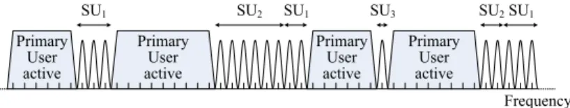
This paper focuses on the analysis of dynamic resource allocation algorithms and is motivated by applications of these algorithms to Dynamic Spectrum Access Net- works (also known as Cognitive Radio Networks). Cognitive Radios can adapt their transmitter parameters to the environment in which they operate and are viewed as key enablers of efficient use of the underutilized wireless spectrum [1,7,8,17]. Un- der the basic model of Cognitive Radio Networks [1], Secondary Users (SUs) are allowed to use white spaces (also known as spectrum holes) that are not used by the Primary Users but must avoid interfering with active Primary Users (for instance, see Fig.1).

An SU’s channel allocation may be broken down into a number of subchannels, each allocated to a distinct hole of unused bandwidth. As shown in Fig.1, this can be realized, for example, by employing a variant of Orthogonal Frequency-Division Multiplexing (OFDM) [10,15,18–20,22]. Although the physical-layer aspects of OFDM-based Dynamic Spectrum Access have been extensively studied recently, al- lowing channel fragmentation introduces several new problems [12,20,23] that sig- nificantly differ from classical Medium Access Control (MAC).¹

Fig. 1 Non-contiguous OFDM with Primary and Secondary Users (SUs), where the Secondary Users use non-contiguous channels that do not overlap with the Primary Users’ channels

1Further details on Dynamic Spectrum Access Networks can be found in [3], which also contains an extensive review of related work.

(3)

In this paper, we study a baseline theoretical model in which the spectrum is shared by SUs only. Those users have to transmit and receive data, and accordingly need some bandwidth for given amounts of time. Hence, bandwidth requests of SUs are characterized by a desired total bandwidth and the duration of a time interval over which it is needed. The data transmission can take place over a non-contiguous channel (i.e., a number of subchannels). Once a transmission terminates, some fragments (subchannels) are vacated, and therefore, gaps (spectrum holes/white spaces) develop randomly in both size and position. When allocating a channel to a new SU request, it is fragmented (in the frequency domain) into available gaps until the full requested bandwidth is provided. This process repeats itself, until the next request fails to fit into the available fragments (more details are provided in the model subsection below).

The main goal of the paper is to investigate the phenomena of fragmentation in- duced by spectrum allocation algorithms. For this purpose, we will ignore the par- ticularities of techniques such as OFDM and make a couple of assumptions (for a complete system description, see Sect.2): (i) the system operates at capacity and there is always a waiting bandwidth request; and (ii) the fragment size is not bounded from below. Making the first assumption allows us to study the effect of fragmentation in the worst case. Clearly, if there are idle periods, when there are no waiting requests, only departures occur and the fragmentation level of the system decreases during these periods. Similarly, the latter assumption allows us to study the system performance when artificial lower bounds on the fragment size are not imposed. This differs from OFDM-based systems in which a subcarrier has a given minimal bandwidth.

In the application of these spectrum allocation algorithms, intriguing new problems in dynamic allocation arise. For example, because of the dynamic use of the spectrum, the bandwidth available to a new user will usually be distributed among a number of gaps in the spectrum. In principle, the random arrival and departure of users might cause the system to evolve in such a way that sequences of many, very small gaps are often allocated to user requests. In such cases, the system performance will deteriorate, since the algorithms maintaining the state of a highly fragmented spectrum become more time-consuming. To put these remarks on a proper footing, we first need to introduce the details of our model.

1.1 The model

A continuous frequency band of given width is made available to users. Each such user makes a request composed of a required total bandwidth and the duration of a residence time for the exchange of data over a channel of this bandwidth. Chan- nels are allocated to requests on a first-come-first-served basis, subject to available bandwidth. A channel must remain fixed while active, and on departure it returns its allocation to the pool of available bandwidth. The channel of an allocated request is allowed to consist of multiple, disjoint bandwidth fragments, each being accommo- dated by a gap of unused spectrum that was available at the time of allocation.

For convenience, the model normalizes the spectrum to the interval[0,1], so the sizes of all bandwidth requests are numbers in[0,1]. Our goal is to characterize the fragmentation of requests when the system is operating at capacity, so we assume that

(4)

there is effectively an infinite queue of waiting users. For the purposes of the example to be given shortly, we denote the sizes of their bandwidth requests byu₁, u₂, . . .. We will also useu_i as the name of theith user. An initial, non-fragmented state is constructed as follows. Starting at 0, consecutive subintervals of sizesu1, u2, . . .are assigned as the channels of waiting users until a request sizeu_i,i >1, is encountered which exceeds available bandwidth, i.e.,

u1+ · · · +ui−1≤1< u1+ · · · +ui

At this point, alli−1 of the channels in this initial state begin their residence times. Subsequent state transitions take place at departure epochs when the residence times of currently allocated channels expire. Suppose all requests up tou_jhave been allocated channels and a requestu_i,i≤j, departs, releasing its allocated channel.

If there is still not enough bandwidth foru_j₊₁, then it must wait for one or more additional departures. Otherwise,u_j₊1, u_j₊2, . . .are allocated their requested band- widths until, once again, a request is encountered that asks for more bandwidth than is available. All channels then begin or continue their residence times as before until the next departure.

The linear-scan (LS) rule sets up a channel by scanning the spectrum in order of increasing frequency, allocating gaps of available bandwidth in partial fulfillment of the request until enough bandwidth has been allocated to satisfy the entire request.

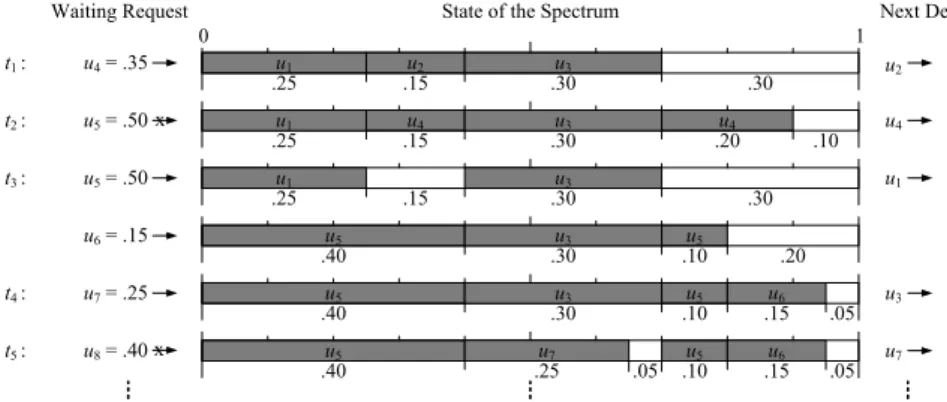
In general, the last gap is only partially used, in which case the last fragment is left- justified in the last gap. An example is shown in Fig.2. Allocations are shown for the first eight user requests, assuming that, at time 0, the spectrum is not in use. The requests with sizesu₁,u₂, andu₃are the first to be allocated channels;u₄must wait for a departure, since the first four request sizes sum to more than 1. The variables t_i give the sequence of departure times of allocated requests. We see that the first occurrence of fragmentation takes place at the departure ofu2 and the subsequent admission ofu4; an initial fragment ofu4is placed in the gap left byu2and a final fragment is placed afteru3. Note also that, even afteru2andu4have departed, there is still not enough bandwidth foru5. After the additional departure ofu1, bothu5and u6, but notu7, can be allocated bandwidth.

Fig. 2 An example of the admission and departure processes and the resulting spectrum fragmentation

(5)

We complete the model description by giving the probability laws governing the residence times and sizes of the waiting requests. Withα∈(0,1]a parameter of the model, the sizesu_j₊₁, u_j₊₂, . . .are drawn independently from the uniform distribution on(0, α]. The residence times of allocated requests are independent of request sizes and form a sequence of i.i.d. exponentially distributed random variables. For simplicity, the mean is normalized to 1.

1.2 Main results

At first glance, since request sizes can be arbitrarily small, the fragments used by bandwidth requests might well become progressively narrower as time passes, in which case the number of fragments could grow without bound. Clearly, such an operational model cannot be supported by a realistic system, so it is of great interest to know whether this can actually happen. The principal theoretical contribution of this paper is a proof that in fact, with high probability, the number of fragments in the system remains acceptably low. A precise statement is deferred to the next section where additional notation and concepts are introduced.

In addition to mathematical results, and in order to gain further insight into the performance of the system, we present the results of extensive experiments. These show that although for a given maximum request sizeα, the number of fragments has a finite expected value, there is a linear relationship between 1/αand the expected number of fragments into which a request is divided. This indicates that when the requests are constrained to be small, they are also fragmented into a relatively large number of fragments. From a practical point of view, this implies that, if we can impose a lower bound on the fragment size by rejecting gaps that are too small, then we have a useful control on the ill effects of excessive fragmentation.

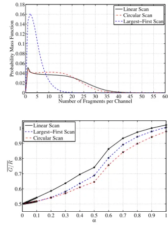
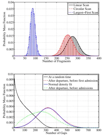
Our experiments show that different bandwidth allocation algorithms exhibit sig- nificantly different performance in terms of the fragmentation occurring in the system. As one example, an algorithm that scans the gaps in decreasing order of their sizes reduces the fragmentation by almost an order of magnitude compared to LS.

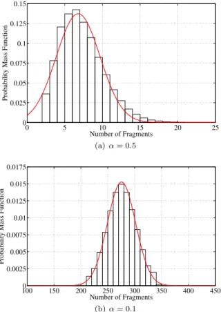
Interestingly, the experiments also show that the number of fragments is distributed according to a normal law with a relatively low mean value. Finally, the experiments for smallα led to the interesting observation that the ratio of the average number of gaps to the average number of requests being served was approximately 1/2. Al- though we were unable to prove this ratio-of-averages result, we were able to prove a corresponding 50 % limit law for the expected value of the ratio of the number of gaps to the number of requests being served.

The spectrum allocation problems described here can be characterized in the context of dynamic storage allocation problems of computers; see Knuth [14]. In that context, the term “spectrum” refers to the storage unit, “bandwidth requirements”

refer to storage requirements, and “channel” refers to a region in storage contain- ing a file. In the original dynamic storage model, fragmentation referred only to the gaps of unoccupied storage interspersed with intervals of occupied storage: files were not fragmented. The reader familiar with that model may have found the 50 % rule observed in our experiments to be reminiscent of Knuth’s 50 % rule, which asserts that the number of gaps is approximately half the number of files when exact

(6)

fits of files into gaps are rare. Our notion of fragmentation applies also to the files themselves, so our discovery that a similar 50 % rule continued to apply was a sur- prising one at first. Note that, in terms of the storage application, our model corre- sponds precisely to linked-list allocation of files—channels allocated to requests are sets of linked, disjoint segments of storage allocated to file fragments. Our results provide a novel analysis for such systems, and have implications for the garbage- collection/defragmentation process in linked-list systems. We note that studies of dynamic storage allocation have been around for some 40 years, and widely recognized as posing very challenging problems to both combinatorial and stochastic modeling and analysis. In particular, results of the type found in this paper, rigorous within stochastic models, seem to be quite new.

The remainder of the paper begins in the next section with the introduction of notation, a formalization of the spectrum state space, and the stochastic processes of interest in later sections. Section3 presents experimental results that bring out the effects of fragmentation, particularly as a function of the maximum request sizeα.

In Sect.4relations between variables describing the configuration of gaps and frag- ments are proved in preparation for (1) a 50 % limit law for the relation between the number of active channels and the number of gaps in the spectrum at departure times, and (2) our main stability result, which shows that the expected value of the total number of fragments and gaps is bounded. These results are proved in Sects.4 and5, respectively. Section 5also proves that, forα large enough, an equilibrium distribution exists. Section6discusses algorithmic issues, such as changes in performance resulting from alternative allocation algorithms, and Sect.7discusses experimental results that exhibit normal approximations for the total number of fragments and gaps. Section8 concludes the paper with a discussion of the results and future research directions.

2 Preliminaries

The state of a fragmentation process must carry the information given by a sequence of gaps alternating with sequences of contiguous fragments. Accordingly, we formalize a state spaceS for our model as follows.

Definition 1 A statex∈Sis given by

x=(L1, . . . , Lr;u)

whereuis the size of the request waiting at the head of the queue,r≥1 is the number of currently active channels, andLiis the list of open subintervals of[0,1]occupied by the fragments of theith channel. Forx to be admissible, the open intervals in

iL_i must be mutually disjoint, and, since the size ofuexceeds the bandwidth available,u >1−

isi has to hold, wheresi is the cumulative size of the fragments inL_i.

Since channel residence times are i.i.d. exponentially distributed random variables, the process(X(t ))onSis a Markov process. The Markov chain embedded at departure timest_nwill be of special interest.

(7)

When treated as a random variable, the size of the request waiting to be allocated bandwidth at timet is denoted byU (t ). Similarly,U_i(t )denotes a random variable giving the size of theith request behind the head of the queue. Except for Sect.5, the dependence on time will usually be omitted. We denote byR(t )the number of requests with an active channel at timet.F (t ) andG(t ) denote, respectively, the numbers of fragments and gaps at timet.

With this notation, we are in position to state our main contribution to mathematical foundations. We prove that the total number of gaps and fragments at departure epochs has bounded exponential moments, as follows: For someη >0 and any initial statex∈S,

sup

n≥1

Ex

e^{η(F (t}ⁿ⁾⁺^G(tⁿ⁾⁾

<+∞

whereExdenotes expectation for the processXstarted atX(0)=x. While our choice of a uniform distribution for request sizes is a useful one, it is not essential to this result; it holds for more general distributions. The result shows that the sumF (t_n)+ G(t_n)is strongly concentrated near the origin. This fact provides strong support for the informal assertion made in Sect.1to the effect that, with high probability, the level of fragmentation stays reasonably low. Our analysis has several basic ingredients:

relations between the number of fragments and gaps in the spectrum (Lemma2); a drift relation of Lyapunov type for the total number of gaps, fragments, and requests (Proposition1); a general inequality for Markov chains (Theorem4); and a stability result of [13].

The last of these results refers to the early work of Kipnis and Robert [13] on a non-fragmented version of our model. Channel allocations can be moved as needed in order to put all available bandwidth together in one block, so fragmentation is avoided entirely. They consider a system with arrivals, but with arrival rates sufficiently high, their analysis of maximum throughput gives us an analysis of(R(tn)), assuming that the same probability laws for request sizes and residence times apply. This follows simply from the fact that the admission criterion for waiting requests is the same in both models. A major result in [13] asserts the existence and uniqueness of an invariant measure for(R(t_n)). Explicit formulas are hard to come by, but those in [13]

for the maximal departure rate in special cases have provided useful checks for our experiments.

In Sect.6, we shall also evaluate two scanning alternatives to LS. The first is cir- cular scan (CS), which is still a linear scan of the gaps, but each scan starts where the previous one left off; after the last gap in[0,1], CS cycles back to the first gap in[0,1]. The second is largest-first-scan (LFS), which is intended to further reduce fragmentation by assigning gaps in order of decreasing size. Although these algorithms make different scans of the gap sequence, they are all alike in their treatment of the last gap occupied: the last fragment is left-justified in the last gap. This is a key assumption, and it is very likely to hold in practice. In our probability model, it follows that, with probability 1, the last gap used in a channel allocation will be changed to a fragment and a smaller residual gap.

(8)

3 Experimental results

The experimental study reported in this section serves two related roles. First, it brings out characteristics of the fragmentation process that need to be borne in mind in implementations, particularly where these characteristics show parameter values that must be avoided, if a system with fragmentation is to operate efficiently. The second role is that of experimental mathematics, in which results indicate where behavior might well be formalized and rigorously proved as a contribution to mathematical foundations. In the latter role, this section leads up to the next two sections, which formalize and prove the stability of the fragmentation process.

The experiments were conducted with a discrete-event simulator written in C that also includes a stochastic arrival process, a capability that we intend to explore in future research. The maximum request sizeα is the single parameter surviving the normalizations of the simpler mathematical model of this paper. The simulations were most demanding, of course, for smallα, when large numbers of departure events were needed to ensure behavior near the stationary regime. For everyαvalue chosen in the interval[0.01,1], 20 million departure events were simulated starting in an empty state, with data collected for the last 10 million events. For every choice ofα in [0.001, 0.01], 100 million departure events were processed and data collection was performed during the last 50 million events. The excellent accuracy of this tool was established in tests against exact results for special classes of queueing systems, and against the maximum throughput results derived in [13]. Examples of the test results can be found in the appendix and in [21].

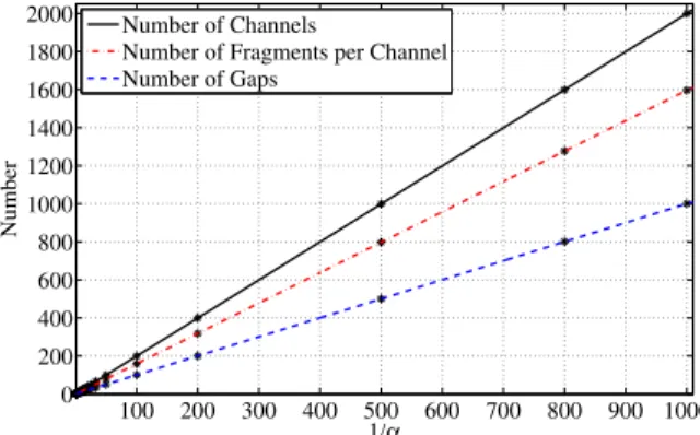
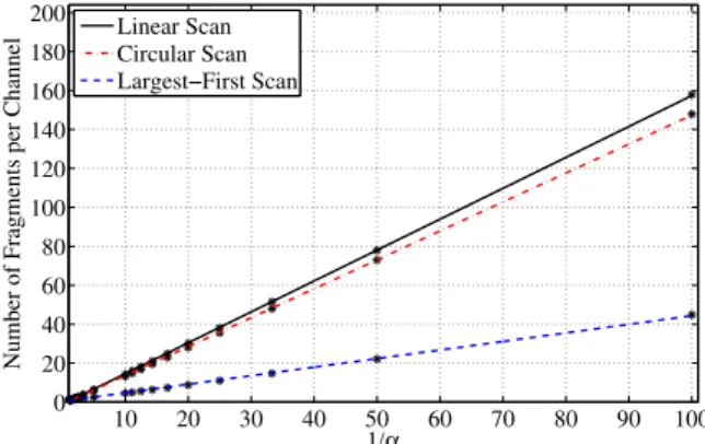
The results for the average number of channels, the average number of gaps, and the average number of fragments per channel are shown in Fig.3. The curves are nearly linear in 1/αfor small values of α; indeed, the errors in the linear fits are within the thickness of the printed lines. In particular, the asymptotic (asα→0) average number of channels in the spectrum is 2/α. When requests are large relative to the spectrum (i.e., forα >1/3), the behavior is not given by functions quite so simple. As such cases are of less practical interest, we omit the relevant data.

The asymptotic linear growth of the average number of channels as a function of channel size is obvious, but the linearity of the other two measures is not so obvious.

A closer look shows that the average number of gaps is almost exactly one half the

Fig. 3 Average numbers of channels, of gaps, and of fragments per channel

(9)

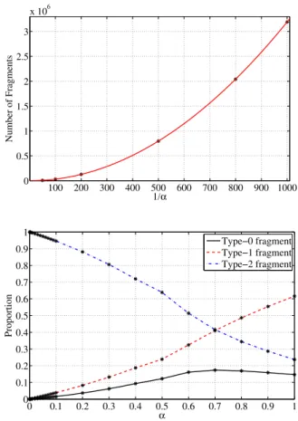
Fig. 4 Average total number of fragments vs.1/α: a quadratic fit

Fig. 5 Percentage of type-i fragments

average number of channels for even relatively small 1/α. This is the unexpected version of Knuth’s 50 % rule that we mentioned in Sect.1. We return to this behavior in the next section, where we prove a 50 % limit law. The linear growth of the average number of fragments per channel may also be unexpected at first glance: the frag- mentation of channels increases as the average channel size decreases. This linear growth implies the quadratic growth of the average total number of fragments plotted in Fig.4(the accuracy of the fit is as before: the error is within the thickness of the printed lines).

The analysis in later sections will focus largely on tracking fragment types defined as follows: a fragment is of typei, if it is adjacent toiother fragments, wherei=0, 1, or 2. It can be seen in Fig.5 that for smallα, more than 90 % of the fragments are type-2 fragments. In addition, clearly, the number of type-0 and type-1 fragments is a function of the number of gaps. These observations and the results illustrated in Figures3and4indicate that, even for relatively small 1/α, the average total number of type-0 and type-1 fragments grows linearly in 1/α, but the average number of type-2 fragments grows quadratically.

Figure6compares the average gap and fragment sizes. As might be expected, for relatively smallα, they are close to each other. The relation holds even for moderately largeα, although forαrather close to 1, the difference amounts to about a factor of 2.

(10)

Fig. 6 Average sizes of fragments and gaps

With this property and the 50 % rule suggested by Fig.3, the linear growth in the number of fragments per channel (shown in Fig.3) is easily explained for moderately smallαin the following way.

As mentioned above, for moderately smallα, the number of channels is approximately 2/α(i.e., the spectrum size divided by the average request size). By the 50 % rule, the number of gaps is roughly 1/α. At any time, the total size of the gaps is at mostα, since there is a request waiting for departures whose requested bandwidth exceeds the total size of the gaps. Therefore, at mostαavailable bandwidth is spread among 1/αgaps, giving an average gap size on the order ofα². The average fragment size is at most (and indeed very close to) the average gap size. The fragments must occupy at least 1−αof the spectrum since, as mentioned above, at most a fraction αof the spectrum is devoted to gaps. Thus, the number of fragments must be on the order of 1/α², and so the average number of fragments per channel must be on the order of (in particular, linear in) 1/α. Asα→0, the asymptotics of these estimates become more precise.

(11)

4 Numbers of fragments and gaps

This section presents analytical results relating the numbers of fragments and gaps under the fragmentation process (X(t )). Recall the definition of fragment types:

Fori=0, 1 or 2, a fragment is said to be of typei if it touches exactly i other fragments.Ni(t )denotes the number of typei fragments at timet, so thatF (t )= N0(t )+N1(t )+N2(t )is the total number of fragments.

Letσ (t )denote the sum of the numbers of fragments and gaps,

σ (t )=F (t )+G(t ). (1)

The number of gaps and the numbers of fragment types are related as follows.

Lemma 1 With probability 1,

G(t )=N₀(t )+1

2N₁(t )+I (t ) (2)

for anyt≥0, whereI (t )=1, if there is a gap starting at the origin, and 0 otherwise.

Proof Each gap, except for boundary gaps starting at 0 or ending at 1, separates two fragments. Two gaps surround a type-0 fragment not touching the origin, only one touches a type-1 fragment not touching the origin, and none touch a type-2 fragment, so the gaps strictly inside(0,1)are double-counted in 2N0(t )+N₁(t ). Gaps at the boundaries are counted only once in this expression, so if there are gaps touching each boundary, 2 must be added to 2N0(t )+N1(t )to produce a double count of all gaps. ThenN₀(t )+N₁(t )/2+1 counts the gaps as called for by the lemma.

With probability 1, a gap always touches the boundary at 1, so the only case left to consider is the absence of a gap touching the origin. In this case, there is a type-0 or type-1 fragment touching the origin, and so a nonexistent gap has been counted in 2N0(t )+N1(t ). This over-count cancels the under-count of the gap touching 1, and so no correction term is needed, i.e.,N0(t )+N1(t )/2 counts all gaps as stated in the

lemma.

Definition 2 Let(t_k)denote the sequence of departure times, letD_i(t_k)denote the number of typeifragments in the channel leaving at timetk, and letA(tk)denote the number of requests admitted to the spectrum at timet_k. Finally, define the drift in the total number of fragments and gaps:

σ (tk)^def=σ (tk)−σ (tk−1) (3) with the conventiont0=Di(t0)=Ai(t0)=0.

The following lemma is the basis of the stability analysis ofσ (t )in Sect.5, and the 50 % rule proved later in this section.

(12)

Lemma 2 With probability 1, the departure att_kcreates the following change in the total number of fragments and gaps:

σ (t_k)=A(t_k)−2D0(t_k)−D1(t_k)+J (t_k), k≥1 (4) witht₀=0, andJ (t_k)=1, if a fragment starting at the origin is in the departing channel, and 0 otherwise.

Proof With probability 1, each new channel allocation covers completely every gap it is allocated, except for the last one, which is only partially covered. Thus, with probability 1, each new channel allocation changes gaps to fragments, except for the last gap which is changed to a fragment plus a gap; this adds one toσ (tk−1)for each admission, which accounts for the total ofA(tk)in (4).

Two fragments of the same channel cannot be contiguous, so it is correct to add up the changes created by departing fragments, with each being treated separately.

Suppose first that there is no fragment(0, b)against the origin. Then for every type-0 fragment in the departing channel, two gaps and a fragment are replaced by a single gap for a net decrease of two, and for every departing type-1 fragment, a gap and a fragment are replaced by a single gap for a net reduction of one. This gives the reduction of 2D0(tk)+D1(tk)appearing in (4). If there is a fragment(0, b), it must be of type 0 or 1; if it is of type 0, then its departure gives a decrease of one; if it is of type 1, its departure has no effect. Each of these contributions is one less than it would be were the fragment not touching the origin. There can only be one such fragment, so the correction shown inJ (t_k)for a fragment(0, b)follows.

We will denote byG⁻(t_k)the total number of gaps just after thekth departure, but before new admissions, if any, are made. Note that if we removeA(t_k)from the right-hand side of (4) and add back the total number of departing fragments att_k, i.e., D₀(t_k)+D₁(t_k)+D₂(t_k), we get the number of gaps available to admissions at the kth departure:

G⁻(t_k)=G(t_k₋1)−D0(t_k)+D2(t_k)+J (t_k) (5) withJ (tk)=1 as in Lemma2.

Knuth’s widely known 50 % rule appears in a very different context than the model here, so it is difficult to anticipate the apparent fact that it also holds for our fragmentation model. However, one can argue a similar result assuming that the fragmentation process has a stationary distribution. The result is given below as an expected value of a ratio, rather than a ratio of expected values.

Theorem 1 Assume that for each α >0, the fragmentation process at departure epochs (X(t_k), k≥0) with request sizes uniformly distributed in (0, α) admits at least one stationary distribution. For eachα >0 pick one stationary distributionπ_α. Then

αlim→0Eπα

G(0) R(0)

=1 2.

(13)

Proof Any stationary distribution π_α must satisfy Eπα[σ (t₁)] =Eπα[σ (t₀)] and Eπα[A(t1)] =1. Thus, using Lemma2one gets

Eπα

2D0(t₁)+D₁(t₁)−J (t₁) =1. (6)

Now for a statexhavingR(0) >0 channels andN_i(0)type-i(i=0,1,2) fragments, we have from Lemma1

Ex

2D0(t₁)+D₁(t₁)−J (t₁) =

2N0(0)+N₁(0)

R(0)−Ex

J (t₁)

=2

G(0)−I (0) R(0)−Ex

J (t1) . The termEx[J (t1)]is equal to the probability that a fragment starting at the origin leaves. This is certainly smaller than the probability that the channel with the fragment closest to the origin leaves, which by symmetry is equal to 1/R(0). Using in additionI (0)=0 or 1 one gets

0≤1 2−Eπ_α

G(0)/R(0)

≤2Eπ_α

1/R(0) .

Now for any stationary distributionπα the random variableR(0)underπα must be distributed according to the stationary distribution of the non-fragmented model of Kipnis and Robert [13], and one easily checks thatEπα(1/R(0))goes to 0 asαgoes

to 0, hence the result.

Note that, because we have a Lyapunov function (see Proposition1), the existence of a stationary distribution would be guaranteed if we could prove that the process(X(t_n))has the Feller property, see for instance Proposition 12.1.3 in Meyn and Tweedie [16].

5 Stability results

This section establishes that the average total number of fragments and gaps remains bounded and that, for certain distributions of request sizes, ergodicity holds. The analysis leads to the following two results. Recall that(t_n)is the sequence of departure times (t0=0) andσ (t )=F (t )+G(t ), defined in (1), is the total number of fragments and gaps.

Theorem 2 There exists someη >0 such that, for any initial statex∈S, sup

n≥1

Ex

e^{ησ (t}ⁿ⁾

<+∞. (7)

Clearly, this implies that for any initial state x ∈S, the sequence (Ex(σ (t_n)), n≥0) is bounded. With an additional assumption on the distribution of the request size, a stronger stability result can be proved.

Theorem 3 Whenα >1/2, the process(X(t ))is positive Harris recurrent; in par- ticular, it has a unique stationary distribution.

(14)

A criterion for finite exponential moments using a Lyapunov function is established next. Then, we provide some estimates of the drift of the number of fragments between departures which will show us how to construct such a Lyapunov function.

The proofs of Theorems2and3will finally be given in Sects.5.4and5.5.

5.1 A criterion for finite exponential moments

Before stating the main result, some results on Markov chains are needed. In the se- quel,≤strefers to stochastic ordering, i.e.,V ≤stZmeans thatE(f (V ))≤E(f (Z)) for any increasing functionf. For reasons that will become clear in Lemma5, the following lemma focuses on admissions at four consecutive departure times. Recall that(U_i, i≥1)are the sizes of the requests waiting to be allocated bandwidth after U, the first one, and that they are assumed to be i.i.d.

Lemma 3 The random variableA(t₁)+ · · · +A(t₄)is stochastically dominated by a random variableZsuch thatE(e^λZ) <+∞for someλ >0.

Proof It is clear thatA(t1)≤Z+1 where

Z=1+inf{n≥1:U1+ · · · +U_n≥1}. Markov’s inequality shows that for anyz≥0,

P(Z≥z+1)=P(U₁+ · · · +U_z≤1)≤e E

e⁻^U¹_z

and soE(e^ηZ)is finite forη >0 small enough. From this observation, it is not difficult to extend the result toA(t₁)+ · · · +A(t₄)instead of justA(t₁).

This lemma shows in particular that ξ^def=sup

i≥1

sup

x∈SEx

A(ti)

<+∞.

is well-defined; this constant will be used repeatedly throughout the rest of the analysis. The proof of the following lemma is standard, and therefore, omitted.

Lemma 4 LetZ≥0 be a positive, real-valued random variable such thatE(e^λZ) <

+∞for someλ >0, and definec=λ⁻²E(e^λZ−1−λZ). Then for any 0≤ε≤λ and any real-valued random variableV such thatV ≤stZ, we haveE(e^εV)≤1+ εE(V )+ε²c.

The following result is closely related to a result of Hajek [11].

Theorem 4 Let(Y_k)be a discrete-time, continuous state-space Markov chain such that for some functionf ≥0, there existK, γ >0 such that for any initial stateywith f (y) > K, the inequalityEy(f (Y₁)−f (Y₀))≤ −γ holds. Assume that there exists a random variableZsuch that for any initial statey,Zdominates stochastically the

(15)

random variablef (Y₁)−f (Y₀)underPy. Assume finally thatE(e^λZ) <+∞for someλ >0. Then there existη >0 and 0≤C <+∞such that for any initial statey,

sup

n≥1Ey

e^{ηf (Y}ⁿ⁾

≤e^{ηf (y)}+C.

Proof For any 0< ε≤λ, Ey

e^{εf (Y}ⁿ⁺¹⁾

=Ey

EY_n

e^{ε(f (Y}¹⁾⁻^{f (Y}⁰⁾⁾

e^{εf (Y}ⁿ⁾1_{_{f (Y}_n₎_≤_K_} +Ey

EYn

e^{ε(f (Y}¹⁾⁻^{f (Y}⁰⁾⁾

e^{εf (Y}ⁿ⁾1_{_{f (Y}_n_)>K_}

. (8)

Since by assumption,f (Y1)−f (Y0)underPyis stochastically dominated byZfor everyy, one gets

EYn

e^{ε(f (Y}¹⁾⁻^{f (Y}⁰⁾⁾

≤E e^εZ

=E e^λZdef

=D and therefore

Ey

EYn

e^{ε(f (Y}¹⁾⁻^{f (Y}⁰⁾⁾

e^{εf (Y}ⁿ⁾1_{_{f (Y}_n₎_≤_K_}

≤De^εK. (9) For the second term, we apply Lemma4to the random variablef (Y1)−f (Y0)under PY_n:

EYn

e^{ε(f (Y}¹⁾⁻^{f (Y}⁰⁾⁾

≤1+εEYn

f (Y₁)−f (Y₀) +cε². Thus, on the event{f (Y_n) > K}, one gets

EYn

e^{ε(f (Y}¹^{)−f (Y}⁰⁾⁾

≤1−γ ε+cε^{2 def}=ρ_ε (10)

and finally Ey

EYn

e^{ε(f (Y}¹⁾⁻^{f (Y}⁰⁾⁾

e^{εf (Y}ⁿ⁾1_{_{f (Y}_n_)>K_}

≤ρ_εEy

e^{εf (Y}ⁿ⁾

. (11)

Gathering the two bounds (9) and (11) in (8) finally gives Ey

e^{εf (Y}ⁿ⁺¹⁾

≤ρεEy

e^{εf (Y}ⁿ⁾

+De^εK

which leads by induction to Ey

e^{εf (Y}ⁿ⁾

≤ρ_εⁿe^{εf (y)}+1−ρ_εⁿ⁺¹ 1−ρ_ε De^εK.

Letη=(ε/(2γ ))∧λ. From the definition ofρ_ε in (10), one can easily check that 0< ρ_η<1. Therefore, choosingε=ηgives the result.

Theorem4will be applied to the Markov chain(X(t4n))with a functionf of the formσ_κ^def=σ+κRfor someκ >0 suitably chosen.(X(t_4n))is not the most natural choice at first glance, but it appears to be needed because of the complexity of the state space.

(16)

By Lemma2,σ (t₁)−σ (t₀)≤A(t₁)+1 and clearlyR(t₁)−R(0)=A(t₁)−1, so that

σκ(t4)−σκ(t0)≤(κ+1)

A(t1)+ · · · +A(t4) +4

and therefore, by Lemma3,σκ(t4)−σκ(t0)is stochastically dominated by some random variableZ with an exponential moment. Therefore, one has to establish a negative drift relation forσ_κ(t₄)−σ_κ(t₀)in order to apply Theorem4 to the fragmentation process(X(t4n)). This is the purpose of the following two subsections.

The most delicate part is to control the termσ (t4)−σ (t0), which is the objective of the following section.

5.2 Evolution of the number of fragments

Letx∈S, the initial state of the system, haveractive channels, and define the total available gap sizeh=1−(s₁+ · · · +s_r). Time 0, referring to the initial statex, will usually be omitted; e.g.,σ (0), F (0), G(0), . . .will be simplified toσ, F, G, . . .. The quantityσ (t_n)is defined in (3) asσ (t_n)−σ (t_n−1).

Lemma 5 Fix 0< ε <1 and 0< η <1/2, and letx∈Sbe an initial state such that σ=G+F ≥2K+1 for some fixedK≥0.

ThenF =N0+N1+N2≥K, and (1) Ifr=1, thenEx(σ (t1))≤ξ−K.

(2) Ifr >1 andN0+N1≥εK, then Ex

σ (t1)

≤ξ+1−εK r .

Assume in the remaining cases thatr >1, defineK=K((1−ε)/r−ε)⁺, and leti^∗∈ {1, . . . , r}index a channelL_i∗inx with the most type-2 fragments.

(3) IfN₀+N₁≤εKandu > h+s_i∗, then Ex

σ (t2)

≤ξ+2− K

r(r−1). (12)

(4) IfN0+N1≤εK,u < h+si^∗andh+si^∗< ηα, then Ex

σ (t₃)

≤ξ+2−(1−η)K

r²(r−1). (13)

(5) IfN0+N1≤εK,u < h+si^∗ andηα < h+si^∗, then there exists aγ (η) >0 such that

Ex

σ (t4)

≤ξ+2−γ (η)K

r⁵ . (14)

It follows that there exists aξ >0 and a functionψ (r) >0 such that for anyx with σ≥2K+1,

Ex

σ (t4)−σ

≤ξ−Kψ (r). (15)

(17)

Proof As is readily verified,G≤F+1, so 2K+1≤σ=F+G≤2F+1, and hence F≥Kas claimed. In what follows, we use repeatedly the two following simple facts:

Ex

D0(t1)+D1(t1)

=(N0+N1)/r, (16) and by Lemma1,

G≥K ⇒ N0+N1≥K−1. (17)

– First case:r=1. In this case, right after the only channel initially present leaves, there is no channel allocated bandwidth, and therefore,σ (t₁)=A(t₁). Note thatr=1 is only possible whenα >1/2, and in this case the possibility for a channel to be alone is crucial in the proof of the Harris recurrence stated in Theorem3.

– Second case:r >1, N0+N1≥εK. Under these assumptions, the inequality follows from (4):

Ex

σ (t₁)

≤ξ+1−Ex

D₀(t₁)+D₁(t₁)

=ξ+1−N0+N1

r ≤ξ+1−εK r . In the 3 remaining cases, let N_j^∗ denote the number of type-j fragments in any channel i^∗ which has the most type-2 fragments. If N₀+N₁≤ εK, then sinceF ≥K, necessarilyN₂≥(1−ε)K andN₂^∗≥(1−ε)K/r. Define the event D^∗= {channelL_i∗leaves att1}and recall thatG⁻denotes the number of gaps right afterL_i∗leaves but before new admissions, if any, are made. It follows from (5) that G⁻≥Kin the eventD^∗, since

G⁻=G−N₀^∗+N₁^∗+J (t1)≥

−εK+(1−ε)K/r₊

=K.

The remaining analysis tacitly assumes thatr >1, thatN0+N1≤εK, and that the channelLi^∗leaves att1.

– Third case:u > h+s_i∗. Under this condition,A(t₁)=0, since whenL_i∗leaves it does not provide enough additional bandwidth forU. In particular,R(t₁)=r−1 andG(t1)=G⁻≥K, and so

Ex

σ (t2)

≤ξ+1−Ex

D0(t2)+D1(t2);D^∗ .

The strong Markov property makes it possible to lower-bound this last term.

Ex

D0(t2)+D1(t2);D^∗

=Ex

EX(t1)

D0(t1)+D1(t1)

;D^∗

=Ex

(N1+N2)(t1) R(t₁) ;D^∗

≥K−1 r−1 Px

D^∗

= K−1 r(r−1) and therefore,Ex(σ (t2))≤ξ+2−K/(r(r−1)).

– Fourth case:u < h+s_i∗< ηα. In this caseU is admitted att₁. Thus it makes sense to define the event

E₄=D^∗∩ {Uleaves att₂andU₁> ηα}.

(18)

Then as before Ex

σ (t3)

≤ξ+1−Ex

D0(t3)+D1(t3);E4

.

In the eventE4,Uis admitted att1and leaves att2, whileU1stays blocked att1and t₂, so thatG(t₂)=G⁻≥KandR(t₂)=r−1. Hence as in the second case,

Ex

D₀(t₃)+D₁(t₃);E₄

≥K−1

r−1 Px(E₄)≥(1−η)K r²(r−1) −1 sincePx(E₄)=(1−η)/r². Thus (13) holds.

– Fifth case:u < h+si^∗andηα < h+si^∗. Again,Uis admitted att1. LettingUi

denote the sizes of the requests behindU, define the event B= {U_i< ηα, i=1, . . . , τ andU_τ₊₁>2ηα}

with τ =inf{n ≥ 0 : U1 + · · · +Un > h+si^∗ − ηα} and E₅ =D^∗ ∩ B ∩ {Uleaves att2}. It is readily verified that 1≤τ <+∞ almost surely. Moreover, one has inE₅

0< h^∗^def=h+si^∗−(U1+ · · · +Uτ) < ηα < Uτ+1.

This means that att2, exactlyτ new requestsU1, . . . , U_τ have been admitted, and U_τ₊₁is blocked. Moreover, for anyi∈ {1, . . . , τ}, one hash^∗+U_i <2ηα < Uτ+1, so that if one of theτ channels allocated to the(Ui)leaves,Uτ+1remains blocked.

WhenLi^∗left, there wereG⁻≥Kgaps; in the remainder of the analysis, we call an initial gap a gap present right afterL_i∗left. AfterL_i∗ left,U andA(t1)−1 new requests were admitted, and thenU left andA(t₂)new requests were admitted att₂. Thus, att2, each initial gap is in either of two states: either it is completely filled, or it is still a gap, i.e., it has not been filled completely. Letkbe the number of initial gaps completely filled att2, and letk=G⁻−k: thenk+k=G⁻≥K. In each initial gap completely covered att₂, there is at least one type-2 fragment of one of theτnew channels. Therefore,N1,2+N2,2+ · · · +Nτ,2≥kwithNi,2the number of type-2 fragments of the channel corresponding toU. In particular there is a channel L_j∗,j^∗∈ {1, . . . , τ}with at least the averagek/τ of type-2 fragments:N_j∗,2≥k/τ. Define finally the eventE₅=E₅ ∩ {L_j∗leaves att₃}. Sinceh^∗+U_j∗< U_τ₊₁, then Uτ+1remains blocked att3whenE5occurs, and therefore (note that whenj^∗leaves, some gaps may merge, but not two initial gaps),

G(t₃)≥N_j∗,2+k≥k/τ+k≥ k+k

/τ ≥K/τ.

Now we proceed as before to obtain Ex

σ (t4)

≤ξ+1−Ex

D0(t4)+D1(t4);E5

and, using the Markov property at timet₃,

(19)

Ex

D₀(t₄)+D₁(t₄);E₅

=Ex

EX(t3)

D₀(t₁)+D₁(t₁)

;E₅

=Ex

(N₀+N₂)(t₃) R(t₃) ;E5

≥Ex

(K/τ−1)⁺ r+τ−2 ;E5

sinceR(t₃)=r+τ −2 inE₅. The same kind of reasoning as before then leads to Ex

(K/τ−1)⁺ r+τ−2 ;E₅

≥K

r⁵f (η, h+s_i∗−αη)−1 with the functionf (η,·)defined fory >0 by

f (η, y)=E

1+τ (y)₋5

;B(η, y)

withτ (y)=inf{n≥1:U1+ · · · +U_n≥y}and B(η, y)=

U_i< ηα, i=1, . . . , τ (y)andU_{τ (y)}₊1>2ηα .

It is not difficult to show that γ (η)=inf0<y<1f (η, y) >0, which then gives the result.

It remains to prove (15). One only needs to assemble the various bounds, taking into account thatEx(σ (t_i))≤ξ+1 for anyx∈Sandi≥0, to arrive at 4 separate bounds onEx(σ (t₄)−σ ). For example, using the former bound for the first two terms and the last term ofEx(σ (t4)−σ )=

1≤i≤4Exσ (ti)and then the bound in (13) for the third term, we find that one of the four bounds, which applies whenxsatisfies the inequalities of the fourth case, is

Ex

σ (t₄)−σ

≤4ξ+5−(1−η)K r⁵

Computing the minimum over these bounds withη=1/4 andε=1/r², one ob- tains (15) after settingξ=4ξ+5 and

ψ (r)=ϕ(r) r⁶ ×

(1−η)∧γ

withϕ(r)=1−2r⁻². This concludes the proof.

The bound (15) gives a negative drift for σ when the termKψ (R(0)) is large enough. Butψ (r)vanishes whenrgoes to infinity, and so this bound cannot yield a drift uniformly negative, the problem occurring whenR(0)is large. For this reason σ is not a Lyapunov function but the simple modificationσκ=σ+κR introduced earlier is. The purpose of the additional termκRis precisely to give a negative drift whenR(0)is large.