HAL Id: hal-03173080
https://hal.archives-ouvertes.fr/hal-03173080
Submitted on 18 Mar 2021
HAL is a multi-disciplinary open access
archive for the deposit and dissemination of
sci-entific research documents, whether they are
pub-lished or not. The documents may come from
teaching and research institutions in France or
abroad, or from public or private research centers.
L’archive ouverte pluridisciplinaire HAL, est
destinée au dépôt et à la diffusion de documents
scientifiques de niveau recherche, publiés ou non,
émanant des établissements d’enseignement et de
recherche français ou étrangers, des laboratoires
publics ou privés.
Characterizing and Removing Oscillations in Mobile
Phone Location Data
Panagiota Katsikouli, Marco Fiore, Angelo Furno, Razvan Stanica
To cite this version:
Panagiota Katsikouli, Marco Fiore, Angelo Furno, Razvan Stanica. Characterizing and Removing
Oscillations in Mobile Phone Location Data. WoWMoM 2019 - 20th IEEE International symposium
on a World of Wireless, Mobile and Multimedia Networks, Jun 2019, Washington, United States.
pp.1-10. �hal-03173080�
HAL Id: hal-02110719
https://hal.inria.fr/hal-02110719
Submitted on 25 Apr 2019
HAL is a multi-disciplinary open access
archive for the deposit and dissemination of
sci-entific research documents, whether they are
pub-lished or not. The documents may come from
teaching and research institutions in France or
abroad, or from public or private research centers.
L’archive ouverte pluridisciplinaire HAL, est
destinée au dépôt et à la diffusion de documents
scientifiques de niveau recherche, publiés ou non,
émanant des établissements d’enseignement et de
recherche français ou étrangers, des laboratoires
publics ou privés.
Characterizing and Removing Oscillations in Mobile
Phone Location Data
Panagiota Katsikouli, Marco Fiore, Angelo Furno, Razvan Stanica
To cite this version:
Panagiota Katsikouli, Marco Fiore, Angelo Furno, Razvan Stanica. Characterizing and Removing
Oscillations in Mobile Phone Location Data. IEEE WoWMoM 2019 - 20th IEEE International
sym-posium on a World of Wireless, Mobile and Multimedia Networks, Jun 2019, Washington DC, United
States. �hal-02110719�
Characterizing and Removing Oscillations
in Mobile Phone Location Data
Panagiota Katsikouli
∗, Marco Fiore
†, Angelo Furno
‡, Razvan Stanica
∗∗ Univ. Lyon, Inria, INSA-Lyon, CITI †CNR-IEIIT ‡Univ. Lyon, ENTPE, IFSTTAR, LICIT UMR T9401
Email:∗panagiota.katsikouli@inria.fr,†marco.fiore@ieiit.cnr.it, ‡angelo.furno@ifsttar.fr,∗razvan.stanica@insa-lyon.fr
Abstract—Human mobility analysis is a multidisciplinary re-search subject that has attracted a growing interest over the last decade. A substantial amount of such recent studies is driven by the availability of original sources of real-world information about individual movement patterns. An important task in the analysis of mobility data is reliably distinguishing between the stop locations and movement phases that compose the trajectories of the monitored subjects. The problem is especially challenging when mobility is inferred from mobile phone location data: here, oscillations in the association of mobile devices to base stations lead to apparent user mobility even in absence of actual movement. In this paper, we leverage a unique dataset of spatiotemporal individual trajectories that allows capturing both the user and network operator perspectives in mobile phone location data, and investigate the oscillation phenomenon. We present probabilistic and machine learning approaches for de-tecting oscillations in mobile phone location data, and a filtering technique for removing those. Our analyses and comparison with state-of-the-art approaches demonstrate the superiority of our solution, both in terms of removed oscillations and of error with respect to ground-truth trajectories.
I. INTRODUCTION
Human mobility has been the focus of study of many re-searches over the last decade. Mobility is often loosely defined as a sequence alternating between pauses and commutes in a human activity pattern. The various existing localization techniques, such as GPS, mobile phone records and Wi-Fi association logs, offer diverse viewpoints on the movement habits of individuals, and different detail levels on the pause and commute phases that compose human movements.
An important and challenging task in data-driven mobility analysis is reliably distinguishing between pause phases, also referred to as stop locations in literature [13], [18], and the commute parts of a mobility trace. Wrong classification of either state can seriously affect the results of analyses on the data, as well as the quality of services that depend on the accuracy of localization techniques and correct activity recog-nition [25]. This type of misclassification due to noisy data is especially frequent in mobile phone location data collected by network operators [2], [13], where the user location is mapped to that of the base station her device is associated with over time. For example, in Fig. 1(a) we show in black the actual movement of a user, recorded through GPS, and in red the same movement as recorded by her mobile phone cell network. Although the user is obviously static at the same location, the mobile phone location data suggest mobility. This may occur due to a number of technical reasons, e.g., fluctuations in the wireless channel quality that cause the device to switch to a different base station, or load balancing policies among base
stations adopted by the operator. We denote this phenomenon as oscillations in absence of mobility. By only looking at the red trace in the example of Fig. 1(a), one may reasonably infer that the user is traveling in a circle around a few blocks in the neighbourhood. However, that would be an erroneous guess, as the user is actually staying at one specific location.
It is often the case that analyses on human mobility and activity recognition tasks, which depend on the detection of stop locations, are conducted on collections of GPS trajectories (e.g., [8], [21]). This data offer a rather detailed (in terms of space and time resolution) representation of the movement of the tracked person. However, GPS datasets are hard to obtain, as they require installing dedicated monitoring applications on the mobile devices. On top of that, most GPS data collection applications come with a fixed sampling frequency in the orders of a few seconds or couple of minutes, which rapidly drains the battery life of the mobile device [15], [22].
On the other hand, mobile phone location data are massively collected by mobile operators, allowing observation of human mobility and habits at unprecedented scale [13]. However, these data are not captured at fixed sampling intervals, but whenever a particular event takes place (e.g., establishment or termination of a voice call, transmission of a text message, request for a service). This results in a temporally sparse and irregularly sampled location dataset. Mobile phone location data are also less detailed space-wise compared to GPS data, since they only capture the locations of the cell towers to which the tracked user equipment is associated. Naturally, this results in traces of very different granularities. Moreover, since user association in mobile networks follows operator-specific schemes, generally based on dynamic metrics such as received signal power or base station load, the aforementioned oscilla-tions in absence of mobilitycan be observed in mobile phone location data. These characteristics make the task of reliably detecting stop locations in these datasets rather difficult.
In this paper, we are interested in analysing the occurrence of cases where the mobile phone location data suggest mobil-ity although the user is actually static. Ideally, our objective is to detect and filter those situations out, producing a more accurate dataset from a mobility point of view. To this end, we present a comprehensive characterization of the oscillation phenomenon and introduce techniques for its reliable detection and removal from user traces, where the GPS traces are used as our ground truth. To the best of our knowledge, there exists no actual solution to this problem, and most techniques heavily rely on GPS, which is not available in large-scale datasets of mobile phone location data collected by network operators.
Our work encompasses a number of novel contributions:
• We employ a unique dataset offering a dual perspective of the same mobility traces: that of the user, via GPS recordings, and that of the network operator, via mobile phone location data.
• We present a sliding window heuristic for segmenting
mobility traces into static and mobile sub-traces, referred to as sessions.
• We offer formal definitions for static sessions in mobility traces and for oscillations in absence of mobility.
• We analyse mobility traces for oscillations in absence of mobility and characterize those from the spectrum of a number of spatio-temporal features.
• We propose probabilistic and machine learning methods for the detection of oscillations in absence of mobility, as well as a filtering technique for the removal of those from mobile phone location data.
• We compare our technique with the state-of-the-art for denoising mobile phone location data and demonstrate its superiority.
In Sec. II we present the unique dataset employed in our analysis, and in Sec. III we detail our in-depth analysis of oscillations in absence of mobility. In Sec. IV we introduce our techniques for detecting and filtering oscillations and present the experimental and comparison results. Finally, we review related researches in Sec. V, and make conclusive remarks in Sec. VI.
II. DATASET
We employ two different datasets, each containing spa-tiotemporal mobility information about a particular set of individuals, from two different perspectives: that of the user, via GPS records collected at the mobile device, and that of the operator, via mobile phone location data collected in the relevant operational network. The two types of data are gathered at the same time for a set of 11 volunteers1in various European cities.
Fig. 1(b) shows the number of daily trips for each user in our dataset, while Fig. 1(c) shows the average number of samples per daily trip in our dataset, for the two types of traces considered (GPS and mobile phone location data), for each user. We consider as a daily trip a sequence of locations that has a duration of at least 2 hours within a single calendar day and no two consecutive locations are more than twenty minutes apart. Overall, we have information on more than 180 trips, each comprising several tens of thousands GPS samples and several hundreds mobile phone data events on average. Features of base stations. To provide some initial context to the analysis and findings of this paper, we first show the distribution of base stations in our dataset, in terms of their coverage size, their location density and their location land use – i.e., the features that we will use later in our analyses.
For the coverage size of a base station, we compute the Voronoi cells based on the location coordinates of the base stations and then compute the perimeters of each base station cell. We assume that base stations with large coverage areas
1The participants to the experiment received all details about the nature
and purpose of the analyses carried out in this work, and gave their explicit and informed consent to the data collection, both at client and operator sides.
correspond to Voronoi cells of large perimeters. Fig. 2(a) shows that the vast majority of base stations in our dataset have small perimeters of a few kilometers and are therefore located mostly in urban environments.
For the density of the location of a base station, we assume that it is inversely proportional to the distance to the k-th nearest neighbour. For base stations located in dense urban regions, the distance is thus expected to be short. After experimentally testing multiple values of parameter k, we select k = 10 as it provides a smooth, interpretable trend. As shown in Fig. 2(b), the majority of base stations in our dataset are deployed in dense city areas, with distance to their 10-th closest neighbouring base station typically below 4 km. For the land use, we use the categories reported in Fig. 1(d). Such information has been obtained via the land use classifi-cation technique based on call detail records (CDR), originally proposed in [6]. As shown in Fig. 2(c) the vast majority of the base stations in our dataset is deployed in generic and mixed residential areas.
We conclude that the majority of the traces in our dataset are representative of individual mobility in urban regions.
III. OSCILLATIONS IN ABSENCE OF MOBILITY:ANALYSIS WITHGPSAND MOBILE PHONE DATA
We wish to analyse and filter out oscillations that occur in the users’ trajectories when they are not mobile. We thus define an oscillation as follows:
Definition 1. Let T = {(bs1, t1), (bs2, t2), ..., (bsn, tn)} be
a sequence of the associated base stations of a user that is static in the period [t1, tn] and bsφ be the base station the
user is associated with in the period [tφ, tφ+1). An oscillation
occurs in the period [tj, tξ] if there exists a subset trajectory
S = {(bsa, tj), (bsx, ti)+, (bsa, tξ)} ⊆ T such that (i) a 6= x,
(ii) tj< ti< tξ, ∀i, and (iii) ∆t= |tξ− tj| < θ.
In the definition above, ∆tis the duration of the oscillation
and is defined as the time elapsed between the timestamp the user was last seen at the main base station (bsa) and
the timestamp the user was first seen again at the main base station, when the base station(s) in between is/are different. The temporal threshold θ represents the maximum amount of time a sub-trace should last for it to be a candidate oscillation; the choice of θ is an important aspect that will be addressed later in the paper. For ease of reference, we call the pattern described in Def. 1 an AXA pattern, where A is the main associated base station and X the (set of) oscillation-produced ones. Usually, X is just one base station that disrupts the sequence of A locations. However, there are also cases (such as the one depicted in Fig. 1(a)) where the oscillation involves multiple intermediate base stations. The above proposed definition also allows for oscillation patterns of the type AX1AX2A to be detected, which are referred to
as multiple switches patterns in the literature [1], [12], [20]. Although AXA patterns may correspond to actual user mobility in periods when the target subject is moving, they certainly are undesired noise when they appear during the stop phases of the movement. Therefore, we are primarily inter-ested in analysing the presence of oscillations during static sessions. To attain our goal, we proceed as follows: first, we
(a) (b) (c) (d)
Fig. 1. (a) Example of a static user whose cell tower association changes suggest mobility. (b) Number of daily trips per user. (b) Average number of samples per daily trip per user. (d) Land use description.
(a) (b) (c) (d)
Fig. 2. (a) Fraction of base stations with given perimeter. (b) Fraction of base stations with given distance to 10th nearest neighbour. (c) Fraction of base stations with given land-use. (d) Toy-example of the static session extraction method, where {ti, ..., ti+9} is the considered trajectory and the temporal window
size is set to w = 3.
discuss what we consider as a static session, in Subsec. III-A; second, we design a heuristic for segmenting GPS trajectories in static and mobile sessions, in Subsec. III-B; third, we study how different features of the mobile network deployment affect the oscillation phenomenon in the mobile phone location data for the extracted static sessions, in Subsec. III-C; finally, we investigate how AXA patterns appear in both static and mobile sessions in Subsec. III-D.
A. Defining static sessions in spatiotemporal data
In many data-driven analyses of human activity, a first key step consists in finding the places where users spend some amount of time, also referred to as stop locations [3], [4], [7], [10], or static sessions in our work. Depending on the amount of time spent there, and their geographical extent, stop locations could represent, e.g., short interruptions of movement in front of red traffic lights, several hours spent moving within an office building, or visiting a new city for a few days. We propose the following definition.
Definition 2. Given a trajectory T = {(bs1, t1), (bs2, t2), ...,
(bsn, tn)}, the mobile object is static in the period [t1, tn] if: • n−11 Pn−1d(bs|t i,bsi+1) i−ti+1| < θ1, and • q 1 n P nd2(bsi, pc) < θ2.
In the definition above, d(·) is a distance metric2 defined
between the locations of the two argument base stations and pcis the centroid of the base stations in T. Therefore, the first
condition in Def. 2 limits the average instant speed during the trajectory. The second constraint bounds the radius of gyration of T , which is a widely adopted scalar measure of the displacement within a trajectory. The rationale for this design is that the radius of gyration expresses the extent of a user’s mobility, and therefore can distinguish between a user being
2In our study and experiments, we use the Haversine distance, but Def. 2
is generic and can accommodate any notion of distance.
(relatively) static or not. Intuitively, the wider the area covered in one’s mobility (i.e., the larger the radius of gyration) the more mobile the user is: a small travelled area would signify a static session. The radius of gyration is complemented by the instant speed as another – more explicit – indicator of the user mobility.
The thresholds θ1, θ2 in Def. 2 must be properly selected,
depending on the application requirements. In our work, we set θ1 = 1.5 m/s for the average instant speed, since this is
commonly recognized as a suitable value for the minimum average walking speed [16], [26]. Also, we set θ2 = 20 m
for the radius of gyration, as this is a reasonable average geographical distance between any two points visited during relatively static situations, like working or dwelling at home. Experimental tests of a wide range of values and visual inspection of the result confirmed the validity of these values.
B. A heuristic for the extraction of static sessions
Based on Def. 2, we propose a heuristic method for distin-guishing static from mobile sessions in a user’s trajectory. Our heuristic works as follows: for a given temporal window size w, we consider the first segment of a trajectory that spans w, for which we compute the average instant speed and the radius of gyration. If both conditions in Def. 2 are met, the segment is characterized as a static session; otherwise, it is tagged as a mobile session. Once the first segment of the trajectory is assigned a static or mobile label, our heuristic proceeds by shifting the time window w one time step ahead, and checking again the conditions in Def. 2. If the same state of mobility is detected as with the previous segment, the session is extended to the additional time step. Otherwise, a change of state (from static to mobile, or viceversa) is detected, and the process restarts by considering a new segment of duration w that starts at the time step triggering the change.
By iterating on these operations, the heuristic adopts a sliding window approach that allows generating sessions of
(a) (b) (c)
Fig. 3. (a) CDFs of the durations of the extracted static sessions for various window sizes. (b) Absolute pair-wise T-statistic between distributions in (a). (c) Pair-wise Euclidean distance between normalized vectors which contain counts of the number of extracted sessions that have a particular duration (durations grouped in bins of 200 s.)
arbitrary length. A toy example is presented in Fig. 2(d). Let {ti, ...., ti+9} capture 10 consecutive locations on a user
trajectory and let w = 3. Let us also assume that until ti+1 the user is detected to be moving – the sticky figures
above the trajectory indicate the ground truth status of the tracked user. At the first iteration in the example, the segment {ti+2, ti+3, ti+4} is considered, and we assume that, based on
its average instant speed and radius of gyration, it is correctly characterized as static. We therefore mark all three points as static. In the next step, the window slides one time step to the segment {ti+3, ti+4, ti+5}, where the user is again detected as
static. Therefore, we mark the new point (ti+5) as static and
continue in the same fashion further in the trajectory. Let us assume that when we consider the sub-trace {ti+6, ti+7, ti+8},
the user is characterized as mobile whereas up to location ti+7
all sub-traces had been characterized as static. In that case, the trajectory segment {ti+2, ..., ti+7} is tagged as a complete
static session, and the process is restarted by considering the new segment {ti+8, ti+9, ti+10}.
The heuristic has one parameter, i.e., the window size w. The value of w represents the lower bound to the duration of sessions that can be detected by the proposed method: indeed, the conditions in Def. 2 are checked in trajectory segments that span at least w. This implies that a smaller w can potentially identify a number of sessions that are imperceptible to a larger w: those can be, e.g., short movements within long static periods, short stops during long-lasting movements, or fast alternating static and mobile sessions. Eventually, a smaller w tends to generate a larger number of sessions, by breaking down the longer sessions identified by a larger w. Of course, this does not prevent that a long session generated by a user who is steadily static or mobile for a substantial amount of time is detected in the exact same way under any w.
In order to assess the impact of w on our analysis, we run experiments with a wide range of values, from 2 seconds to 30 minutes. Fig. 3(a) shows the cumulative distribution function (CDF) of the duration of the extracted static sessions (in seconds) for the different window sizes. We observe that CDFs are very diverse across the values of w: namely, and as expected, increasing w leads to a much increased probability to detect longer static sessions.
To shed light on the exact relationship between w and the detected static sessions, we compute the pairwise difference between all CDFs, using two diverse metrics: (i) the
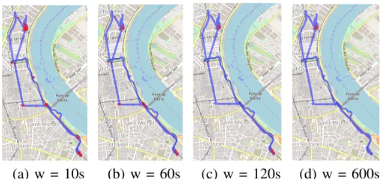
abso-(a) w = 10s (b) w = 60s (c) w = 120s (d) w = 600s
Fig. 4. GPS trace (in blue) of a user and her detected stop locations (in red) using our sliding window heuristic, for different window sizes. Figure best viewed in colors.
lute T-statistic3, and (ii) the normalized Euclidean distance between vectors of static session counts in bins of 200 seconds. The results are summarized in the heatmaps of Fig. 3(b)-(c), for the two metrics respectively. It is apparent that the two metrics – despite their inherent differences – return consistent results. Specifically, there are four principal regions of w values that detect very similar static sessions: (i) window sizes below 10 seconds; (ii) window sizes between 10 and 60 seconds; (iii) window sizes between 60 and 120 seconds; and, (iv) window sizes above 120 seconds.
We provide an example of how these four regions translate into different patterns of detected static sessions in Fig. 4. Each plot refers to a different w value, lying in each of the aforementioned regions, and shows a same target trajectory (in blue) with highlighted stop locations (in red). Clearly, the smaller window sizes result in a larger number of short pauses, seemingly corresponding to short waits at road intersections. As the size of the window increases, these less significant pauses disappear and we are left with the more significant breaks of the mobility. In the last region, for w > 120 seconds, only one long stop location is detected.
Building upon these results, we select a window size w = 60 seconds for the rest of our analysis. This is the smallest (hence more accurate) value that avoids capturing micro-pauses, and that preserves the full duration of important stays at stop locations. Fig. 3(a) highlights in blue the CDF
3Cases with p-value below the significance level 0.05 have been set to the
maximum distance value. This corresponds to a white color code in Fig. 3(b), implying that not enough samples are available to derive a conclusive result under this pairwise difference metric.
(a) (b)
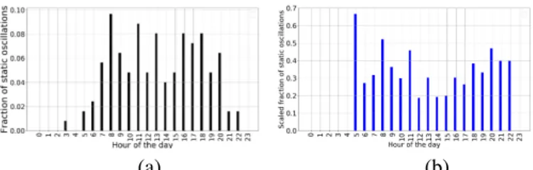
Fig. 5. (a) Fraction of static sessions extracted per hour of the day. (b) Scaled fraction of static sessions with oscillations per hour of the day.
for this window size. By using this w value, we extracted over 1,200 static sessions and more than 3,000 mobile sessions.
C. Occurrence of oscillation patterns in static sessions We now study the factors that affect the emergence of oscillations in mobile phone location data, during the static sessions detected from the GPS trajectories. In particular, we consider the impact of the time of the day, the size of the coverage area of the main base station, the density, and the land use of the area where the main base station is located.
As highlighted by the blue curve in Fig. 3(a), more than 80% of the extracted static sessions have durations of at most 4,000 seconds, i.e., little more than one hour. This observation let us associate sessions to specific hours of the day, and analyse the effect of daytime on the oscillation phenomenon. Fig. 5(a) shows the fraction of static sessions at each hour of the day, with respect to the total number of extracted static sessions. We observe peaks of immobility in the early morning and early evening hours and around lunch time. Fig. 5(b) depicts instead the scaled fraction4of static sessions that yield
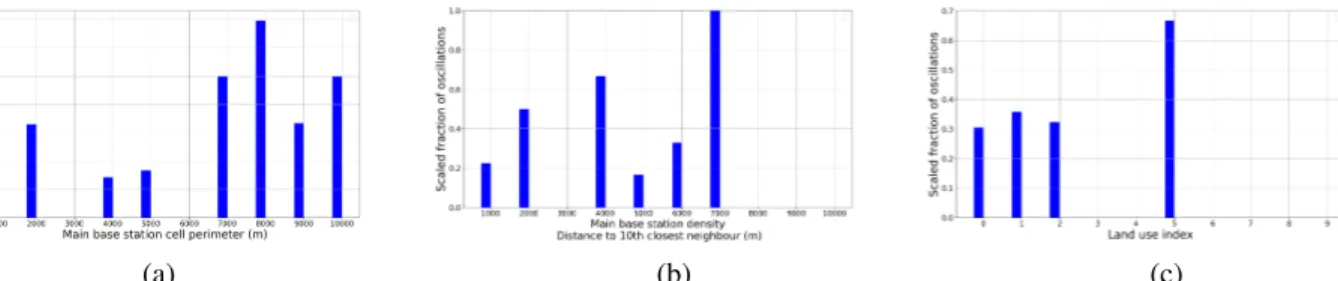
oscillation patterns, per hour of the day. We observe a large fraction in the morning rush hours as well as in the evening. These figures suggest that oscillations in absence of mobility are more likely to appear in rush hours, especially in the early morning and evening, and are less frequent during work hours. As we focus on static sessions, there is one prevalent base station in each such session, appearing more frequently or for the most time. This is the main base station, or station A, in an AXA pattern. Fig. 6(a) shows the fraction of static sessions with oscillation patterns involving a main base station with a particular coverage5, scaled with regards to the total number of static sessions involving main base stations with similar coverage. Quite unsurprisingly, the probability of oscillation is the highest in wide cells with perimeters of 7-10 km, where it reaches values up to 70%: the poor signal quality at the (vast) boundaries of these cells is the likely reason. High chances of oscillations, above 30%, are also recorded in small cells, probably due to the vicinity of other base stations that present reasonable network attachment options for the mobile device. Fig. 6(b) shows instead the scaled fraction of static sessions with oscillations occurring at main base stations located in areas with different mobile network density6. There seems to
be some correlation between the occurrence of oscillations and
4This is computed by counting the number of static sessions occurring at
a given hour of the day during which at least one oscillation pattern exists. We divide by the total number of static sessions recorded during that hour.
5We use the base station Voronoi cell perimeter as a proxy for coverage. 6We consider the distance of the base station from its 10-th nearest
neighbour as an indicator of the density of the radio access infrastructure.
the fact that the main base station is located in an area where the network deployment is sparse. However, the trend is not always consistent, and it is hard to draw conclusions here.
Finally, in Fig. 6(c) we show the scaled fraction of static sessions with oscillations in terms of the land use of the area where the main base station is located. Interestingly, we observe a high chance of oscillations above 70% in the case of congested roadways (land use 5).
D. Occurrence ofAXA patterns in mobile phone locations After analysing oscillations in static sessions of human movement, we take a deeper look into the existing AXA patterns and characterize them in terms of the hour of the day when they occur and the features of the involved base stations. Notice that, so far, we have characterized oscillations in static sessions, whereas now we look at AXA patterns in a general way. This allows investigating the occurrence of oscillations, either during static or mobile sessions.
In order to decide whether a detected AXA pattern corre-sponds to an actual movement or to an oscillation in absence of mobility, we rely on the GPS data. Whenever we encounter an AXA pattern (following Def. 1) in mobile phone location data, we look for the corresponding segment in the GPS trajectory of the same user. If the conditions set by Def. 2 are met during that trajectory segment, then the oscillation is considered to occur during a static session. Otherwise, the user is considered mobile. An issue to address is the choice of the temporal threshold θ in Def. 1, which expresses the duration of a pattern that may be considered as a candidate oscillation. We tested a large number of values, from 5 seconds to approximately 40 hours. In Fig. 7(a) we show the number of detected patterns for different temporal thresholds. We show this for |X| = {1, 2, 3}, as for values |X| > 3 no AXA patterns were detected under any of the temporal thresholds considered. Fig. 7(b) shows instead the fraction of the number of patterns characterized as mobile over those characterized as static, as the temporal threshold θ increases. In both plots, the trends become constant beyond θ = 300 seconds, implying that such a threshold is sufficient to capture the vast majority of the observable patterns. Therefore, we choose θ = 300 seconds for our further analysis, and investigate how different system features affect the probability of occurrence of AXA patterns during static and mobile sessions.
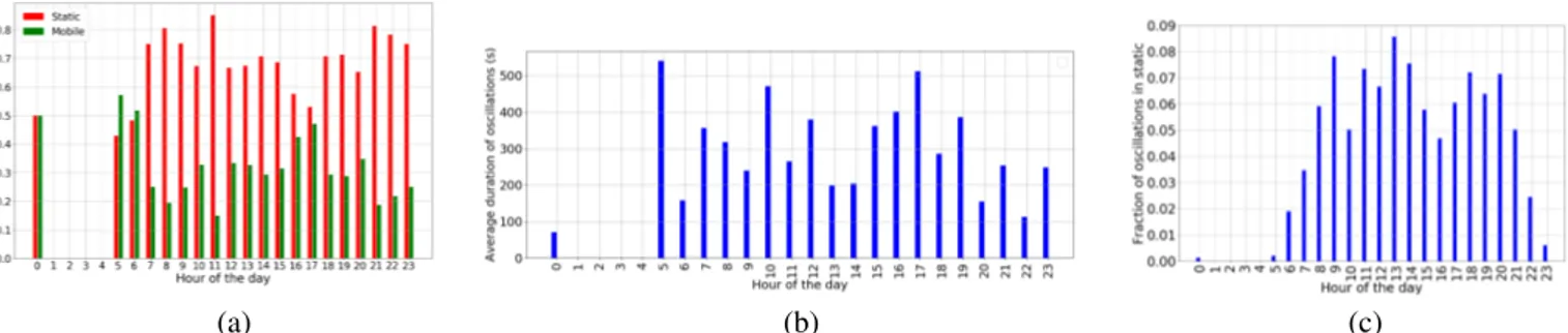
Fig. 8(a) shows the fractions of AXA patterns characterized as static and mobile per hour of the day and highlights how slightly more mobile patterns appear in the early morning rush hours. Fig. 8(b) shows the average duration of an AXA pattern, either during static or mobile sessions, separated based on the hour of the day when those appear. Interestingly, the longest patterns coincide with the hour of the day when we have more mobile patterns – and therefore, actual movement of a user. Fig. 8(c) shows the fraction of AXA patterns in static sessions per hour of the day, across the detected patterns in our database. This exhibits a mixture of normal distributions, centered in the rush hours of the morning, around noon and in the early and late evening, very similar to Fig. 3(b). By looking at the three plots jointly, we conclude that the highest chances of observing an oscillation phenomenon in absence of mobility is during rush hours, where the majority of people either
(a) (b) (c)
Fig. 6. Scaled fraction of static sessions with oscillations over the total number of static sessions: (a) per size of coverage area of main base station, (b) per density area of the main base station, (c) per land use of the area of the main base station.
(a) (b)
Fig. 7. (a) Number of patterns detected for the various temporal thresholds (b) Fraction of number of mobile over static AXA patterns found for the various temporal thresholds.
commute (and therefore get stuck in traffic), or concentrate at shops and transportation hubs.
We also explore how the fraction of detected patterns in static and mobile states varies based on the characteristics of the main base stations7. Fig. 9(a) shows the fraction of AXA patterns appearing during static sessions and that of the same sequences observed in mobile sessions, as the coverage of the base station varies. In all cases, the vast majority of detected patterns correspond to oscillations in static mobility, with these being uniformly distributed across the different base station cell sizes. In Fig. 9(b) we present the fractions of detected AXA patterns in static and mobile conditions, versus the surrounding network density. For the small and medium density cases, the vast majority of found patterns are oscillations while the user is still: this further supports that it is more probable to observe such a phenomenon when static in a dense area with many visible surrounding base stations. Conversely, in the cases of the base stations that are located in the sparser areas, the majority of the patterns correspond to actual mobility. Finally, in Fig. 9(c) we show the fraction of static and mobile AXA patterns with respect to the land use of the area where the main base station is located (see Fig. 1(d)). Here we observe again mostly oscillations in static mode throughout the different categories of land use.
Overall, the previous analyses unveil that no clear-cut rules exist in the appearance of oscillations in absence of mobility with respect to the hour of the day, or to the features of the involved base stations. We found, nonetheless, certain trends as well as the probabilities at which detected patterns can belong to static or mobile status of the tracked user, which we employ in the design of our oscillation filtering technique, next.
7We also investigated similar features for the X base stations, with very
similar results. The associated plots are omitted for the sake of brevity.
IV. TWO APPROACHES TO OSCILLATION FILTERING
Our ultimate goal is to provide a method for the detection and filtering of oscillations in absence of mobility from mobile phone location data. The main challenge here is that we cannot anymore rely on the GPS for the classification of the patterns as mobile or static. For us, GPS data act as auxiliary information that we use at a training, preprocessing step in order to label AXA patterns as oscillations in absence of mobility or actual movement. This step does not have to be applied on the corresponding GPS traces of the mobile phone location data that we wish to filter from oscillations and can be performed solely one-off for the base stations of a region. To this end, we propose a two-phases approach. During the first phase, we detect AXA patterns in mobile phone location data and classify them as mobile or static. During the second phase, we filter the oscillations from the detected static patterns (i.e., the oscillations we found occurring while the user is static). Next, we detail the phases of our methodology.
A. Detection and classification of patterns
In this first phase of our methodology, we wish to classify a detected AXA pattern as mobility or oscillation in absence of mobility. We propose two classification techniques: (i) a probabilistic one and (ii) one based on machine learning. Probabilistic classification. We compute the probabilities of a detected pattern being an oscillation in absence of mobility or actual movement, given a particular time of the day or specific features of the main base station, from 80% of randomly selected traces in our dataset, as per Figures 8(a) and 9(a)-(c). Specifically, for static AXA patterns, we have
p(st) =Y
y
p(st_y_i), (1) where p(st_y_i) is the probability of the base station i in the detected AXA pattern to be involved in a static oscillation and y could either correspond to the hour of the day, the perimeter of the coverage area of the base station, its density or its land use. An equivalent expression holds for the probability p(mo) of AXA patterns to represent actual movement.
We then classify every detected pattern as static or mobile according to the highest computed probability between p(st) and p(mo). The performance of this approach is tested on patterns detected in the remaining 20% of our dataset. Machine learning classification. We employ a decision tree that uses the time of the day of the detected pattern and the involved base station features as conditions, and labels every
(a) (b) (c)
Fig. 8. (a) Fraction of patterns appearing in static or mobile state at different times of the day (b) Average duration of detected patterns per time of the day (c) Fraction of detected AXA oscillation patterns in static state per time of the day.
(a) (b) (c)
Fig. 9. (a) Fraction of patterns appearing at main base stations of different sizes (b) Fraction of patterns appearing given the density of the main base station (c) Fraction of patterns appearing given the land use of the area where the main base station is located.
pattern as mobile or static. We cross-validated our results, using 80% of traces in our dataset as training population and the remaining 20% for testing. We run this experiment independently 100 times and show here the aggregated results. During training, for every extracted AXA pattern from the mobile phone data, we extract the corresponding segment from the GPS data and, based on its radius of gyration and its average instant speed, we classify it as static or mobile. Along with the label, we store the hour of the day and the features of the base stations of the pattern.
Evaluation. We evaluate the two approaches by computing (a) the accuracy of the classification (that is, if we correctly label a pattern as static or mobile) and (b) the recall of the classification (that is, if we detect and correctly classify as static all existing static AXA patterns). For the evaluation, we construct the ground truth using the GPS data, using the methodology described in the previous sections, and compare with the classification of the probabilistic approach or that of the decision tree directly on the mobile phone data. Table I shows the results we obtain, when all features are taken into account. The highest accuracy is obtained when we employ a decision tree. In this case, we obtain accuracy of 87% on average, and 90% at most. For the probabilistic method the accuracy is just slightly lower. For the sake of completeness, we mention that the results are similar or slightly worse, for both methods, when the features are taken individually. In terms of recall, the probabilistic method performs almost impeccably, with the decision tree following very close. B. Filtering of oscillations
Being confident that our methods detect and classify cor-rectly most instances of oscillation patterns in absence of
Approach Accuracy Recall Probabilistic 86% 99% Decision Tree 87% (max: 90%) 97%
TABLE I. Accuracy and recall of AXA pattern classification approaches.
(a) (b)
Fig. 10. (a) Percentage of removed oscillations in absence of mobility. (b) PDF of the error metric between the filtered mobile phone trajectories and the ground-truth GPS ones.
mobility, we proceed to their removal from the mobile phone location data. We wish to filter as many oscillations as possible when the user is static, while preserving the AXA patterns if those correspond to actual mobility. The principle we employ to this end is simple: whenever an AXA pattern is found in the mobile phone location data and our classifier labels that as static, we replace the in-stances corresponding to the oscillation-produced base sta-tion(s) X with the main one A, maintaining though the original timestamps of all records. For instance, let T = {(bsA, t0), (bsX, t1), (bsA, t2)} be a detected AXA pattern
classified as static. Our filter will replace T with the trajectory segment T0= {(bsA, t0), (bsA, t1), (bsA, t2)}.
Evaluation. We evaluate our approach by counting the number of oscillations in absence of mobility before and after the
application of the filtering method. We look both at the case where we classify the detected patterns using the probabilistic approach and the decision tree. We compare our techniques with the state-of-the-art in filtering mobile phone location data from oscillations and noise, i.e. the recursive look-ahead filter (LAF) [9]. The LAF was configured with speed thresholds at 100m/s and 200m/s, which are commonly adopted in the literature, and at 1.5m/s, for a fairer comparison with the settings in our proposed methods. Fig. 10(a) summarizes the results. Our techniques remove almost all oscillations in ab-sence of mobility, under both probabilistic (97%) and decision tree (95%). The LAF, on the other hand, cannot remove the majority of oscillating patterns (removed oscillations stay at 20-30% of the total), and requires a very low speed threshold in order to achieve a 80% figure. We highlight that, although LAF is perhaps a better choice in removing noisy jumps in mobile segments of a user’s trajectory, this technique is not sufficient to remove the annoying phenomenon that causes a user to seem mobile while she is in fact static.
In order to further assess the quality of the filtering ap-proaches, we design the following experiment. We define an error metric that estimates whether after the filtering of a mobile phone data trajectory, its distance to the corresponding GPS trajectory has increased or decreased. Namely, we com-pute the Hausdorff distance between a GPS trajectory and the corresponding mobile phone location data before (denoted by Hbef) and after (Haf t) the filtering, and compute our error
metric as Hbef − Haf t, normalizing the values in the range
[−1, 1]. Here, a value −1 indicates a maximally increased distance, hence a negative result implies that the filtering process shifts the mobile phone trajectory away from the ground-truth GPS trajectory. Instead, a value of 1 maps to a maximum reduction of the distance between the filtered mobile phone trajectory and the GPS one.
As we can appreciate in Fig. 10(b), the PDF of such an error metric when using the LFA is typically negative, as the LFA does not filter the oscillations, and risks to pick incorrect base stations (i.e., those in X) when it recognizes the AXA patterns. Instead, our techniques exhibit better performance. In particular, with our probabilistic filtering technique, the error metric values become largely positive, indicating that the quality of the filtered trajectory is improved significantly.
V. RELATEDWORK
Stop locations. Different methodologies can be designed for the different sources of location data, including the likes of Wi-Fi access point sequences, CDR data, GPS records, etc.
There are two main methodologies for detecting stop loca-tions in GPS traces. Among the first works for processing trajectory data, [8] uses two scale parameters, namely the roaming distance and the stay duration, accounting for the maximum distance an object can stray from a point location and the minimum duration an object can stay within roaming distance to qualify as stop location, respectively. Although in our approach we do account for similar features, we avoid hard temporal thresholds and rather consider thresholds on the instant speed of the user, as a good indicator of her mobility status. A more recent work [21] uses kernel density for the detection of stop locations in GPS streams. This approach
takes a global view of the location dataset, where the local density maxima are the candidates for stop locations.
GPS data has also been used to characterize mobility as sequences of movement and stops [4]. A set of metrics includ-ing radius of gyration, standard deviation of displacement and total covered distance was employed to represent aggregated information about the movement of a tracked user and was considered suitable for detecting stop locations as well. The main focus in [4] is to spatially characterize appearance of depression in mobile users and, therefore, no evaluation on the detection or identification of stops is provided. Places of interest are identified in [7] using a temporal threshold of 6 hours of non mobility. However, the focus of that work is the privacy concerns rising from spatiotemporal data.
Some researches have employed mobile phone location data [3], [10], [19]. Calabrese et al. [3] are estimating origin-destination flows from mobile phone location data and detect changes of locations where users stop for as low as 1.5 hours. Hoteit et al. [10] study the bias of call detail records in inferring stops or points of interest. The focus of the work is to complete CDR data and not the detection of points of interest per se. Finally, in [19], the authors wish to use longterm GSM data for the detection of frequent stop locations. However, they use GPS data and hard thresholds for the detection of stops and then correlate those with CDR data.
Oscillation phenomenon. Recent works in literature have attempted to firstly define the oscillation phenomenon and then suggest methods to detect and correct it [1], [5], [11], [14], [23], [24]. Existing definitions are not formal, but they all converge in context. In essence, the definitions are similar to the one we propose. However, ours is especially conceived for the cases when the tracked users are static.
Closer to our approach are methods that define particular patterns and take into account the time information. [23] proposes two methods, namely circular and pattern-based. In the circular case, an oscillation is defined as an AXA pattern, where X 6= A and |X| >= 1, and the temporal window is set at 5 minutes, after trial and error, arguing that longer time windows might consider actual mobile trips. The pattern-based case detects oscillations of the ABAB type with the added condition that only one of the consecutive intervals is less than 5 minutes. Such pattern describes small scale movement and would actually correspond to the user being mobile. [14], [24] take a similar approach: they look for suspicious sequences that contain circular events within a short time. Whereas Wu et al., [24] consider time windows of 1 minute, Qi et al., [14] try a few combinations of time intervals and distance thresholds. Similar approaches have been proposed in [1], [12], [20]. Bayir et al. [1] also consider the case of triple switches. Their approach was designed for a particular dataset, which requested users to semantically tag their visited locations. The same dataset was used by [20]. The methods proposed in these two works are not applicable to datasets without semantic tag. The speed between switches has been considered in [11]. A switching sequence is defined as oscillation if the switching speed exceeds 200km/h. Their definition is further extended to account for the difference in the heading directions between two consecutive displacements, which should be set at 180 degrees. As argued in [5], the speed criterion is not always
reliable by itself, given the low accuracy of location estimation in CDR data and the small time intervals between switches.
In [17], Rodriguez-Carrion et al. investigate the presence of biases in human mobility analyses based on CDR. As a preliminary step to the study, they preprocess mobile phone location datasets so as to remove oscillations. Specifically, oscillations are detected as simple AXA sequences, where X can include either one or two base stations; the definition is time-agnostic, and the AXA pattern can span any time interval. Then, three different techniques are used to remove the oscillation, using (i) the most frequent base station, (ii) the base station A that bounds the patterns, or (iii) a combination of the two. Similarly, Wu et al. [24] propose to replace sequences of oscillations by the base station that appears most frequently and has the smaller average distance from all other base stations, in the oscillation sequence. However, in all these solutions, only the spatial dimension of the oscillation is considered. Our work removes such a limitation, by detecting and correcting oscillations in both space and time.
VI. CONCLUSIVE REMARKS
We presented a comprehensive analysis of the oscillation phenomenon in static instances of human mobility and char-acterized it in terms of the hour of the day it occurs and features of the base stations involved in it. We proposed next a method to filter out such occurrences from mobile phone location data. Our method first classifies detected occurrences as actual mobility or oscillation phenomenon by using either a probabilistic method or a decision tree. Our filtering technique removes almost all existing oscillations in absence of mobility and outperforms the state of the art look-ahead filter technique. A user-centric analysis, on the basis of a larger and more diverse dataset, as well as the investigation of using more machine learning techniques, are left as future work.
ACKNOWLEDGMENTS
This work was partially supported by the ANR CANCAN 18-CE25-0011) and the ANR PROMENADE (ANR-18-CE22-0008) projects.
REFERENCES
[1] M. A. Bayir, M. Demirbas, and N. Eagle. Mobility profiler: A frame-work for discovering mobility profiles of cell phone users. Pervasive and Mobile Computing, 6(4):435 – 454, 2010. Human Behavior in Ubiquitous Environments: Modeling of Human Mobility Patterns. [2] V. D. Blondel, A. Decuyper, and G. Krings. A survey of results on
mobile phone datasets analysis. EPJ Data Science, 4(1), Aug 2015. [3] F. Calabrese, G. Di Lorenzo, L. Liu, and C. Ratti. Estimating
origin-destination flows using opportunistically collected mobile phone location data from one million users in boston metropolitan area. IEEE Pervasive Computing, 10(4):36–44, 2011.
[4] L. Canzian and M. Musolesi. Trajectories of depression: unobtrusive monitoring of depressive states by means of smartphone mobility traces analysis. In Proceedings of the 2015 ACM international joint conference on pervasive and ubiquitous computing. ACM, 2015.
[5] M. G. Demissie, G. H. de Almeida Correia, and C. Bento. Intelligent road traffic status detection system through cellular networks handover information: An exploratory study. Transportation research part C: emerging technologies, 32:76–88, 2013.
[6] A. Furno, M. Fiore, R. Stanica, C. Ziemlicki, and Z. Smoreda. A tale of ten cities: Characterizing signatures of mobile traffic in urban areas. IEEE Transactions on Mobile Computing, 16(10):2682–2696, 2017.
[7] S. Gambs, M.-O. Killijian, and M. N. del Prado Cortez. Show me how you move and i will tell you who you are. In Proceedings of the 3rd ACM SIGSPATIAL International Workshop on Security and Privacy in GIS and LBS, pages 34–41. ACM, 2010.
[8] R. Hariharan and K. Toyama. Project lachesis: parsing and modeling lo-cation histories. In International Conference on Geographic Information Science. Springer, 2004.
[9] C. Horn, S. Klampfl, M. Cik, and T. Reiter. Detecting outliers in cell phone data: correcting trajectories to improve traffic modeling. Trans-portation Research Record: Journal of the TransTrans-portation Research Board, (2405):49–56, 2014.
[10] S. Hoteit, G. Chen, A. Viana, and M. Fiore. Filling the gaps: On the completion of sparse call detail records for mobility analysis. In Proceedings of the Eleventh ACM Workshop on Challenged Networks, pages 45–50. ACM, 2016.
[11] C. Iovan, A.-M. Olteanu-Raimond, T. Couronné, and Z. Smoreda. Moving and calling: Mobile phone data quality measurements and spatiotemporal uncertainty in human mobility studies. In Geographic information science at the heart of Europe. Springer, 2013.
[12] J.-K. Lee and J. C. Hou. Modeling steady-state and transient behaviors of user mobility: formulation, analysis, and application. In Proceedings of the 7th ACM international symposium on Mobile ad hoc networking and computing, pages 85–96. ACM, 2006.
[13] D. Naboulsi, M. Fiore, S. Ribot, and R. Stanica. Large-scale mobile traffic analysis: a survey. IEEE Communications Surveys and Tutorials, 18(1), 2016.
[14] L. Qi, Y. Qiao, F. B. Abdesslem, Z. Ma, and J. Yang. Oscillation resolution for massive cell phone traffic data. In Proceedings of the First Workshop on Mobile Data, MobiData ’16, pages 25–30, New York, NY, USA, 2016. ACM.
[15] Y. Qi, C. Yu, Y.-J. Suh, and S. Y. Jang. Gps tethering for energy conservation. In Wireless Communications and Networking Conference (WCNC), 2015 IEEE, pages 1320–1325. IEEE, 2015.
[16] S. Reddy, M. Mun, J. Burke, D. Estrin, M. Hansen, and M. Srivas-tava. Using mobile phones to determine transportation modes. ACM Transactions on Sensor Networks (TOSN), 6(2):13, 2010.
[17] A. Rodriguez-Carrion, C. Garcia-Rubio, and C. Campo. Detecting and reducing biases in cellular-based mobility data sets. Entropy, 20(10):736, 2018.
[18] C. Schneider, V. Belik, T. Couronne, Z. Smoreda, and M. Gonzalez. Unravelling daily human mobility motifs. Interface, 10(84), 2013. [19] D. Schulz, S. Bothe, and C. Körner. Human mobility from gsm data-a
valid alternative to gps. In Mobile data challenge 2012 workshop, June, 2012.
[20] S. A. Shad and E. Chen. Cell oscillation resolution in mobility profile building. CoRR, abs/1206.5795, 2012.
[21] B. Thierry, B. Chaix, and Y. Kestens. Detecting activity locations from raw gps data: a novel kernel-based algorithm. International journal of health geographics, 12(1), 2013.
[22] S. Vanini, F. Faraci, A. Ferrari, and S. Giordano. Using barometric pres-sure data to recognize vertical displacement activities on smartphones. Computer Communications, 87:37–48, 2016.
[23] F. Wang and C. Chen. On data processing required to derive mobility patterns from passively-generated mobile phone data. Transportation Research Part C: Emerging Technologies, 87:58 – 74, 2018.
[24] W. Wu, Y. Wang, J. B. Gomes, S. Antonatos, M. Xue, P. Yang, G. E. Yap, X. Li, S. Krishnaswamy, J. Decraene, et al. Oscillation resolution for mobile phone cellular tower data to enable mobility modelling. In Mobile Data Management (MDM), 2014 IEEE 15th International Conference on, volume 1, pages 321–328. IEEE, 2014.
[25] Y. Zheng. Trajectory data mining: An overview. ACM Trans. Intell. Syst. Technol., 6(3), May 2015.
[26] Y. Zheng, Y. Chen, Q. Li, X. Xie, and W.-Y. Ma. Understanding transportation modes based on gps data for web applications. ACM Transactions on the Web (TWEB), 4(1):1, 2010.