HAL Id: hal-01202028
https://hal.archives-ouvertes.fr/hal-01202028
Submitted on 30 Sep 2015
HAL is a multi-disciplinary open access
archive for the deposit and dissemination of
sci-entific research documents, whether they are
pub-lished or not. The documents may come from
teaching and research institutions in France or
abroad, or from public or private research centers.
L’archive ouverte pluridisciplinaire HAL, est
destinée au dépôt et à la diffusion de documents
scientifiques de niveau recherche, publiés ou non,
émanant des établissements d’enseignement et de
recherche français ou étrangers, des laboratoires
publics ou privés.
Rejection-based classification for action recognition
using a spatio-temporal dictionary
Stefen Chan Wai Tim, Michèle Rombaut, Denis Pellerin
To cite this version:
Stefen Chan Wai Tim, Michèle Rombaut, Denis Pellerin. Rejection-based classification for action
recognition using a spatio-temporal dictionary. EUSIPCO 2015 - 23th European Signal Processing
Conference, Aug 2015, Nice, France. �hal-01202028�
REJECTION-BASED CLASSIFICATION FOR ACTION RECOGNITION USING A
SPATIO-TEMPORAL DICTIONARY
Stefen Chan Wai Tim, Michele Rombaut, Denis Pellerin
Univ. Grenoble Alpes, GIPSA-Lab, F-38000 Grenoble, France
ABSTRACT
This paper presents a method for human action recognition in videos which learns a dictionary whose atoms are spatio-temporal patches. We use these gray-level spatio-spatio-temporal patches to learn motion patterns inside the videos. This method also relies on a part-based human detector in or-der to segment and narrow down several interesting regions inside the videos without a need for bounding boxes annota-tions. We show that the utilization of these parts improves the classification performance. We introduce a rejection-based classification method which is based on a Support Vector Machine. This method has been tested on UCF sports action dataset with good results.
Index Terms— Dictionary Learning, Action Recogni-tion, ClassificaRecogni-tion, Videos, Spatio-temporal patches
1. INTRODUCTION
The research on action recognition has developed a lot in the last years along with the rise of video contents, especially because its applications are numerous in surveillance, auto-matic video annotations or entertainment. Generally, it con-sists in extracting features either globally (or in successive frames) [1, 2] or locally [3]. The goal is to classify some hu-man activities using the data extracted from videos.
Techniques based on dictionaries and sparse representa-tions [4–6] have emerged in action recognition because of the possibility to represent complex patterns using a few nary elements. These methods rely on the creation of a dictio-nary which can encode effectively the information contained in an image.
In this paper, we propose a method for human action recognition in the context of gray-level video sequences. This method learns a dictionary of spatio-temporal atoms coupled with a part-based human detector to select interesting spatio-temporal regions inside a video. We also introduce an original three-stepped rejection-based classification method based on a SVM in order to improve the results. The paper is organized as follows: Section 2 presents the proposed action
This work has been partially supported by the LabEx PERSYVAL-Lab (ANR-11-LABX-0025).
recognition method, Section 3 describes the results obtained and Section 4 presents the conclusions.
2. METHOD FRAMEWORK
The proposed method consists in classifying temporal blocks composed of several frames and containing a human who per-foms one particular action which corresponds to a class.
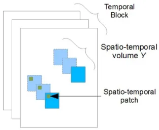
We call temporal block t successive frames of a video. In these blocks, we define spatio-temporal volumes which corre-spond to the same spatial regions taken in successive frames inside the videos. These spatio-temporal volumes are local-ized around areas of interest. Spatio-temporal volumes them-selves are composed of small spatio-temporal patches which are defined as a succession of spatial image patches (see Fig-ure 1). A dictionary is a learned collection of such patches called atoms.
Fig. 1. Example of a temporal block of t = 3 frames described with 2 spatio-temporal volumes. Each volume is composed of a collection of small spatio-temporal patches.
The method described below is based on a previous work [7] and relies on a spatio-temporal patch-based dictionary to represent spatio-temporal volumes. In this paper, we also use a part-based human representation to narrow down the image
to interesting regions. This method is described in 3 parts: (i) Dictionary learning, (ii) Spatio-temporal objects and (iii) Classification with rejection.
2.1. Dictionary Learning
At first, dictionary learning methods were used for denois-ing and inpaintdenois-ing [8, 9] and now, different methods exist in the literature to learn dictionaries for sparse representa-tions. Some of them are specifically designed for classifica-tion, for example DKSVD [10] or GDDL [11]. Dictionary-based methods got great success, in particular, in face recog-nition applications. However, these methods are often appli-cation specific and cannot be straightforwardly used in action recognition because they rely on the alignment of the images. We want to learn a dictionary on spatio-temporal patches in order to describe movement patterns. We cannot utilize large patches and learn a dictionary that can efficiently dis-criminate between the different classes because the actions are complex and we cannot align these images. As a conse-quence, we are using small patches compared to the spatio-temporal volumes. Since the patches are small compared to the complexity of the data, there may be no specific or dis-criminative atoms for each class (different classes may utilize similar atoms) and the recognition is done solely on the pro-portion of used atoms. That is why we chose to implement K-SVD [9] for learning the dictionary.
Let p be a spatio-temporal gray-level patch of size (s × s × t), with s being the size of a square patch in the spatial di-mensions and t being the number of frames considered in the temporal dimension. The patch pnormis the patch p whose set of pixels are normalized so that it has zero mean and unit norm.
Let Y = [pnorm,1, pnorm,2, ..., pnorm,m] ∈ Rn×mbe a
a matrix composed of spatio-temporal patches, with m being the size of the dataset, n the dimension of the patches and D = [d1, d2, ..., dNatoms] ∈ R
n×Natoms be the dictionary
of Natoms atoms dk, where the number Natoms is chosen
empirically.
The dictionary learning algorithm K-SVD [9] is an itera-tive algorithm which can solve the optimization problem. The formulation of the dictionary learning algorithm is:
min
D,X{kY − DXk 2
F} such that ∀i ∈ [1, m] , kxik0≤ T0 (1)
where X = [x1, x2, ..., xm] ∈ RNatoms×mcontains the
co-efficients of the decomposition of Y using the dictionary D. xi = (αj)j∈[1,Natoms] is a column vector from X
describ-ing pnorm,iand kxik0is the norm that counts the number of
non-zero entry of the vector. k · kF is the Frobenius norm:
A ∈ Rn×m, kAkF = q Pn i=1 Pm j=1|aij|2. T0is the
maxi-mum of non-zero entries.
This algorithm is performed in two steps: first by opti-mizing the codes X with a fixed dictionary and secondly by optimizing D with respect to X.
The output of this learning step is a dictionary D com-posed of Natoms(Figure 2). Then, we can compute a sparse
representation of a spatio-temporal volume Y based on the dictionary.
t = 1
t = 2 t = 3
Fig. 2. Example of 20 atoms of size (5 × 5 × 3) pixels from a learned dictionary with K-SVD.
2.2. Spatio-temporal objects
Our objective is to classify successive frames (temporal block) of the video. To do that, we propose to select in-teresting regions within the images (see Figure 1) based on the results of a part-based human detection algorithm. 2.2.1. Part-based human detection
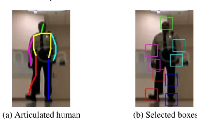
We perform the selection of interesting regions within the images thanks to an existing part-based human detection al-gorithm [12]. The alal-gorithm is based on a deformable parts model capable of handling large variations in the human poses. The output of the algorithm is a list of square bound-ing boxes of fixed size correspondbound-ing to the localizations of the different parts of the model. In the model chosen, the parts are positioned on specific regions of the human body (head, right/left arm, right/left leg ...). The original part-based model contains 26 different parts and we selected only 9 be-cause they approximatively cover the body (Figure 3) and in order to limit the dimension of the block representation (see Section 2.2.2).
From each of the parts, we construct a spatio-temporal volume Y (see Figure 1) by extending the localization of the
parts in the temporal dimension.
(a) Articulated human (b) Selected boxes
Fig. 3. Example of bounding boxes extracted by [12]. (a) is an example of a full part-based human detection. (b) is an example of the 9 parts selected. The images are obtained from a video of the UCF dataset from the class ”Walking”.
2.2.2. Signature computation
We want to classify the human actions represented in videos using the spatio-temporal volumes described in the previous section.
Each volume Y can be described with a histogram: h =
m
X
i=1
xi
with the coefficient vectors xi of all the patches within Y .
Since we are using 9 parts, we can obtain 9 different his-tograms h(j), j = {1, ..9}. The final signature is the con-catenation of the histograms for all of the individual parts: hblock = [h(1), ..., h(j)]. The final dimension of the
signa-ture is Nparts× Natoms.
2.3. Classification with rejection
Once we obtain the signatures for each temporal block, we want to retrieve the action classes for each video. The ex-tracted features consist in signatures obtained for each block of t frames, meaning that, for a video of L frames containing a single action, we can get up to L − t + 1 signatures if we use overlapping blocks of frames. We have developed a method that gives a label to each block. The label of the video is ob-tained by a voting procedure on all the blocks of the video, but since the dimension of the patches and the number of frames t taken into account in each block are small, some signatures may be ambiguous leading to classification errors. That is why we decided to add an extra ”rejection” class which re-groups these ambiguous signatures when training the SVM. Normally, all the signatures extracted from the blocks for the same video share the same label: as a consequence, the objec-tive of this new class is to prevent some signatures that could be ambiguous from voting for a label.
The SVM is trained in three steps.
In the first step, we divide the training set into groups where each group is the set of signatures belonging to a given video of L frames. Indeed, the signatures within the same video normally share a lot of similarities and thus cannot be processed separately. Then we do a leave-one-group-out setup on the training set to optimize the parameters of the SVM.
In the second step, we use the previous leave-one-group-out setup with the optimized parameters and we look for each signature misclassified in each group. The misclassified sig-natures are moved into the ”rejection” class (see Figure 4).
In the third step, a final classifier is learned using all the signatures and all the classes (including the ”rejection” class) as input. The final label for a given video in the test set is obtained by voting using the set of signatures of the videos. Each signature classified in the rejection class is removed from the vote.
We have found that this method can significantly improve the classification results. However, we have to carefully bal-ance the number of elements in the ”rejection” class after the second step. Otherwise, it happens that, during the testing phase, all the signatures of a video can end up classified in the ”rejection” class. We tried different rules for moving an element into the ”rejection” class. The results are presented in Section 3.
(a) One iteration of the leave-one-group-out in the first step. (green = well classified, red = misclassified)
(b) One signature of Video 1 is moved to ”rejection” class D in the second step.
Fig. 4. Example of the second step of the proposed classifica-tion method with 6 videos and 3 classes of acclassifica-tions A, B and C. We use a Leave-one-group-out setup with the signatures of each video as a group. Each signature misclassified during this step goes into the ”rejection” class. At the end of this step, the whole training set (signatures) with the extra class serves to learn the final classifier.
3. EXPERIMENTATIONS
We tested the proposed algorithm of the UCF sports action dataset [13]. This dataset is normally composed of 10 classes: ”Walking”, ”Swinging”, ”Skateboarding”, ”Running”, ”Rid-ing horse”, ”Lift”Rid-ing”, ”Kick”Rid-ing”, ”Play”Rid-ing golf” and ”Div-ing”. The resolution of the videos is (720 × 480) pixels. We decided to remove the class ”Lifting” because of the lack of annotations. In total, we used 9 classes and 140 videos.
For the classification of the videos, we used libLin-ear [14]. We did a leave-one-group-out using all the sig-natures computed for a single video as a group. The size of the patches considered is (5 × 5 × 3) pixels. With the selected temporal size t = 3, we obtained between 20 and 90 signatures for each video depending on its length. Each human was described with 9 volumes of (24 × 24 × 3) pixels computed with the part-based detector. The classification label was determined by votes using all the signatures (or the signatures not classified in the ”rejection” class). Table 1 shows the different performances with and without the use of the part-based detector and the ”rejection” class. We reach 86.4% accuracy with 9 parts and a dictionary D of Natoms = 150 atoms against 72.1% when considering only
one full bounding box including all the body. We chose to take the sparsity T0= 1 for our experiments. In our previous
work, we showed that taking any low value for T0 did not
change the results much but T0 = 1 gave us the best
perfor-mance. The choice of patch size is tied with the dictionary size for overcompleteness. A larger dictionary also leads to larger signature size. Empirically, we found that the choice of (5 × 5 × 3) for the patch size was a good compromise.
We also tried learning a specific dictionary for each indi-vidual part used in our method but the results obtained were the same. Our hypothesis is that the global motion informa-tion of the parts is more important than the local precision in the shape. However, we can also add the precision of the part detection is not perfect for some classes (for example, be-cause of the blur). Moreover, we note that even if many of the boxes are not well-localized, it still improves the classifica-tion performance by a good margin (see Table 1). We believe that, when using a single full bounding box, too many spatial information is lost during the pooling. The fact of using the part detector is a way to reintroduce some spatial information and narrowing down some interesting image regions.
We tried different rules for the ”rejection” class. The first rule tested is to move the misclassified signatures during the first learning step into the ”rejection” class. However, it hap-pened that in some cases, for the test set, all the signatures for a given video could end up rejected meaning that we had to use the classifier learned without our extra class. To prevent that, we tried softer rules: instead of moving all misclassified signatures into the extra class, we only moved signatures with a probability to belong to its true class below a chosen value (see Table 2). These probabilies can be obtained by adding an
Methods Accuracy
Gray-level + Full bounding boxes 72.1% Gray-level + Part-based detector 80.0% Gray-level + Part-based detector 86.4% (SVM with basic ”rejection” class)
Table 1. Performance comparison for our method in different conditions. Dictionary size = 150, Sparsity T0 = 1, video
labels obtained by voting using the signatures of the video.
option in libLinear and are computed using logistic regression for each class. We can see that our extra learning step serves its purpose since the accuracy at signature level jumps from 53.6% to about 80%. Moreover, we can also observe that balancing the ”rejection” class can lead to improved results: going down from 50% rejected signatures to 35% leads to a gain of about 2% in accuracy because of the effects described above.
Rejection rule Video Label Signature % Signatures Accuracy Accuracy rejected
Reference 80.0% 53.6% No Probability 86.4% 87.8% 50.4% Estimates Probability 86.4% 87.5% 38.5% Estimates (Thr: 0.25) Probability 88.6% 85.9% 35.5% Estimates (Thr: 0.15) Probability 87.9% 83.9% 31.2% Estimates (Thr: 0.05)
Table 2. Performance comparison for different rejection rules. Dictionary size = 150, Sparsity T0= 1, video labels obtained
by voting using the signatures of the video. The table gives the video label classification accuracy (obtained after voting), the signature classification accuracy and the proportion of sig-natures rejectedby the classification.
We compare the proposed method with different algo-rithms of the literature in the Table 3. We can see that our method achieves good results. Even if the descriptors ob-tained with the part-based detector alone only reach 80%, the combination of the proposed descriptors and classification method perform really well. The size of the codebook used in our method is 150 compared to 4000 for [15] and 40 for [16] even if the final dimension of the signatures is 1350. Speed wise, the experiments were done on MATLAB so a signifi-cant gain in speed is possible: the part-based human detector was the limiting factor with about 0.5 frame per second on a
modern computer, once the parts are extracted we can com-pute about 7 signatures per second. Results from [17, 18] are given as a comparison: they use techniques different from dictionary-based approach and show that the proposed method is competitive.
Methods Accuracy
Dictionary based methods
H. Wang et al. [15] 85.6% Q. Qiu et al. [16] 83.6% T. Guha et al. [5] 83.8% Proposed method 88.6% Other methods X. Wu et al. [17] 91.3% H. Wang et al. [18] 88.0%
Table 3. Performance comparison for different features and methods for the classification on UCF Sports action dataset. Both dictionary-based and non dictionary-based methods are presented.
4. CONCLUSION
Given a raw video as input, the proposed dictionary-based action recognition method performs efficiently. Despite the small dimension of the patches, we show that using localized spatio-temporal volumes improves the results. We also in-troduced a rejection-based classification method to select the most descriptive signatures to select the labels. The method has been tested on UCF sports action dataset with good re-sults.
For future work, we are looking for a way to take into account the evolution of the signatures extracted from suc-cessive temporal blocks instead of treating them separately. We are also working on more recent databases like UCF50.
REFERENCES
[1] A. A. Efros, A. C. Berg, G. Mori, and J. Malik, “Rec-ognizing action at a distance,” ICCV, 2003.
[2] K. Schindler and L. V. Gool, “Action snippets: How many frames does human action recognition require?,” CVPR, 2008.
[3] P. Scovanner, S. Ali, and M. Shah, “A 3-dimensional sift descriptor and its application to action recognition,” Proceedings of the 15th international conference on Multimedia, 2007.
[4] J. Yang, K. Yu, Y. Gong, and T. Huang, “Linear spatial pyramid matching using sparse coding for image clas-sification,” CVPR, 2009.
[5] T. Guha and R. K. Ward, “Learning sparse representa-tions for human action recognition,” IEEE Transacrepresenta-tions on Pattern Analysis and Machine Intelligence, vol. 34, 2012.
[6] G. Somasundaram, A. Cherian, V. Morellas, and N. Pa-panikolopoulos, “Action recognition using global spatio-temporal features derived from sparse represen-tations,” CVIU, 2013.
[7] S. Chan Wai Tim, M. Rombaut, and D. Pellerin, “Dic-tionary of gray-level 3d patches for action recognition,” in MLSP, 2014.
[8] J. Mairal, F. Bach, J. Ponce, and G. Sapiro, “Online learning for matrix factorization and sparse coding,” Journal of Machine Learning Research, vol. volume 11, pp. pages 19–60, 2010.
[9] M. Aharon, M. Elad, and A. Bruckstein, “K-svd: an algorithm for designing overcomplete dictionaries for sparse representation,” IEEE Transactions on Signal Processing, vol. 54, 2006.
[10] Q. Zhang and B. Li, “Discriminative k-svd for dictio-nary learning in face recognition,” in CVPR, 2010. [11] Y. Suo, M. Dao, U. Srinivas, Vishal Monga, and T. D.
Tran, “Structured dictionary learning for classification,” IEEE Transactions on Signal Processing, 2014. [12] Y. Yang and D. Ramanan, “Articulated human
detec-tion with flexible mixtures of parts,” IEEE Transacdetec-tions on Pattern Analysis and Machine Intelligence, vol. 35, 2013.
[13] M. D. Rodriguez, J. Ahmed, and M. Shah, “Action mach: A spatio-temporal maximum average correlation height filter for action recognition,” in CVPR, 2008. [14] R.-E. Fan, K.-W. Chang, C.-J. Hsieh, X.-R. Wang, and
C.-J. Lin, “Liblinear: A library for large linear classifi-cation,” Journal of Machine Learning Research, vol. 9, 2008.
[15] H. Wang, M. M. Ullah, A. Klaser, I. Laptev, and C. Schmid, “Evaluation of local spatio-temporal fea-tures for action recognition,” British Machine Vision Conference, 2009.
[16] Q. Qiu, Z. Jiang, and R. Chellappa, “Sparse dictionary-based representation and recognition of action at-tributes,” ICCV, 2011.
[17] X. Wu, D. Xu, L. Duan, and J. Luo, “Action recognition using context and appearance distribution features,” in CVPR, 2010.
[18] H. Wang, A. Klaser, C. Schmid, and C-L. Liu, “Dense trajectories and motion boundary descriptors for action recognition,” in IJCV, 2013.


![Risiko- & [und] Schutzfaktoren der psychischen Gesundheit humanitärer Einsatzhelfer : eine systematische Literaturübersicht](data:image/gif;base64,R0lGODlhAQABAIAAAP///wAAACH5BAEAAAAALAAAAAABAAEAAAICRAEAOw==)