HPP: a new software for constrained motion planning

HAL Id: hal-01290850

https://hal.archives-ouvertes.fr/hal-01290850v2

Submitted on 2 Aug 2016

HAL is a multi-disciplinary open access

archive for the deposit and dissemination of

sci-entific research documents, whether they are

pub-lished or not. The documents may come from

teaching and research institutions in France or

abroad, or from public or private research centers.

L’archive ouverte pluridisciplinaire HAL, est

destinée au dépôt et à la diffusion de documents

scientifiques de niveau recherche, publiés ou non,

émanant des établissements d’enseignement et de

recherche français ou étrangers, des laboratoires

publics ou privés.

HPP: a new software for constrained motion planning

Joseph Mirabel, Steve Tonneau, Pierre Fernbach, Anna-Kaarina Seppälä,

Mylène Campana, Nicolas Mansard, Florent Lamiraux

To cite this version:

Joseph Mirabel, Steve Tonneau, Pierre Fernbach, Anna-Kaarina Seppälä, Mylène Campana, et al..

HPP: a new software for constrained motion planning. International Conference on Intelligent Robots

and Systems (IROS 2016), Oct 2016, Daejeon, South Korea. �hal-01290850v2�

HPP: a new software for constrained motion planning

Joseph Mirabel

, Steve Tonneau

, Pierre Fernbach

, Anna-Kaarina Sepp¨al¨a

, Myl`ene Campana

,

Nicolas Mansard

and Florent Lamiraux

Abstract— We present HPP, a software designed for com-plex classes of motion planning problems, such as navigation among movable objects, manipulation, contact-rich multiped locomotion, or elastic rods in cluttered environments. HPP is an open-source answer to the lack of a standard framework for these important issues for robotics and graphics communities. HPP adopts a clear object oriented architecture, which makes it easy to implement parts of an existing planning algorithm, or entirely new algorithms. Python bindings and a visualization tool allow for fast problem setting and prototyping: a new algorithm can be implemented in just a few lines of code.

HPP can be used for classic planning problems such as pick and place for mobile robots, but is specifically designed to solve problems where the motion of the robot is con-strained. Examples of behaviors produced by HPP thanks to a generic constraint formulation include: maintaining a relative orientation between bodies, enforcing the static equilibrium of the robot, or automatically inferring that an object must be moved to allow locomotion. Constraints are tied to a custom representation of the kinematic chain, compatible with the Unified Robot Description format (URDF).

To illustrate the possibilities of HPP, we present several recent scientific contributions implemented with HPP, most of which are provided with Python tutorials. HPP aims at being seamlessly integrated within a global robot control loop: Pinocchio, the fast multi-body dynamics library, is currently being integrated in HPP, thus bridging the gap between the planning and control communities.

I. INTRODUCTION

Schwartz and Sharir define the motion planning problem as follows [1]: “Given a body B, and a region bounded

by a collection of “walls”, either find a continuous motion connecting two given positions and orientations of B during which B avoids collision with the walls, or else establish that no such motion exists”. This formulation covers a “collision avoidance” aspect, and a “motion” aspect of the planning, both dependent on the body.

Motion Planning for collision avoidance

Efficient, generic algorithms [2], [3] have been proposed to explore the space of collision-free configurations [4]. The large majority of methods performs a sampling of this space, with the objective to capture its topology in a roadmap, a graph where nodes correspond to configurations of the robot, connected if a collision-free path exists between them.

*This work has been partly supported by the national PSPC-Romeo 2 project, the ERC-ADV project 340050 Actanthrope, the European Commu-nitys Seventh Framework (FP7/2007-2013) under grant agreements 609206 (Factory-In-A-Day project) and 608849 (EUROC project), and the French agency ANR 13-CORD-002-01 (ENTRACTE project).

1

CNRS, LAAS, 7 avenue du colonel Roche, F–31400 Toulouse, France

2

Univ de Toulouse, LAAS, F–31400 Toulouse, France

Efficient implementation of these algorithms exist nowa-days, in the frameworks OMPL [5], OpenRAVE [6], and Kineo CAM [7]. Thanks to them, assembly/disassembly tasks for manipulator arms, trajectory planning and control of wheeled robots, or human ergonomic studies are achieved on a daily-basis in the industry or the academia. These algo-rithms focus on the “collision avoidance” aspect, since the motion is controlled by well-known differential equations.

Constrained Motion planning

Recently, important scientific contributions have been pro-posed for more difficult classes of motion planning problems, where the augmented motion capabilities of the robot come with constraints on the movement.

For instance, multi-contact planning is the problem where an under-actuated multiped robot can only move through the contact forces exerted by its effectors on the environment [8]. Similarly in the problem of Navigation Among Movable Obstacles (NAMO) [9], [10], if a chair lies in front of a door, a robot may have to move it away before crossing the door. The latter problem can be seen as a motion planning problem where the body B is composed of both the chair (not able to move by itself!) and the robot. This formulation can be applied to the problem of manipulation [11], [12].

For a complex system such as a humanoid robot, all the mentioned aspects must be addressed simultaneously within the same framework [13]. For instance, the challenge course of the DARPA Robotics Challenge integrated multi contact planning, manipulation planning and NAMO altogether. One option is to implement ad-hoc planners for each problem, and to try to use them sequentially. However, this separation is problematic. For instance, let us consider two simultaneous tasks, addressed sequentially. A first planner will find a solution to the first task, but the resulting solution might be incompatible with the second task, resulting in a failure. The only open source solution that takes this approach (to our knowledge) is the Choreonoid software [14]. However it only implements a grasp plugin at the moment.

To our knowledge, no existing software chooses the other option, which is to propose a generic formulation for con-strained motion planning, aiming at simplifying program-ming burden, but also at addressing simultaneously all con-straints within the same algorithm, thus avoiding conflicts. The motivation for developing HPP is to propose the first generic and open source implementation of a constraint-based motion planning software.

Contributions and paper structure

HPP is a set of C++ open-source libraries for Linux. The organization of this paper is designed to reflect the rationale between the three main libraries. The first building block is hpp-model. It provides definitions and func-tions for the kinematic model of a robot and the geomet-ric objects of a problem (Section II). The key library is hpp-constraints, a generic constraint framework im-plemented on top of hpp-model (Section III). The motion planning features of HPP are implemented in hpp-core, using a object-oriented architecture that allows customizing parts of a motion planning algorithm in a few lines of C++, or in Python through CORBA bindings (Section IV).

At the end of the paper, we present several cases studies: we compare HPP with OMPL in classic motion planning scenarios, and present several scientific contributions that illustrate the interest of HPP (Section V).

II. KINEMATIC MODEL

Contrary to OMPL, and similarly to OpenRAVE and Choreonoid, HPP commits to a kinematic model. This is justified by the fact that implementing a generic constraint system requires defining the notion of Joint and its asso-ciated joint velocity space, organized in a kinematic tree (or Device). Though it is possible to extend the hpp-model library with custom Joint types and kinematic chains, HPP conveniently handles natively most of the common joints.

URDF files are used for the external representation of the kinematic model, making it compatible with ROS [15].

A. Joint and Kinematic chain implementation

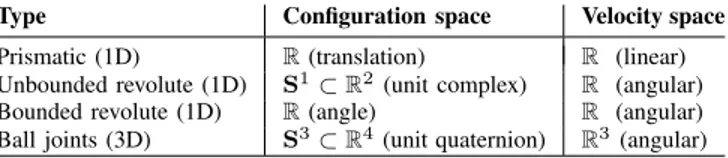
A kinematic chain is implemented as a tree of joints moving inertial and geometrical objects. The configuration space of a robot is the Cartesian product of the configuration spaces of its joints (and possibly of a vector space called ExtraConfigSpace, used for manipulating external ob-jects, and described later). Table I displays the default joint types handled in HPP. Users can also define their own joints. We explicitly and natively handle joints for which the configuration space is a Lie group [16] (e.g. ball joints). For these joints, we use a representation both continuous and robust to singularities (e.g. for ball joints, the space is SO(3), and we use quaternions rather than Euler angles representation). It results that the joint velocity has a smaller dimension than the joint configuration (i.e. the velocity belongs to the Lie Algebra, tangent to the Lie Group).

B. Operations on the configuration space

The configuration of the robot is described by a vector

q ∈ Rn

, where n is the sum of dimensions of each joint,

while the configuration velocity, denoted (abusively) by ˙q,

may have a smaller dimension. Functions are provided to manipulate configuration and velocity vectors:

• integrate(q,˙q) computes the configuration reached

from q after applying velocity ˙q during unit time.

• difference(q1, q2) computes the velocity that leads

from q1 to q2 in unit time.

Type Configuration space Velocity space Prismatic (1D) R (translation) R (linear) Unbounded revolute (1D) S1

⊂_R2(unit complex) R (angular) Bounded revolute (1D) R (angle) R (angular) Ball joints (3D) S3

⊂R4

(unit quaternion) R3

(angular) TABLE I: Main types of joints provided by default. For each joint, we specify the representation of their configuration

space (q vector) and their tangent space (velocity ˙q vector).

These two functions are a generalization of most simple op-erations typically used in motion planning on vector spaces, such as linear interpolation between two configurations.

Geometrical objects are stored using a modified version of FCL [17]. We thus rely on this library for distance and collision computations.

III. DIFFERENTIABLE FUNCTIONS AS CONSTRAINTS The key asset of HPP is the implementation of non-linear constraints as differentiable functions. HPP also provides methods to automatically project a sampled configuration into the configuration space described by the constraint.

OMPL does not handle constraints natively since it does not commit to a kinematic model. Regarding OpenRAVE, and the integration of OMPL with Moveit!, it appears that only positional constraints are handled (inverse kinemat-ics), and mostly limited to manipulator arms. For instance OpenRAVE relies on analytic inverse kinematics methods, which do not apply to chains with more than 6 or 7 degrees of freedom (unless some are disabled). Choreonoid on the other hand also handles static equilibrium and advanced manipulation constraints, in two independent plugins, with no trivial mean to coordinate them.

HPP handles indifferently any constraint that can be written with a differentiable function in a unified way, and proposes several default implementations, including the one proposed by other softwares (see the list below). Any number of constraints can be handled simultaneously.

A. Non-Linear equality and inequality constraints

Differentiable functions can be used by a motion planner to ensure that the configurations of a path (or a subpath) verify one or several constraints. Given a function f that takes its values in a vector space of arbitrary dimension m, a constraint can be defined as:

f(q) = c

where c ∈ Rm

is constant. A user-defined constraint is thus defined by three elements: the function f , the objective value c, and the Jacobian of f . Automatic differentiation is also implemented to spare the need of manually computing the analytical formulation of the Jacobian of f , thanks to a symbolic library. These parameters are used in a Newton’s descent algorithm [18, Alg. 2] to project a given configura-tion on the constraint. This algorithm tends to have better results [19]. The user implements these elements by over-loading the abstract class DifferentiableFunction.

Lf2(f ) Lf1(f ) Lf0(f ) Lg2(g) Lg1(g) Lg0(g)

Fig. 1: Example of level sets of two functions f and g in the configuration space. A global path (blue) is decomposed as elementary paths in each level set. Every elementary path lies in a unique level set. A metaphor is to consider the Lfs(f ) constraints as floors, and the Lgs(g) constraints as

stairs, between which one must alternate to change floors.

Several concrete constraints are implemented in HPP, among which: item orientation and / or position (for inverse kine-matics), relative orientation and / or position of two bodies, static equilibrium, position of the center of mass, distance between bodies, contact between a robot body and a surface. Additionally, HPP can also handle inequality constraints,

written in the form f(q) ≤ c. One motivational example for

inequality constraints is to address a scenario where a robot carries a glass containing a liquid that must not be spilled. This can be expressed by constraining the angle between the glass inclination and to be lesser than a threshold value, and thus be automatically handled by HPP in the planning.

B. Constraint graphs

Furthermore, HPP supports constraint graphs [11]. This representation has the huge advantage of allowing the inte-gration of the discrete, higher-level task scheduling problem into the motion planning problem.

A constraint graph can be seen as a finite state machine, with special nodes and transitions. Each node is characterized by a constraint. The constraint is the level set of a function

f denoted by Lc0(f ) = {q ∈ C|f (q) = c0}. Lc0 is a

submanifold of the configuration space. The submanifolds form a foliation of the configuration space, and intersect in a combinatorial manner. Sampling configurations at the intersection of the submanifolds is required to travel between the level sets. A metaphor for this issue is to consider the problem of going from one floor to another floor of a building, which requires to cross some stairs. Each floor and staircase can be seen as level sets, illustrated in Fig. 1. In general, the probability to sample configurations at the intersection of manifolds is small or null. A constrained motion planner must account for this property and explicitly bias the sampling with projectors (Section III-A).

HPP is provided with an implementation of such algo-rithm, called Manipulation-RRT, presented in details in [20].

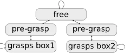
It takes a constraint graph as input, and automatically gener-ates a motion that respects the transition rules of the graph. This formulation can be used to address simultaneously various problems such as quasi-static locomotion (Fig. 2), advanced manipulation (Fig. 3), and even more complex problems, which require multiple manipulations of the same object (such as the Hano¨ı towers game).

At any stage in the resulting path, the configuration of the robot is in one of the states of the graph. For instance, considering the graph in (Fig. 3), the robot is always either: grasping a box, in which case the box is constrained to lie in its hand; not grasping a box, in which case the box is constrained to remain in its previous position; “pre-grasping” a box, in which case the hand of the robot is constrained to be around the non-moving box.

Fig. 2: “Constraint graph” for quasi-static walk on flat ground. Such locomotion requires the Center Of Mass lying above the support polygon defined by the contact points at all times. The difficulty to handle the transition between double and simple support phases is automatically addressed with this constraint graph. DS stands for Double Support, SS for

Single Support, and COML (resp COMR) for the Center Of

Mass lying above the left (resp. right) foot.

Fig. 3: “Constraint graph” for a manipulation scenario in-volving two boxes. The graph is similar to the walking graph. The “pre-graph” constraints correspond to a box being in contact with a surface, with the robot gripper seizing them. From this state the box can be released safely (“free”), or grasped and moved along with the effector (“grasp”).

IV. USINGHPP

HPP can be used either as an off-the shelf motion planner, or as a research tool to implement and test new algorithms. In any case, the main user interactions occur through the

hpp-corelibrary. hpp-core provides methods to set up

the parameters of a motion planning problem, define differ-entiable constraints, and solve the problem. The methods are available either through the C++ API or the Python interface. Additionally benchmarking tools compatible with the OMPL API are provided. Lastly, a unique feature of HPP is the automatic export of computed motion to the Blender [21] animation software for high-quality presentation videos.

A. CORBA Architecture

The client / server CORBA architecture adopted by HPP is an essential asset. It allows to consider integration with other softwares developed in different languages, and distributed execution on robots and computers. HPP is delivered with an exhaustive Python integration through CORBA. C++ algo-rithms can thus be easily called from simpler Python scripts, which allow command line interaction with the software.

Moreover, these bindings are really useful for fast proto-typing and testing new algorithms. Setting up a problem, and even implementing a new motion algorithm, only requires a few lines of code, as shown in the following sections.

B. Setting up and solving a problem

HPP is delivered with tutorials addressing classic or con-strained motion planning, available on the documentation. Code Listing 1 provides an example code for setting up a problem. It shows that the helper class ProblemSolver can be used to customize a problem solver: a single operation is required to change any component of the planning (here, the motion planner type and the path optimization algorithm).

Listing 1: Python code to set up and solve a problem

from hpp.corbaserver.pr2 import Robot robot = Robot ("pr2")

robot.setJointBounds ("base_joint_xy", [-6, -3, -5, -3])

from hpp.corbaserver import ProblemSolver ps = ProblemSolver (robot)

ps.selectPathPlanner("VisibilityPrmPlanner") ps.addPathOptimizer("GradientBased")

# copy the initial configuration

q_init = robot.getCurrentConfig () q_goal = q_init [::]

# ask the robot to move backwards

q_goal [0:2] = [-6, -3]

from hpp.gepetto import Viewer r = Viewer (ps)

# helper function to load the obstacle mesh # into both viewer and problem solver

r.loadObstacleModel ("iai_maps","kitchen_area","kitchen") ps.setInitialConfig (q_init)

ps.addGoalConfig (q_goal) ps.solve ()

C. Adding constraints

A user can set up constraints for a planning problem, either by instanciating an existing constraint type, or by creating its own constraint. Once a constraint is defined, it will automatically be enforced at any point of the path.

Adding a constraint to the problem can be achieved with a single method call. For instance, let us assume that we want the head of the robot to always look at its hand along the motion. Code Listing 2 shows how this can be achieved by defining an orientation constraint between two joints.

Regarding the f(q) = c formulation, here the constant term

c is the desired orientation. The function f returns the hand orientation in the head frame given a robot configuration.

Similarly, if the user defines a constraint graph for the problem, any configuration in the resulting path is guaranteed to be in a state of the constraint graph, and the consecutive

configurations to respect the transition constraints. For in-stance, the robot can be constrained to look at an object, except when the object is in his hand.

Listing 2: Python code to add a constraint to a problem ps = ProblemSolver (robot)

ps.createOrientationConstraint(

"gaze", #constraint name

"head_joint", #name of head joint

"hand_joint", #name of hand joint

[1,0,0,0] #desired hand orientation in head frame

[True,True,True]) #mask describing the constrained axes

D. Testing, benchmarking, and presenting results

In HPP productiveness is enhanced with tools for gener-ating comparative results and demonstrations.

First, HPP is compatible with the benchmarking API of OMPL (although as of today not all features are imple-mented). A Python script can be used to produce the desired output, thus facilitating comparison with other algorithms. We used this API for the benchmarks presented in Section V. Then, HPP is delivered with a viewer based on Open-SceneGraph, the Gepetto viewer (Viewer in Listing 1). The viewer can receive Python command line prompts, and be used via a GUI, for testing problems.

Lastly, HPP includes Python methods to automatically ex-port a computed motion to the open-source Blender software. Entire paths can be exported with a simple method call, and loaded into Blender by executing a Python script. This allows the automatic production of clearer, better looking demonstrations of scientific contributions.

E. Extending HPP

Thanks to the modular architecture of HPP, any part of a motion planning algorithm can be extended and used in a transparent manner with the rest of the framework. Thanks to the CORBA architecture, it is also trivial to implement the Python bindings for new user-defined methods. For prototyping purposes, it is even possible to write a complete motion planning algorithm in a few lines of Python, as is demonstrated with a standard RRT implementation.

V. RESULTS

A. Benchmarks

We compared the performance of the implementation of the RRT-connect algorithm of OMPL and HPP. OMPL proposes other planners, not implemented in HPP. We did not find other benchmarks from other softwares to compare ourselves to. This benchmark shows that the efficiency of the default planner of HPP is comparable to OMPL.

To carry out the comparison, we used the benchmark database provided by OMPL, picking the three problems

solved with RRT-Connect1. To provide a comparison as fair

as possible, we had to take into account implementation details of OMPL and HPP. Firstly, OMPL uses a range parameter, which determines the maximum distance between

1_{In the third scenario (Pipedream-Ring), no mesh of the ring-shaped robot}

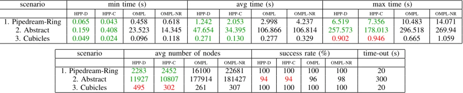
scenario min time (s) avg time (s) max time (s)

HPP-D HPP-C OMPL OMPL-NR HPP-D HPP-C OMPL OMPL-NR HPP-D HPP-C OMPL OMPL-NR

1. Pipedream-Ring 0.065 0.043 0.458 0.618 1.242 2.053 2.998 4.237 6.519 7.356 10.483 14.071 2. Abstract 0.159 0.408 23.523 14.345 47.654 34.395 106.866 106.814 257.573 178.013 296.518 269.94 3. Cubicles 0.049 0.024 0.096 0.118 0.271 0.130 0.277 0.329 0.902 0.946 0.665 1.059

scenario avg number of nodes success rate (%) time-out (s)

HPP-D HPP-C OMPL OMPL-NR HPP-D HPP-C OMPL OMPL-NR

1. Pipedream-Ring 2283 2452 16100 22681 100 100 100 100 20 2. Abstract 11927 10807 177914 181427 94 94 96 98 300

3. Cubicles 495 302 261 307 100 100 100 100 20

TABLE II: Results for 50 runs of each planner. Green values are used when the HPP implementation performs better than all OMPL implementations. Red values are used when HPP performs worse than at least one OMPL implementation. A planning is considered to have failed after running longer than the specified timeout value.

two nodes in the roadmap, automatically computed for each scenario. Depending on the benchmark, this value can improve or slow down the computation time. The HPP implementation does not use such parameter.

Secondly, HPP includes a continuous collision checking method. It has a higher atomic cost than discretized collision checking, but has the advantage that only one test is required between two configurations, regardless of their distance.

To compare HPP and OMPL on an equivalent imple-mentation of RRT-Connect, we consider on one hand a “no range” version of OMPL (OMPL-NR), where the range is set to a high value. On the other hand we consider a HPP implementation with discretized collision checking (HPP-D).

The discretization step is the same in HPP and OMPL2.

To be exhaustive we also included benchmarks performed with the specificities of the softwares: we thus also consider the standard “range” version of OMPL (OMPL), and the continuous collision checking version of HPP (HPP-C).

Table II presents the results for all three scenarios and implementations. The success rate represents the relative number of runs that succeeded before a given maximum time limit. When computing minimum, average and maximum time values, only successful runs were considered. The runs, single-threaded, were performed on a 64 bits computer with 8 processors of 1.2Ghz, 64Go or RAM.

In any considered case, HPP implementation presents equivalent or better average computation times compared to OMPL. The important point is that the performances remain in the same order of magnitude between HPP and OMPL.

B. Use cases

HPP is already actively used for research purposes, some of which are presented here. All the presented projects are open source and accessible to the community on github.com. Most involve constraint-based motion planning, for which HPP is specifically designed, though other applications demonstrate that HPP can be used for classic motion plan-ning, or even be integrated within third-party simulations. The results obtained are presented in the companion video.

2_{converted to the standard metric system from OMPL that uses inches.}

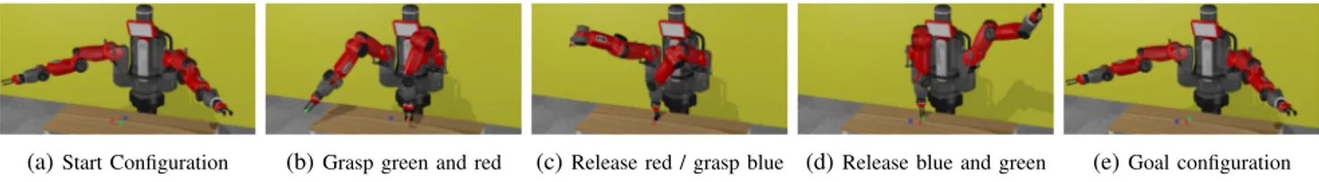
1) NAMO and Manipulation: Manipulation-RRT is im-plemented in the module hpp-manipulation. This al-gorithm can be used indifferently for complex manipulation and NAMO. A first example scenario shows the Baxter robot permuting the positions of three boxes on a table (Fig. 4). The only inputs specified are the start and goal configurations of the boxes, as well as the constraint graph from Fig. 3, extended to handle a third box. In the second example the Romeo robot puts an object in a fridge (Fig. 5 while maintaining equilibrium. Again, only the final position of the object is specified. With the constraint graph the door is automatically grasped and openend. These two examples are developed in [20].

2) Gradient-based path optimization: hpp-core pro-vides a gradient-based path optimizer to refine the indirect paths generated by probabilistic planners [22]. The algorithm is a Linearly Constrained Quadratic Program that modifies the waypoints of a path to make it shorter. To do so, constraints are automatically generated between the objects that might collide during the optimization. Thus, only part of the configuration variables are constrained at some points of the path, while others are optimized. A result based on a PR2 robot avoiding a table is presented in Fig. 6.

3) Acyclic contact planning: is a class of problem where an under-actuated multiped robot must be in contact at every configuration to maintain static equilibrium, and exert the forces allowing it to move. We address this issue sequen-tially: first, a path is computed for the root of the robot, in a low dimensional space. Then along this path, a discrete sequence of “key” contact configurations is computed. These key frames are interpolated dynamically using a 3D pattern-generator [23]. The first two steps are implemented in HPP, using a planner called RB-RRT [24], [25], for Reachability-Based planner. RB-RRT uses extensively position and orien-tation constraints to maintain and generate contacts. It also takes advantage of the flexibility of HPP to easily replace the default sampling method for a variant of OB-PRM [26]. The pattern generator is implemented thanks to the Pinocchio dynamics library [27], soon to be integrated with HPP. A stair climbing using a handrail scenario is illustrated in Fig. 7.

4) Elastic rod planning: A special case of manipulation planning for an extensible elastic rod, either collision-free

(a)Start Configuration (b)Grasp green and red (c)Release red / grasp blue (d)Release blue and green (e)Goal configuration Fig. 4: A complex manipulation example for the Baxter robot. The task is to swap the position of three boxes. This requires a sequential task decomposition, automatically inferred by Manipulation-RRT .

(a)Start Configuration (b)Grasp object (c)Open fridge / place object (d)Close fridge door (e)Goal configuration Fig. 5: A complex manipulation example for the Romeo robot. The task is to put an object in a fridge. The planner automatically infers that the fridge door must be opened.

Start configuration Goal configuration

Fig. 6: Illustration of the path optimization algorithm. Given the start and goal configurations shown on the left, a rough path is computed with a sampling-based planner (top). The path is reduced to limit the motion of all joints (bottom). The red (resp. blue) curve denote the path followed by the right effector along the motion.

Start configuration wut wut wut Goal configuration

Fig. 7: Multi-contact planning for the HRP-2 robot climbing stairs using a handrail, a typical scenario proposed by the DARPA challenge. Through a connection with the Pinocchio library, the plan can be executed on the real robot (right).

or in contact [28]. We assume the rod can be handled by grippers at one or both extremities. External libraries (QSERL and XDE) are used to compute the deformation and the dynamics of the rod. This demonstrates the compatibility of HPP with external software. A dedicated steering method, which uses these libraries, is implemented within a slightly modified RRT algorithm. This implementation allows to plan a motion for an elastic rod egressing from a complex engine through a small hole (Fig. 8).

VI. CONCLUSION

This paper introduces HPP, the Humanoid Path Planner, a constraint-based motion planning software. HPP provides

a framework for easily testing and implementing algorithms inspired from recent contributions from the scientific com-munity, including Navigation and Among Movable Obsta-cles, manipulation and acyclic contact planning.

To our knowledge no existing software provides imple-mentations to address these issues in a unified manner. While in theory it is possible to extend existing softwares to implement these algorithms, integrating constraint-related features from the conception of HPP allows for a simple architecture, providing many helper methods to facilitate the use of complex notions such as differentiable functions and constraint graphs. Moreover, this unified architecture also comes with excellent performances, and HPP is able to

Start configuration wut wut wut Goal configuration Fig. 8: Extraction of a deformable elastic rod from an engine. The green rod shows the goal configuration, the yellow shows the motion computed from the initial configuration(left picture). Engine model courtesy of Siemens-KineoCAM.

compete with the best actual planning implementations on the standard benchmarks.

Bindings of the API using a CORBA architecture allow for fast prototyping and testing in Python, and a simple integration with other softwares. It is also delivered with benchmarking tools compatible with the OMPL benchmark API, and Blender export functions for high-quality rendering. HPP is already a mature software, which has been used to implement several new scientific contributions, also demon-strated in the companion video. They demonstrate the ability to integrate HPP with complex third-party softwares, and offer a glimpse of the future features that HPP will be provided with. Among those, the integration of the Pinocchio dynamic library holds the promise of a seamless framework between motion planning and its execution on a real robot.

REFERENCES

[1] J. T. Schwartz and M. Sharir, “On the piano movers’ problem i. the case of a two-dimensional rigid polygonal body moving amidst polygonal barriers,” Communications on Pure and Applied Mathematics, vol. 36, no. 3, pp. 345–398, 1983. [Online]. Available: http://dx.doi.org/10.1002/cpa.3160360305

[2] L. E. Kavraki, P. Svestka, J.-C. Latombe, and M. H. Overmars, “Prob-abilistic roadmaps for path planning in high-dimensional configuration spaces,” IEEE Transactions on Robotics and Automation, vol. 12, no. 4, pp. 566–580, August 1996.

[3] S. M. LaValle, “Rapidly-Exploring Random Trees: A New Tool for Path Planning,” In, vol. 129, no. 98-11, pp. 98–11, 1998.

[4] T. Lozano-P´erez, “Spatial planning: A configuration space approach,” IEEE Trans. on Computers, vol. C-32, pp. 108–120, 1983. [Online]. Available: http://lis.csail.mit.edu/pubs/tlp/spatial-planning.pdf [5] I. A. S¸ucan, M. Moll, and L. E. Kavraki, “The Open Motion Planning

Library,” IEEE Robotics & Automation Magazine, vol. 19, no. 4, pp. 72–82, December 2012, http://ompl.kavrakilab.org.

[6] R. Diankov and J. J. Kuffner, “Openrave: A planning architecture for autonomous robotics,” Robotics Institute, Caneggie Mellon University, Pittsburgh, Pennsylvania, Tech. Rep., 2008.

[7] Wikipedia, “Kineo cam — wikipedia, the free encyclopedia,” 2015, [Online; accessed 19-February-2016]. [Online]. Available: https: //en.wikipedia.org/w/index.php?title=Kineo CAM&oldid=647097086 [8] T. Bretl, “Motion planning of multi-limbed robots subject to

equilibrium constraints: The free-climbing robot problem,” The Int. Journal of Robot. Research (IJRR), vol. 25, no. 4, pp. 317–342, Apr. 2006. [Online]. Available: http://cpc.cx/gAs

[9] M. Stilman and J. Kuffner, “Navigation among movable obstacles: Real-time reasoning in complex environments,” in Proceedings of the 2004 IEEE International Conference on Humanoid Robotics (Humanoids’04), vol. 1, December 2004, pp. 322 – 341.

[10] M. Levihn, L. Kaelbling, T. Lozano-Perez, and M. Stilman, “Fore-sight and reconsideration in hierarchical planning and execution,” in Intelligent Robots and Systems (IROS), 2013 IEEE/RSJ International Conference on, Nov 2013, pp. 224–231.

[11] T. Sim´eon, J.-P. Laumond, J. Cort´es, and A. Sahbani, “Manipulation Planning with Probabilistic Roadmaps,” The International Journal of Robotics Research (IJRR), vol. 23, no. 7-8, pp. 729–746, 2004.

[12] K. Harada, T. Tsuji, and J.-P. Laumond, “A manipulation motion plan-ner for dual-arm industrial manipulators,” in Robotics and Automation (ICRA), 2014 IEEE International Conference on. IEEE, 2014, pp. 928–934.

[13] F. Burget, A. Hornung, and M. Bennewitz, “Whole-body motion planning for manipulation of articulated objects,” in Robotics and Automation (ICRA), 2013 IEEE International Conference on, May 2013, pp. 1656–1662.

[14] S. Nakaoka, “Choreonoid: Extensible virtual robot environment built on an integrated gui framework,” in System Integration (SII), 2012 IEEE/SICE International Symposium on, Dec 2012, pp. 79–85. [15] M. Quigley, K. Conley, B. P. Gerkey, J. Faust, T. Foote, J. Leibs,

R. Wheeler, and A. Y. Ng, “Ros: an open-source robot operating system,” in ICRA Workshop on Open Source Software, 2009. [16] R. M. Murray, S. S. Sastry, and L. Zexiang, A Mathematical

Introduc-tion to Robotic ManipulaIntroduc-tion, 1st ed. Boca Raton, FL, USA: CRC Press, Inc., 1994.

[17] J. Pan, S. Chitta, and D. Manocha, “Fcl: A general purpose library for collision and proximity queries,” in Robotics and Automation (ICRA), 2012 IEEE International Conference on. IEEE, 2012, pp. 3859–3866. [18] S. Dalibard, A. El Khoury, F. Lamiraux, A. Nakhaei, M. Ta¨ıx, and J.-P. Laumond, “Dynamic walking and whole-body motion planning for humanoid robots: an integrated approach,” The International Journal of Robotics Research, vol. 32, no. 9-10, pp. 1089–1103, 2013. [19] M. Stilman, “Global manipulation planning in robot joint space with

task constraints,” 2010.

[20] J. Mirabel and F. Lamiraux, “Constraint graphs: Unifying task and motion planning for navigation and manipulation among movable obstacles,” 2016. [Online]. Available: http://cpc.cx/eOE

[21] Blender Online Community, Blender - a 3D modelling and rendering package, Blender Foundation, Blender Institute, Amsterdam. [Online]. Available: http://www.blender.org

[22] M. Campana, F. Lamiraux, and J. P. Laumond, “A gradient-based path optimization method for motion planning,” 2016. [Online]. Available: http://cpc.cx/gAr

[23] J. Carpentier, S. Tonneau, M. Naveau, O. Stasse, and N. Mansard, “A versatile and efficient pattern generator for generalized legged locomotion,” in To appear in Proc. of IEEE Int. Conf. on Robot. and Auto (ICRA), Stockholm, Sweden, May 2016.

[24] S. Tonneau, N. Mansard, C. Park, D. Manocha, F. Multon, and J. Pettr´e, “A reachability-based planner for sequences of acyclic contacts in cluttered environments,” in Int. Symp. Robotics Research (ISRR), (Sestri Levante, Italy), September 2015, 2015.

[25] S. Tonneau, A. D. Prete, J. Pettr´e, C. Park, D. Manocha, and N. Mansard, “An efficient acyclic contact planner for multiped robots,” technical report, 2016. [Online]. Available: https://hal.archives-ouvertes.fr/hal-01267345v2/document

[26] N. M. Amato, O. B. Bayazit, L. K. Dale, C. Jones, and D. Vallejo, “Choosing good distance metrics and local planners for probabilistic roadmap methods,” IEEE T. Robotics and Automation, vol. 16, no. 4, pp. 442–447, 2000.

[27] N. Mansard, F. Valenza, and J. Carpentier, “Pinocchio: Fast forward inverse dynamic for multibody systems,” 2014. [Online]. Available: http://stack-of-tasks.github.io/pinocchio/index.html

[28] O. Roussel, A. Borum, M. Ta¨ıx, and T. Bretl, “Manipulation planning with contacts for an extensible elastic rod by sampling on the submanifold of static equilibrium configurations,” IEEE International Conference on Robotics and Automation (ICRA 2015), May 2015. [Online]. Available: https://hal.archives-ouvertes.fr/hal-01096543