Collaborative UAV path planning with deceptive strategies

Collaborative UAV Path Planning with Deceptive

Strategies

by

Philip J. Root

Submitted to the Department of Aeronautics and Astronautics

in partial fulfillment of the requirements for the degree of

Masters of Science in Aeronautical Engineering

at the

MASSACHUSETTS INSTITUTE OF TECHNOLOGY

May 2005

@

Massachusetts Institute of Technology 2005. All rights

Author...

. . .. . . . . .. . . . . . . . . .

Department of Aeronautics and Astronautics

February 18, 2004

Certified by...

Eric Feron

Associate Professor of Aeronautics and Astronautics

Thesis Supervisor

P A

A

I

Accepted by ...

...

.

...

Jaime Peraire

Professor of Aeronauties and Astronautics

Chair, Committee on Graduate Students

AERO

)MA

4 _{SETTS INSTITUTE}

OF TECHNOLOGY

JUN 2 3 2005

Collaborative UAV Path Planning with Deceptive Strategies

by

Philip J. Root

Submitted to the Department of Aeronautics and Astronautics on February 18, 2004, in partial fulfillment of the

requirements for the degree of

Masters of Science in Aeronautical Engineering

Abstract

In this thesis, we propose a strategy for a team of Unmanned Aerial Vehicles (UAVs) to perform reconnaissance of an intended route while operating within aural and visual detection range of threat forces. The advent of Small UAVSs (SUAVs) has funda-mentally changed the interaction between the observer and the observed. SUAVs

fly at much lower altitudes than their predecessors, and the threat can detect the

reconnaissance and react to it. This dynamic between the reconnaissance vehicles and the threat observers requires that we view this scenario within a game theoretic framework. We begin by proposing two discrete optimization techniques, a recur-sive algorithm and a Mixed Integer Linear Programming (MILP) model, that seek a unique optimal trajectory for a team of SUAVs or agents for a given environment. We then develop a set of heuristics governing the agents' optimal strategy or policy within the formalized game, and we use these heuristics to produce a randomized algorithm that outputs a set of waypoints for each vehicle. Finally, we apply this final algorithm to a team of autonomous rotorcraft to demonstrate that our approach operates flawlessly in real-time environments.

Thesis Supervisor: Eric Feron

Acknowledgments

First, I would like to thank my parents who infused me with a sense of undying curiosity at a young age. May they never stop peering in creation's corners for truth, trivia, and teaching subjects.

To my advisor, Eric Feron, thank you for your support, guidance, and feedback through this endeavor. My enjoyable experience at the Institute was entirely due to the esprit de corps you foster within your group. May your accent be ever baffling, your handwriting ever cryptic, and your brilliance and flair ever inspiring.

To my second advisor, Andy Mawn, you opened opportunities for me throughout the Army, and this research reflects your pragmatism and purpose. We as a nation are fortunate to have professionals passionate in their support of the Armed Forces such as you. Illegitimus Non Carborundum.

To my de facto mentor, Jan De Mot, I sincerely appreciate your investment in time and patience in this research. So much of this document is inspired by your genius. May your thesis preparations go quickly, but may your newlywed bliss last forever.

To my brother in Perl, Rodin Lyasoff, your comedy, coffee, and computing skills kept this dream afloat. It is an honor for me to have a son who will enjoy your avuncular influence for years to come. May you continue to propagate in others the belief that limits are entirely a mental construct.

To our dear friends, Mario and Tricia Valenti, thank you for your hospitality. May your son bring you more happiness than you can imagine.

To my lab mates, Masha Ishutkina, Farmey Joseph, Greg Mark, Tom Schouwe-naars, Mardavij Roozbehani, Olivier Toupet, Jerome Le Ny, and others, thank you for your camaraderie. You continue to make this a great lab to work and play. May your journeys be as satisfying as mine was with you.

To my wife and friend, Kristin, your enduring patience, motivation, and honesty have inspired me to greater accomplishments. Every moment in your presence is an adventure, and I pray that you enjoy this journey as much as I do.

Finally, to my Lord and Savior, Jesus Christ, who continues to shower me with blessings (e.g. the individuals listed above.) May my actions reflect my love for You.

Contents

1 Introduction 17 1.1 Threat Model . . . . 18 2 Exact Methods 21 2.1 Relevant Work . . . . 21 2.2 _{Problem Formulation . . . . 22} 2.3 _{Iterative Methods . . . . 29} 2.4 Linear Programming . . . . 39 3 Mixed Strategies ₄₉ 3.1 Relevant Work . . . . 49 3.2 Problem Formulation . . . . 50 3.3 Problem Solution . . . . 60 3.3.1 Solution Outline . . . . 60 3.3.2 Path Generation . . . . 62 3.3.3 Path Evaluation . . . . 63 3.4 _{Example Application . . . . 65} 4 Experimental Results ₇₁ 4.1 Statistical Analysis . . . . 71 4.2 Flight Testing . . . . 76

5 Conclusions and Future Work 83 5.1 Thesis Summary . . . . 83

List of Figures

2-1 Simplified environment with intersection of large and small road. . 22

2-2 Set of edges E1 . . . . 22

2-3 Set of nodes V . . . . 22

2-4 Set of edges E2 required to connect every node in V to every other 22 2-5 Environment used in game development . . . . 26

2-6 Tmax=2... ... ... 26

2-7 T ax 4 . . . . 27

2-8 T max _{= 3 . . . . 27}

2-9 The state s = (d, XA, XB, tA, tB) used in the iterative methods. .... 30

2-10 Example of band propagation through simple graph. . . . . 32

2-11 Graph G = (V, E) superimposed over Charles river environs. . . . . . 34

2-12 Optimal trajectory of two agents using recursive value iteration. . . . 35

2-13 Example of suboptimal trajectory using min

Z

max cost function. . . 36

2-14 Notional trajectory using min max

E

cost function. . . . . 37

2-15 Notional trajectory using min

E

max cost function. . . . . 38

2-16 Notional trajectory using min

E

max cost function in the limit as |a rl

>>

|ladl. . . . .

38

2-17 Optimal trajectory of two agents using linear programming algorithms. 43 2-18 Sequence of Exact Methods Solutions . . . . 45

2-19 Optimal trajectory of two agents using linear programming with three cycles highlighted . . . . 46

3-2 Game One: Tmax = 2 leads to mixed strategies. . . . . 54

3-3 Game Two: Tmax = 4 leads to mixed strategies. . . . . 54

3-4 Game Three: Tmax = 3 leads to mixed strategies. . . . . 54

3-5 Game Four: Tmax = 3 leads to mixed strategies. . . . . 56

3-6 Game Five: Tmax = 3 with non-sequential coverage leads to mixed strategies. . . . . 57

3-7 Simplified environment with intersection of large and small road. . . . 66

3-8 Set of edges E1 . . . . 66

3-9 Set of nodes V . . . . 66

3-10 Set of edges E2 required to connect every node in V to every other . 66 3-11 Graph structure and notation. Vertices are circles, deception routes are light lines, the reference trajectory is the dark line and areas of interest are squares. . . . . 67

3-12 (a) Complete trajectory for two agents. (b) Trajectory from origin to 30 minutes. (c) Trajectory from 30 minutes to 60 minutes. (d) Trajectory from 60 minutes to completion. . . . . 68

3-13 (a) Complete observations from agents' trajectories. (b) Observations from origin to 30 minutes. (c) Observations from 30 minutes to 60 minutes. (d) Observations from 60 minutes to completion . . . . 69

4-1 Autonomous model helicopter used for all flight tests. . . . . 77

4-2 Environment used to demonstrate algorithm. . . . . 78

4-3 Set of trajectories output from algorithm . . . . 79

4-4 Trajectory of Vehicle One. . . . . 80

4-5 Trajectory of Vehicle Two. . . . . 81

List of Tables

4.1 Factors and their experimental ranges . . . . 72 4.2 Correlation between factors and data for all iterations . . . . 73 4.3 Correlation between factors and data only for iterations that converged 74 4.4 Correlation between factors and data only for iterations that converged

given Tmax = 2500 sec . . . . 74 4.5 Correlation between factors and data only for iterations that converged

given Tmax = 3000 sec . . . . 75 4.6 Correlation between factors and data only for iterations that converged

given Tmax = 3500 sec . . . . 75 4.7 Correlation between factors and data only for iterations that converged

List of Algorithms

2.1 Recursive value function calculation for wave propagation . . . . 31 2.2 Recursive value function calculation for band propagation . . . . 33 3.1 Path generation algorithm . . . . 64

List of LP Models

2.1 Shortest Path Problem Model . . . . 40

2.2 Deceptive Trajectory Planning Model . . . . 47

Chapter 1

Introduction

Unmanned Aerial Vehicles (UAVs) have become increasingly ubiquitous in the past decade as technology pertaining to autonomy, rugged aircraft design, and commu-nications continues to mature. While not confined to military roles, their utility in combat scenarios has fueled their spreading influence. Beginning originally as large unmanned aircraft, UAVs have continued to shrink in size to support smaller mil-itary units. Once confined to support operations on a strategic and national level, the first Persian Gulf war saw their use at the Division level[25]. In the following decade and as UAV technology continued to improve, UAV use migrated down to the Battalion and Company level in time for the second Persian Gulf war[21]. The impact of this change is profound in several ways. First, the vehicles, avionics, and optics are necessarily smaller to support this unique role. Lower level military units displace more often, and therefore do not have a fixed base from which to operate. They have limited maintenance support as they deploy. Second, these vehicles re-quire an increasing workload for the operators as their capabilities improve. A typical

UAV system requires one operator and one mission controller

/

intelligence analyst for any reconnaissance. This represents an increase in responsibilities for the mili-tary unit as these operators must be organic to the unit and are not often attached. Third and most importantly for this thesis, the UAVs come in closer contact to the enemy. These vehicles fly at much lower altitudes than their larger brethren, and they frequently come within visual and aural detection ranges of the enemy[3]. This

fundamentally changes the underlying assumptions when developing reconnaissance missions for these aircraft. Threat forces can now react to UAV reconnaissance be-cause they can detect these aircraft without radar but rather just by sight and sound; UAVs are no longer relegated to high altitudes outside of human detection range, but it is insufficient to maintain the same doctrine at these lower flight regimes. Addi-tionally we must consider the potential of operating SUAVs in teams to counter the reactions of a dynamic threat to UAV detection.

In this thesis we will explore several different methods of determining "optimal" flight paths for a team of UAVs operating within detection range of a threat. We begin with two similar exact methods to perform discrete optimization of the given problem and highlight the shortcomings of these approaches. The interaction between reconnoitering UAVs and the enemy forces is dynamic by nature, so we simplify our model of these interactions into a game theory framework and argue several heuristics that emerge. We use these heuristics to create an ad hoc algorithm relying heavily on mixed strategies and randomness to develop feasible and deceptive path sets for this team of UAVs. Finally we apply this algorithm to a team of two autonomous rotorcraft to test the utility of our approach to real time applications. First we must introduce our model of the enemy forces.

1.1

Threat Model

The future of combat will be marked by increasingly non-contiguous warfare where no clear delineation between opposing forces exists [16]. While history abounds with examples of such nonlinear combat operations such as the U.S. experience in Viet-nam, the Balkans, and Somalia, the Russo-Chechen conflicts exemplify this trend toward unconventional operations and in particular for operations in urban environ-ments [23]. We will adopt our model of the opposing forces largely from observations of these historical conflicts. To this end, we will refer to the belligerents as defenders and invaders as we introduce the problem, and more simply, as observers and agents as we formulate the problem and present a solution.In all of the above historical

exam-ples, defenders used a markedly similar command architecture emphasizing tactical dispersion. The defenders array themselves in a dispersed arrangement that does not offer the invaders a centralized target to attack. They rarely outwardly appear as com-batants and hence are indistinguishable from the local population. Spread uniformly throughout the city, these observers seek to capture as much intelligence as possible pertaining to the invader's intentions and actions. The defenders operate in largely independent cells while reporting sensitive information to a centralized headquarters via redundant means of communication such as cellular phones, landline phones, the Internet, and citizen band (CB) radios [18]. This headquarters collects these intel-ligence reports to identify any trends in the observations; any trends or correlations within the reports may identify the invader's future movements. If they deem the intelligence sufficiently credible, the defenders will establish a threat or ambush at the location of maximum likelihood of contact. This requires a timely shift from passive observation to active defense, and the headquarters must operate as rapidly as pos-sible. In a dense urban environment, this distributed arrangement with centralized planning offers the defenders a much more complete analysis of the current situation than often available to the invader. Additionally, the thorough observer dispersion makes it improbable that the invader can maneuver without being observed [20].

The invader possesses roughly the opposite advantages and attributes. Composed of a large number of soldiers, vehicles, and materiel, the invader enjoys numerical and weapons superiority. This structure, however, makes it impossible for the invader to operate without being observed. While the defenders are identical in appearance to the local population, their foreign uniforms and military vehicles easily identify the invaders. Isolated in more secure areas of the urban environment, the defender must routinely move through areas observed by the defender for offensive or logistical reasons. These convoy movements are highly susceptible to threats, and the invader takes every effort to ensure their security. Before deploying along an intended convoy route from an initial position to the objective, the invader identifies critical areas that can influence this movement. While some of these areas may be likely ambush sites along the intended convoy route, others may be known or predicted defender locations.

Reconnaissance of these critical areas in addition to observing the intended convoy route allows the invader to ensure the security of the convoy as much as feasible[14, 15].

Collaborative UAV path planning is a well-established body of work in research communities, and many have sought to optimize the trajectories of a team of UAVs. We will delay introducing relevant research until sections 2.1 and 3.1 to motivate the

Chapter 2

Exact Methods

This chapter seeks to find an optimal routing for a team of collaborative UAVs given the military motivation presented in Section 1. Specifically we develop two similar objective functions and apply discrete optimization techniques to determine if there exists a unique optimal solution to the problem. All efforts pertaining to randomness are postponed to Chapter 3. We begin by introducing some relevant work done in path planning optimization in Section 2.1. Section 2.2 introduces notation and the problem formulation used throughout this chapter. We propose a recursive algorithm and a linear programming model to solve this problem in Sections 2.3 and 2.4, respectively. Both sections end with an application of their proposed solutions to an example environment.

2.1

Relevant Work

It is feasible to model the problem as a discrete optimization resulting in a unique op-timal solution that satisfies all mission requirements while minimizing

/

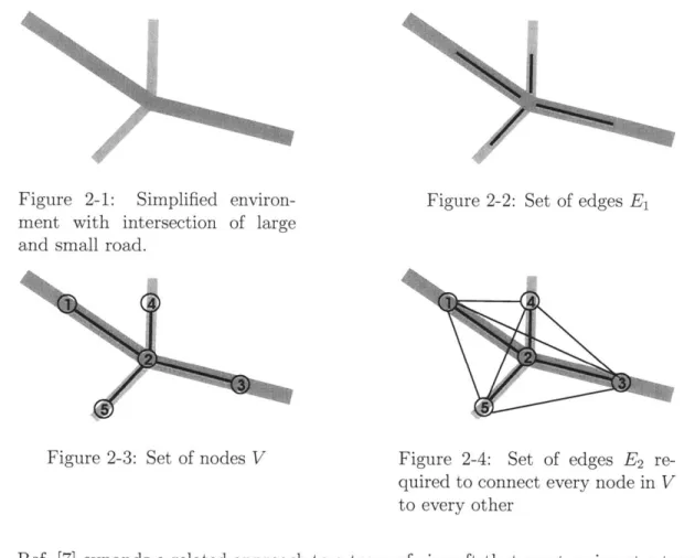
maximizing some cost function. Research pertaining to UAV path planning in adversarial envi-ronments abounds. Ref. [4] determines the shortest path through a Voronoi graph imposed over known enemy radar positions. This shortest path then serves as an initial condition for a second phase that creates a dynamically feasible aircraft trajec-tory using virtual masses and force field to develop smoothed trajectories. Similarly,

Figure 2-1: Simplified

environ-ment with intersection of large and small road.

Figure 2-3: Set of nodes V

Figure 2-2: Set of edges E1

Figure 2-4: Set of edges E2

re-quired to connect every node in V to every other

Ref. [7] expands a related approach to a team of aircraft that must arrive at a target at designated times. Each aircraft determines its optimal path in a two-step approach

markedly similar to [4], and a higher level coordination agents specifies the temporal

spacing commands necessary for all agents to arrive on target as required. Zabarankin et. al. [26] demonstrate the utility of combining analytic optimization techniques with network flow methods when minimizing the radar cross signature of an aircraft sub-ject to multiple threat radar locations. We begin by formulating the problem as a discrete optimization and then present two alternative solution techniques.

2.2

Problem Formulation

We desire to model the urban environment as a complete undirected graph for use in analysis and optimization. Figure 2-1 depicts a highly simplified environment containing the intersection of a large and small street. We begin by creating a set of

edges along all roads and streets. Thus we populate the set Ei of edges such that each edge is of similar length and the endpoints of each edge egy = (vi, vj) are spread uniformly (see Figure 2-2). The sets of nodes V = {vi}, i = 1 ... n are located along these roads and particularly at road intersections (see Figure 2-3). We complete the set of edges E is the union of E1 and E2 where E2 represents the set of edges necessary

to complete the graph. In particular, E2 contains all the edges eij ( E1 connecting

vertices vi E V with vj E V and hence do not correspond to a street in the urban environment (see Figure 2-4). Thus the graph G = (V, E) is complete in that there exists an edge egj = (vi, vi) for all i = 1 ... nv and

j

= 1... no, and it is undirected in that eij = eji.

We define a set Em C Ei of edges associated with the streets that satisfy certain constraints. For example, for a heavy vehicle to traverse a particular street, the road surface must have sufficient width, minimum turning radius, and load carrying capability. These qualities are highly desirable to support military convoys, and Em represents the set of streets feasible for heavy vehicle traffic. In Figure 2-4, Em consists of only those edges along the larger road e12 and e23. Edges e24 and e25 are in E1 but

do not satisfy the constraints necessary to belong in Em.

Additionally, given is a set of vertices VA E V that are associated with critical urban areas with probable threat presence. UAVs must reconnoiter these areas to detect threats and attempt to determine the threat course of action.

We define a path p of length n as a sequence of edges p = {eie, e2 ,..., e}, ei =

(vi, v2), e2 = (v2, v3), ... , en = (vn, vn+1) [13]. We denote a special path, the reference trajectory, that corresponds to the intended convoy route such that the path pr = {e[}, for i = 1,. .. , nr. Additionally, we denote the initial vertex v, and final vertex vt and choose the reference trajectory such that ei E E1 , for i = 1, . .. , nr. The main task

of the UAVs is to determine whether p, is threat-free by observation. In particular, every edge of pr is traversed and observed by at least one UAV.

Finally the fundamental limitation in UAV performance is endurance governed by fuel limits. We model this constraint as a limit on maximum mission time, Tma,. For each edge ej (E E we specify an associated time tij to traverse the edge. For

ei E El, ti represents the flight time required to follow the associated street. For

eij E E2, tij is the time required to travel the length of the straight line connecting vi

and v. Additionally, we expect the UAVs to loiter at each vertex vi E VA for time toj. While it is safe to assume that flight vehicles will operate at different configurations throughout the mission and hence have different fuel consumption rates during a loiter versus flying straight and level, we simplify the dynamics of the model by restricting our constraint to only consider time. Thus for each vehicle:

tpi ~ ij + vi 5 max

eij Epi vi EpI

Given this notation describing the environment, we can begin to create feasible sets of paths for our team of vehicles. The following problem formulation summarizes the constraints listed thus far, but does not include any measures of deception.

Problem 1 (Constrained Shortest Path Problem) Given the complete, undi-rected graph G = (V, E) and N agents. Let p, {e }, for i = 1,... ,n, represent the reference trajectory, and VA = {vi} C V represent the areas of interest. Let tij represent the time required to travel on edge eij and tv, represent the expected loiter time at node vi. Let pi {ei, eI,... , e'} represent the path of vehicle i.

A feasible set of trajectories P = {pi} for i = 1... N agents satisfies the following constraints.

1. Each edge in the reference trajectory must be traversed by at least one agent,

eij E P for all eij E pr.

2. Each area of interest is visited by at least one agent, vi C P for all vi E VA. 3. Each agents' path requires less then the maximum time allowed,

p = :ij E vi 5max

eigjpi t vi pi

Find the optimal set of feasible trajectories P* E P that minimizes the maximum

This problem can be viewed as a modified shortest path problem with several additional constraints. This formulation falls short of exactly modeling the problem at hand. Specifically, there is no mention of the role of the enemy and our attempts to remain unpredictable. While we do try to minimize the time required for each agent tpi, it is also important for each vehicle with excess capacity to maximize deception. Deception, however, is a difficult measure to quantify at this point, as it is usually a subjective evaluation by a human operator. Nevertheless, we pose the following heuristics as a means to begin to quantify the deceptive efforts of a given trajectory. It is possible for a convoy originating at v, and terminating at vt to take any combination of feasible edges e e Em. Any enemy cognizant of this will then seek

to determine any information that indicates that one edge is more likely than an-other. Specifically, the observation of UAVs reconnoitering over feasible edges tends to increase the probability that a convoy will traverse that edge imminently. It is therefore important for the team of UAVs to traverse as many feasible edges as possi-ble to increase the difficulty of identifying the exact reference trajectory. In the limit the team of UAVs can cover the entire set of military-capable roads Em such that the enemy has no information as to the reference trajectory and must choose one route from within a uniform probability distribution.

We introduce a simple game at this point to clarify the feasible policies for both players. We propose a highly simplified version of the environment described above where Em consists of four edges, Y1, Y2, z1, and z2, as illustrated in Figure 2-5. If the source v, is to the left and the objective vt is to the right, there are two feasible paths between the two: Y = {yi, Y2} and Z = {zi, z2}. We refer to the set of these two feasible paths as R = {Y, Z}. _{We simplify the aircraft dynamics such that Tma,}

refers to the maximum number of edges that the UAVs can traverse.

There are two players to the game: player one, the team of UAVs; and player two, the threat observers. The game begins when player one traverses a set of edges in E such that p

c

E. Player two then observes all edges in player one's path p and

attempts to determine the reference trajectory pr C R. Player two selects a route r C R to establish an ambush. If player two surmises correctly such that r = Pr,

Y

y

1

y

2

zi

_Z

2

z

Figure 2-5: Environment used in game development

C

=

1.

0

Y1 Y2

Cz= 0.0

zi

z2

Figure 2-6: Tmax = 2

then player two wins; otherwise player one wins. There are two versions of the game depending on whether player two has perfect or imperfect information concerning player one's actions. Player two may have perfect information such that he observes all edges in player one's path p. In the other case, player two has imperfect information and only observes edge e E p with probability q.

Figure 2-6 depicts the first scenario where Tmax equals 2. Note that player one is constrained to traverse at least all edges for some r E R. If player two has perfect information, then it is trivial to identify p, E R; in this example Y must be the reference trajectory. If player two does not have perfect information, then he observes all edges in Y with probability q2

. However if player two is aware of the limited resources available to player one, i.e. Tmax = 2, then any observations along path Y confirms it as the reference trajectory.

___ _ _ A- Y =

0.5

Yi2

Z

0.5

zi

Z

2 Figure 2-7: Tmax = 4

Cy -

1.0

Y12

___

Cz

= 0.0

zi z₂ Figure 2-8: Tmax = 3

available to traverse all edges in R. Even with perfect information, player two cannot

determine p, and must choose a route r

E

R with uniform probability distribution.

This is the best case for player one, and it highlights the advantage of increasing

Tmax.

Finally, Figure 2-8 provides an example scenario where player one has excess

capacity. With Tmax = 3, player one can traverse all edges in Y as well as z₂. Again

given perfect information concerning player one's path p, player two can determine the reference trajectory with certainty. However, and most importantly for this research, if player two has imperfect information, there exists a probability that the reference

trajectory is path Z. For example, there is probability (1 - q)q2 _{that player two}

does not observe edge yi and observes edge y2 and z2. In this case, player two must

choose r E R with uniform probability distribution. This final case highlights the importance of traversing all possible edges in Em subject to the excess capacity after satisfying the constraint to cover p,.

We define deception routes as Ed C Em and Ed = {e3

}

( p,. Given limited

resources, it is imperative that the optimal team policy traverse as many edges eij E

Ed to maximize this arguable measure of deception and reduce the probability that

The set of feasible trajectories P contains a number of edges that intersect at a set

of common nodes v such that v is the union of all agent paths p' for i = 1 ... N. For

example, if one vehicle traverses the first edge of the reference trajectory e' = (vi, v2)

and a second vehicle traverses the next edge er = (v2, v3), the vehicles potentially

collide at node v2. From the perspective of an enemy observer on the ground, these

nodes where the path intersect draw increased attention. Continuing the previous

example, if the enemy observed two vehicles at node v2 at nearly the same time it

would be reasonable to conclude that node v2 is along the reference trajectory

We choose to alter the problem formulation to incorporate these measures of deception.

Problem 2 (Deceptive Shortest Path Problem) Given the complete, undirected

graph G = (V, E) and N agents. Let Pr = {e }, for i = 1, ... , nr represent the refer-ence trajectory, and VA = {vi} C V represent the areas of interest. Let tij represent the time required to travel on edge e j and tv represent the expected loiter time at node vi. Let pi = {ei, ei,... , e'} represent the path of vehicle i. Let v represent the set of common nodes from the set of all vehicle paths v = n pi for i = 1 ... N. Let a, > 1 be

a constant real cost factor for traveling on the reference trajectory such that the cost of traveling on any edge is cij = artij for all eij E Pr. Let ad < 0 be a constant real cost factor for traveling on a deception route such that the cost of traveling on any edge is cij = adtij for all eij E Ed. Otherwise cij = tij for all eij p, and eij 0 Ed.

A feasible set of trajectories P = {pi} for i = 1 ... N agents satisfies the following constraints.

1. Each edge in the reference trajectory must be traversed by at least one agent, ec G P* for all ej (E pr.

2. Each area of interest is visited by at least one agent, vi G P* for all vi

e

VA. 3. Each agents' path requires less then the maximum time allowed,

tpi=I:ti+(:t ;Tmax

4.

All vehicles maintain AT temporal spacing at common nodes v.

Find the optimal set of feasible trajectories P* E P that minimizes the maximum cost Cmax = maxi=1...N(cp) required for all agents where

ei p

D

2.3

Iterative Methods

We seek to solve Problem 2 using an iterative method inspired by lessons from

Dy-namic Programming (DP). DP is a modeling methodology that makes decisions in

stages. In its essence, it determines the optimal trade-off between current costs and costs incurred in the future based on the local decision or input. These costs are in terms of some objective function. A problem formulated using DP is often solved recursively where we find the optimal solution for all possible states at the last stage before progressing to the previous stage [1]. Our approach differs from pure DP in that our state must contain information on how we arrived at the current state; DP does not consider past information in determining optimal policies. While we ac-knowledge that our approach differs fundamentally from DP, we borrow a number of its precepts in constructing our algorithm. Thus we will present our iterative

algo-rithm that is inspired by DP while highlighting all deviations. We begin our analysis

constrained to the simple case of only two agents, A and B.

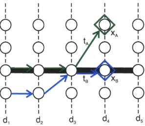
We begin by constructing the state vector s E S where S represents the entire state space. Specifically the state space has five elements S E R5: stage, di E D for i = 1, 2,... , nd, position, XA and XB, and time of the agents, tA and tB. Each stage

is a set of nodes, Vd C V such that V is the union of Vd for all stages in D. The position of each agent corresponds to a node within the graph XA E V and XB E V

and are constrained by the current stage such that if sd represents the feasibles states at stage d, then XA E sd and XB E Sd. Finally tA > 0 and tB 0 represent the time

I I |

XA

tA

I iiL XB

di

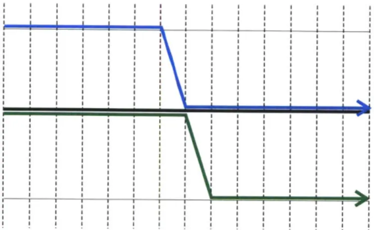
d2 d3 d4 d5

Figure 2-9: The state s = (d, XA, XB, tA, tB) used in the iterative methods.

that each agent arrives at its current position XA and XB. Figure 2-9 illustrates the

state s E S that we use in this iterative method on a simple graph. The dark black line represents the reference trajectory pr.

Our aim is to determine the optimal control at every state s E S. We define the

control space U and constrain the control actions available at each state u, E U for all s E S. These constraints originate from items (1) and (2) from Problem 2 such that

not all states are allowable. For example, if we constraint the agents to propogate linearly forward, then S is constrained to those states where at least one agent is

on the reference trajectory, XA E pr or XB E pr. Further, u, is constrained to those

control actions that maintain at least one agent on the reference trajectory. Similarly,

s and u, are constrained by the requirement to visit areas of interest. Finally, item

(4) of Problem 2 constrains s and hence u, to those cases where |tA - tB ;> AT.

Our goal is for each vehicle to share the cost of traveling on the reference trajectory and the benefit of traveling on the deception routes. Clearly it is feasible yet highly undesirable for one vehicle to traverse the entire reference trajectory while the second vehicle covers the deception routes. To prevent this strategy from being optimal we chose to minimize the maximum of the cost function for both agents. This form of a cost function yields nearly equal resultant costs in optimal solutions. This is reflected in the objective of Problem 2.

Given these definitions and constraints, we propose Algorithm 2.1 that seeks to find the optimal control at any state by recursively evaluating for each state feasible at a given stage. Again, this algorithm falls short of a strict implementation of DP

Algorithm 2.1 Recursive value function calculation for wave propagation J, = 0 for all s E Sdnd {Jnitialize cost function at the last stage}

J, = oc _{for all s ( Sdd}

{Iterate through all stages}

for d<-

di

fori=nd -1,...1 do

for xA G Sd do for XB E sd do

for tA E

s

8 _do for tB C Sd do

s <- (d, XAxBB, tA, tB) {Set

current state}

for u'

E

u, do

X' = U/

for u' E u, do

4B

=

U

s' <- (d

+

1, x' , ' , t' , t') {Set future state}

r(u'

u'B)=

max(c(xA,X) ₊ JIs, c(XB,X) + Js')

end for end for

(u*, u*) = arg minx,2x (r) {Find cost function minimum}

z* = U4

XB UB

(d±

+)

_{{Set optimal future state}}

J= max(c(xA, X*4) + J,., c(xB, X*8) + Js*) {Set optimal cost function

for current state}

end for end for end for end for end for

because the "time" state must contain information pertaining to the route taken to the

current state i.e. tA and tB. We found that these states although necessary to address

constraint (4) of Problem 2 greatly increased the computational complexity and time required for algorithm completion. Thus while Algorithm 2.1 is conceptually simple to comprehend, we proposed the following improvements to more closely address the problem statement.

I I i I I I I tB XBV tAX

di

d2 d d4 _d5

Figure 2-10: Example of band propagation through simple graph.

We chose to remove tA and tB in subsequent algorithms to reduce the state space

S and accelerate computation time. We also chose to harness these improvements to

allow for increasingly deceptive trajectories. Trajectories from Algorithm 2.1 behave as a linear wave of agents that cannot move backward or laterally between stages. This behavior is desirable to present the enemy observers with more random observations. We implemented this approach by creating bands of stages and thus increased the

number of allowable states s E sd. Figure 2-10 depicts the additional states s E Sd at

each stage. Constraints (1) and (2) are much more difficult to enforce with the larger control space u, E U but the algorithm remains largely the same. With the savings

from reducing the state s = R3 after eliminating tA and tB, we were able to store two

cost functions jA and jB at every state. It is trivial to impose constraint (4) after

trajectory optimization using a simple linear programming model to satisfy temporal spacing requirements while minimizing mission time. This approach is admittedly suboptimal but it represents a small sacrifice in optimality compared to the savings in computation time and complexity. While Algorithm 2.1 solves for the optimal trajectory considering temporal and spatial constraints, Algorithm 2.2 considers only spatial constraints. In the worst case we enforce the temporal spacing by deploying each agent AT apart; this may be acceptable for teams of a small number of agents,

but clearly this is undesirable as the number of agents increase. In general, if AT is very small compared to Tmax, then the costs of enforcing temporal spacing after executing Algorithm 2.2 for a team of limited size are acceptable.

Algorithm 2.2 Recursive value function calculation for band propagation

J, = 0 for all s E Sdnd _{{Initialize cost function at the last stage}}

J, = oc for all s 0 sdnd

{Iterate through all stages} for d<- di fori=nd-1,...1 do

for XA E sd do for XB E sd do

s <- (d, XA, XB) {Set current state} for U'A E u, do

X/4 = U/

for u' E u, do

B B

S' <- (d + 1, x' , ') {Set future state}

T(u, u'B) max(c(xA, X') + J , c(xB,

4)

+ j)

end for end for

(u*,us) = arg minxr,z x(T) {Find cost function minimum}

XB = UB

s* - (d

+

1, x* ,) {Set optimal future state}

J^ c(xA, x*) + J! {Set optimal cost function for current state}

JB c(xiB ) +JB

end for end for end for

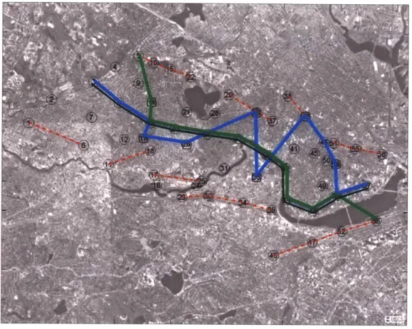
We implemented this algorithm using an environment modeled after the Charles river environs. Figure 2-11 depicts this environment; the reference trajectory is the solid line that extends from east to west; the deception routes are smaller dashed line fragments to the north and south of the reference trajectory. The areas of interest are squares while the nodes belonging to each stage are indicated by small dotted lines. We placed fifty-eight nodes in nineteen stages with five areas of interest and six deception routes. Populating an array of the node coordinates, we were able to determine the approximate length of each edge eij. We executed Algorithm 2.2 given the spatial constraints graphicly in Figure 2-11 Finally, Figure 2-12 illustrates the

Figure 2-11: Graph G = (V, E) superimposed over Charles river environs.

behavior of the algorithm on an this given urban environment where the two thick lines represent the trajectories of the team of two agents. These agents exhibit the desired behavior in that they swap positions on the reference trajectory twice during the mission. The large number of areas of interest in this environment preclude the agents from traversing any edges along deception routes. Instead we see that one agent traverses the majority of the reference trajectory while the second remains close to the reference trajectory and visits all areas of interest.

Algorithm 2.1 approaches a rigorous DP-like implementation, but a critical differ-ence exists in the calculation of the value function. The cost function of both

Algo-rithms 2.1 and 2.2 is to minimize the sum of the maximum costs: min(E max(cA, CB))

where c, represents the local cost for vehicle x. This is significantly different than the

common cost function minimize the maximum of the sum of the costs: min(max(E CA,

E

CB)).

We illustrate the significant implications of this subtle difference in Figure 2-13 where

Figure 2-12: Optimal trajectory of two agents using recursive value iteration.

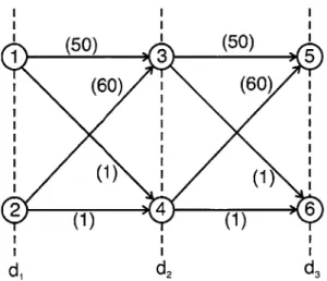
constraints of traversing the reference trajectory or areas of interest; we simply re-quire that the two agents are not located at the same node at the same stage. Thus for each stage di, d₂, and d3 there are only two states Sd; vehicle A is either on the top or bottom and vehicle B is the opposite. The algorithm begins by initializing the terminal cost at stage d3 to zero such that J, = 0 for all s E Sd. Recursively we move to stage d2 and begin by considering the state where vehicle A is at node 3, XA = 3. Here we find only two feasible control actions: UA = 5 and UB = 6; or

UA = 6 and UB = _{5. Our proposed cost function is min(E max(cA, CB)) and thus}

u* = 5 and u* = _{6 minimizes the maximum cost of 50 versus 60. Thus at state}

s' =A(d2, XA = 3, XB = 4), J, = 50 and J = 1 corresponding to the optimal control action. The solution is opposite and trivial if vehicle B is at the top at node 3. At stage di we must consider the local cost and the cost to go at the future state for all states s E Sd,. _{Regardless of the control action us, J,} = 50 for the vehicle at

(50)

(50)

1

3

5

(60)

(60)

d,

d2 d3

Figure 2-13: Example of suboptimal trajectory using min

E

max cost function.

the top node. Again we only have two possible states and we will only consider the case where vehicle A begins at node 1 such that XA = 1. Consider first UA = 3 and UB = 4; in this case CA = 50 + 50 and CB = 1 +1. The min(E max(CA, CB)) = 100-Consider now nA = 4 and UB = 3 where the resultant CA = 1

+50,

CB = 60

+50

and

min(E max(CA,

CB)) =110. Clearly u* u B =n 4 and J* = 100. Algorithm

2.1 returns paths PA = 13, es5} and pB = e24, e46} and J* = 100. A brief exhaustive search uncovers an improved set of trajectories p' = {e14, e45} and po = {e23, es6}

with J = 61.

This method of recursive value iteration has several benefits. Primarily, all of the value calculations can be done offline thus avoiding the need for realtime optimization. The optimal control is entirely determined by the state defined as the position of each agent at the current stage, and the cost function serves as a lookup table for optimal policies. Secondly, the cost function delivers the desired behavior. Namely, agent trajectories alternate between satisfying the constraints of the reference trajectory and the areas of interest, and the deception routes. We can alter the optimal trajectories by adjusting the weights assigned to the reference trajectory and deception routes se and unc to force the agents to swap positions on the reference trajectory more frequently.

Figure 2-14: Notional trajectory using min max

E

cost function.

not scale well. We constructed it in a parallel fashion to DP, and it suffers from the same "Curse of Dimensionality". Efforts to extend this algorithm to the case of three agents requires a polynomial increase in memory and computation time. Any attempts to extend the implementation beyond three vehicles were fruitless without further simplifying assumptions or changes in computational hardware. Increasing the number of stages or nodes within the graph also increases the complexity of the formulation to levels that are unsatisfactory for some environments.

The second most condemning observation about the algorithm is that we cannot accurately determine what the cost function represents. Mentioned above, the pro-posed cost function exhibits the desired behavior, but it is unclear what it represents exactly. The more traditional cost function choice min(max(E CA,

E

CB)) represents selecting the trajectory that minimizes the maximum total cost incurred by either vehicle. This does not suit our needs though in that the resulting set of trajectories do not swap locations on the reference trajectory often enough. Indeed, they only swap once in a general environment such that both agents accumulate the same total cost. Figure 2-14 illustrates the general behavior of two agents using a globally opti-mal trajectory from a min(max(E CA,

E

cB)) cost function. The reference trajectory is the dark line in the center of the figure and the deception routes are lighter lines at the top and bottom of the graph. Regardless of the weightings a, and ad, the trajectories do not change, and the behavior is stagnant.

. . . . . . . . . . . .

Figure 2-15: Notional trajectory using min max cost function.

Figure 2-16: Notional trajectory using min

Emax

cost function in the limit as jar

l>

|adl.

Conversely, the behavior of the algorithm changes drastically with respect to the relation between ar and ad with the proposed cost function min(E max(CA, CB). If

a, ~1_ -ad the set of trajectories behave in general as depicted in Figure 2-15 where the agents frequently swap between the reference trajectory and the deception routes. If

la,|l

>

ladl begin to form "triangles" along the reference trajectory. At each stage the algorithm seeks to minimize the maximum cost and hence the vehicles swap positions on the reference trajectory as often as possible. The benefit of traversing an edge on a deception route ad is offset by the requirement to swap on the reference trajectory more frequently and these typical "triangles" appear as Figure 2-16 depicts. Thus the min(E max(ca, CB)) cost function seeks to minimize the cost for the agent that

will incur the maximum cost from that state forward. The drawback of this approach is that ideally the algorithm should consider the cost incurred up to the current state to determine the optimal control. One solution would be to include the cost incurred as an element of the state, but the ramifications of this proposal would be intolerable. Namely to add information pertaining to the route taken to the current state would closely resemble an exhaustive search of all possible sets of trajectories

P. Worse yet, the computations required to determine the feasibility of every state

within the state space s C S would be astronomical. Thus the only way to improve the recursive algorithm would be to include the cost incurred in the state at which point the algorithm becomes an exhaustive search and computationally intractable.

2.4

Linear Programming

As discussed above, the recursive method has several distinct disadvantages: it re-quires a great deal of computation time; it does not scale well to additional vehicles or increased environment size; and the cost function poorly imitates the desired behav-ior. The algorithm can overcome these drawbacks only if it resorts to an exhaustive search of all feasible trajectories at which point the algorithm has no utility. Linear

programming (LP) offers solutions to a number of these limitations of the previous

approach. LP traditionally scales better than the recursive algorithmic approach, and the computation time required can be quite low if there is any underlying network structure to the problem. Thus emboldened, we begin to seek to implement LP to model and solve the proposed problem.

At first glance it would seem appropriate to apply a variant of the Shortest Path

Problem (SPP). The SPP seeks the route of minimum cost from source v, to target vt along edges within the graph G = (V, E). Indeed we can apply weights a, and

Cd to the applicable edges to more closely model the environment, but without

addi-tional constraints the solution is unsatisfactory; it avoids all edges along the reference

trajectory eg E Pr due to their high cost. This is unfortunate because LP solvers

Model 2.1 Shortest Path Problem Model

The following items constitute the model required for the LP solver. Parameters:

" Number of nodes n,

" Setof edges E={ei} forall i= 1... n, and

j=

1... n,

" Cost of edges cij " Source node vs " Target node vt " Number of agents N Variables:

o Flow on edge egj E E by vehicle k = 1... N: Xijk

Objective Function: Minimize the maximum cost of the path for the agents min max CijXi_jk

Constraints:

o Let

fi

_{represent the flow input at node vi such that}

_fi

_{= 1 for vi} =v,

fi

= -1 for vi = vt, and

f,

= 0 otherwise; then continuity requires

>

xijk+fi =Zxjik for i= 1...nv,

j =

1...nv, and k

=

1...

N

model.

Clearly the SPP Model falls well short of satisfying all the constraints outlined in Problem 2; specifically, it does not address the requirements to traverse all edges

egj E Pr and visit all nodes vi E VA. Before dismissing Model 2.1 we note one

fun-damental consequence of our future development. As stated, the Model is a network optimization problem, and if all the parameters are integer, then the resultant flow

Xijk is also integer. In essence we enjoy integrality for free in this formulation. In subsequent models we will pay dearly in computation time for demanding integral flow whereas it is a natural byproduct of this first simple formulation. Thus we must resort to Mixed Integer Linear Programming (MILP) to model our problem as we

can-not cast the problem as a variant of the continuous Shortest Path Problem. MILP incorporates integer variables into the model for use frequently as decision variables. While the addition of integer variables greatly increases the complexity of the model, it represents an extremely powerful method to model discrete problems.

As discussed above we must convert the decision variables to integer Xiik C Z to

ensure that the solution in nontrivial. Without this constraint the optimal solution

has fractional values for the decision variables Xjk along edges ei E pr. We will refer

to the decision variables as "flows" to indicate the underlying network optimization

structure to the problem. Hence we enforce integral flow Xiik along edges eij for

vehicle k =

1...

N.

We begin by modeling the requirement to traverse the reference trajectory. Since we force the flow along each edge to be integral and the flow along each edge on the reference trajectory eij E Pr to be positive, we can model the constraint as the sum of flows along the reference trajectory must exceed the number of edges along the reference trajectory.

Xijk > nr for all eij c Pr and k = 1... N

Similarly we can force the flow to visit every area of interest vi C VA. Again using the modeling power of integer decision variables we force the flow outgoing from node vi to be nonzero[2].

S

Xik for all vi E VA, eijcE and k= ... N

Previously we assigned constant tij to represent the time required to traverse edge

eij. We must constrain the solution such that each agent does not exceed the fuel

limitations specified by Tmax. Hence we state that total time for each agent must be less than or equal to Tmax.

Finally we are given a complete graph G = (V, E) where for every node vi and vj

there exists an edge eij that connects the two. Thus it is feasible for an agent to travel from one extreme of the graph to the other on one edge. This is arguably undesirable from the perspective of deceiving the enemy; we intend to display a nondeterministic pattern and traversing large distances in straight lines is anathema to our goal. Hence we offer a condition built upon the above argument to limit the length of the edges

adjacent to a given node. Two nodes vi and v are adjacent if there exists an edge eij

that connects them. Therefore we no longer consider the graph G = (V, E) complete

but rather create an adjacency matrix A where Aij = _{1 if there exists an edge eij}

connecting nodes vi and v. Specifically we choose to make two nodes adjacent if the

distance between them is less than rmax. Let vi - o| represent the distance between

nodes vi and v.

Aij =

1 forall vi EV and v 6EV if

||vi-vj||

<rin

0 otherwise

We incorporate the changes above into Model 2.2.

We intend to demonstrate Model 2.2 on the same Charles river environment de-picted in Figure 2-11. Specifically, we maintain the same coordinates for the fifty-eight nodes depicted as circles and the same reference trajectory depicted by the thin solid line. The deception routes are dotted lines, and the areas of interest are squares. The paths of the two agents in this scenario are the two thick solid lines. After parsing the output, Figure 2-17 illustrates the optimal vehicle trajectories P* determined by the LP model. We can make several observations regarding these trajectories. Funda-mentally we can verify that all spatial constraints are satisfied using the LP algorithm. Further we see that the trajectories are very similar between the recursive algorithm depicted in Figure 2-12 and the LP algorithm depicted in Figure 2-17. This supports our claim that these two algorithms are similar and based on the same underlying cost functions. Both algorithms inspire the desired behavior in the agents in that the alternate responsibilities on the reference trajectory with time on the deception routes. Perhaps the most striking feature of Figure 2-17 is the existence of trivial

Figure 2-17: Optimal trajectory of two agents using linear programming algorithms.

edges within the vehicles' paths pl. This is discussed at greater length later in this section.

Of course Model 2.2 does not address the requirement in Problem 2, item (4) to maintain a minimum temporal spacing of AT between vehicles at all points. It is nontrivial to include this constraint into the LP model because the decision variables

Xijk are not concerned with their relative sequence. Regardless of the discrete op-timization technique employed (i.e. Gomory cutting planes, Lagrangian relaxation, etc. [2]), we never consider the order in which we traverse the edges. Indeed the solution output from the LP solver contains only the integer values of X*3k, and we must reconstruct the optimal path from v to vt using the continuity condition. To incorporate the AT condition into the model would require an additional integer de-cision variable to determine the optimal sequencing of edges within the trajectory such that we can then impose the temporal spacing requirement. We are limited in this approach, however, in establishing AT to those common nodes v E P where the