Early Nested Word Automata for XPath Query Answering on XML Streams

HAL Id: hal-00966625

https://hal.inria.fr/hal-00966625

Submitted on 20 Feb 2015

HAL is a multi-disciplinary open access

archive for the deposit and dissemination of

sci-entific research documents, whether they are

pub-lished or not. The documents may come from

teaching and research institutions in France or

L’archive ouverte pluridisciplinaire HAL, est

destinée au dépôt et à la diffusion de documents

scientifiques de niveau recherche, publiés ou non,

émanant des établissements d’enseignement et de

recherche français ou étrangers, des laboratoires

Early Nested Word Automata for XPath Query

Answering on XML Streams

Denis Debarbieux, Olivier Gauwin, Joachim Niehren, Tom Sebastian,

Mohamed Zergaoui

To cite this version:

Denis Debarbieux, Olivier Gauwin, Joachim Niehren, Tom Sebastian, Mohamed Zergaoui. Early

Nested Word Automata for XPath Query Answering on XML Streams. Theoretical Computer Science,

Elsevier, 2015, pp.100-125. �10.1016/j.tcs.2015.01.017�. �hal-00966625�

Early Nested Word Automata for

XPath Query Answering on XML Streams

Denis Debarbieuxa,c_{, Olivier Gauwin}d,e_{, Joachim Niehren}a,c_{, Tom} Sebastianb,c_{, Mohamed Zergaoui}b

a_{Inria Lille,}b_Innovimax,c_LIFL,d_LaBRI,e_{University of Bordeaux}

Abstract

Algorithms for answering XPath queries on Xml streams have been studied intensively in the last decade. Nevertheless, there still exists no solution with high efficiency and large coverage. In this paper, we introduce early nested word automata in order to approximate earliest query answering algorithms for nested word automata. Our early query answering algorithm is based on stack-and-state sharing for running early nested word automata on all answer candidates with on-the-fly determinization. We prove tight upper complexity bounds on time and space consumption. We have implemented our algorithm in the QuiXPath system and show that it outperforms all previous tools in coverage on the XPathMark benchmark, while obtaining very high time and space efficiency and scaling to huge Xml streams. Furthermore, it turns out that our early query answering algorithm is earliest in practice on most queries

from the XPathMark benchmark.1

Keywords: Automata, logic, trees, nested words, streams, databases, document processing, Xml, XPath, Xslt, XQuery.

1. Introduction

Xmlis a major format for information exchange besides Json, also for Rdf linked open data and relational data. Therefore, complex event processing for Xml streams has been studied for more than a decade [14, 7, 26, 29, 5, 24, 15, 10, 25]. Query answering for XPath is a basic algorithmic task on Xml streams, since XPath is a language hosted by the W3C standards Xslt and XQuery.

Memory efficiency is essential for processing Xml documents of several gi-gabytes that do not fit in main memory, while high time efficiency is even more critical in practice. Nevertheless, so far there exists no solution for XPath query answering on Xml streams with high coverage and high efficiency. The

1

best coverage on the usual XPathMark benchmark [8] is reached by Olteanu’s Spex [26] with 22% of the use cases. The time efficiency of Spex, however, is only average, for instance compared to Gcx [29] which often runs in time close to the parsing time. We hope that this unsatisfactory situation can be resolved in the near future by pushing existing automata techniques forwards [14, 24, 10, 25].

In contrast to sliding window techniques for monitoring continuous streams [3, 19], the usual idea of answering queries on Xml streams is to buffer only alive candidates for query answers. These are stream elements which may be selected in some continuation of the stream and rejected in others. All space-optimal algorithms have to remove non-alive elements from the buffer, by outputting them or by discarding them. Unfortunately, this kind of earliest query answering is not feasible in polynomial time for XPath queries [6], as first shown by adapting counter examples from online verification [16]. A second argument is that deciding aliveness is more difficult than deciding XPath satisfiability [10], which is coNP-hard even for small fragments of XPath [4]. The situation is different for queries defined by deterministic nested word automata (Nwas) [1, 2], for which earliest query answering is feasible with polynomial resources [24, 11]. Many practical XPath queries (without aggregation, joins, and negation) can be compiled into small Nwas [10], while relying on non-determinism for modeling descendant and following axes. This, however, does not lead to an efficient streaming algorithm. The problem is that a cubic time precomputation in the size of the deterministic Nwa is needed for earliest query answering [11], and that the determinization of Nwas raises huge blow-ups in average (in contrast to finite automata).

Most existing algorithms for streaming XPath evaluation approximate earli-est query answering, most prominently: Spex’s algorithm on the basis of trans-ducer networks [26], Saxon’s streaming Xslt engine [15], and Gcx [29] which implements a fragment of XQuery. The recent XSeq tool [25], in contrast, restricts XPath queries by ruling out complex filters all over. In this way, node selection can always be decided with 0-delay [12] once having read the attributes of the node (which follow its opening event). Such queries are called begin-tag determined [5] if not relying on attributes. In this paper, we propose a new algorithm approximating earliest query answering for XPath queries that is based on Nwas. One objective is to improve on previous approximations, in order to support earliest rejection for XPath queries with negation, such as for instance:

//book[not(pub/text()=’Springer’)][contains(text(),’Lille’)] When applied to an Xml document for an electronic library, as below, all books published from Springer can be rejected once its publisher was read:

<lib>...<book>...<pub> Springer </pub>

...<content>...Lille...</content>...</book>...</lib> Spex, however, will check for all books from Springer whether they contain the

string Lille and detect rejection only when the closing tag </book> is met. This requires unnecessary buffering space.

As a first contribution, we provide an approximation of the earliest query answering algorithm for queries defined by Nwa [11, 24], while removing the assumption of determinism imposed there. The main idea to gain efficiency is that selection and rejection should depend only on the current state of an Nwa but not on its current stack. Therefore, we propose early nested word automata (eNwas) that are Nwas with two kinds of distinguished states: rejection states and selection states. Selection states are final and must always remain final, so that a nested word can be accepted, once one of its prefixes reaches a selection state. Symmetrically, rejection states can never reach a final state, so that a nested word can be rejected, once all non-blocking runs on a prefix reach a rejection state. We then present a new streaming algorithm for answering eNwa queries in an early manner. The basic idea is to run the eNwa for all possible candidates while determinizing on-the-fly, so that one can see easily whether all non-blocking runs of the nondeterministic automaton reach a rejection state, or whether one of them is selecting. The second idea is to share the stacks and states of runs of buffered candidates in the same state, so that the running time does not depend on the number of buffered candidates, but only on the number of states of the deterministic automaton discovered during the on-the-fly determinization. Our streaming algorithm with stack-and-state sharing for answering eNwas queries is original and nontrivial. It enables tight upper bounds for time and space complexity that we prove (Theorem 13).

As a second contribution, we show how to compile XPath expressions to small eNwa descriptors defining the same query. These descriptors allow to represent eNwas with large finite alphabets in a succinct manner, by replac-ing labels in eNwa rules by label descriptors. The label descriptor ¬a, for instance, stands for the set of all finitely many labels different from a. The target of our XPath-compiler are thus eNwa descriptors. For instance, the eNwadescriptors that our XPath compiler obtains for the XPath expressions Pn = child::a1/child::a2/.../child::anis of size O(n), while the described eNwais of size O(n2_{). The latter has n states each of which has n transitions,} in order to accept children with all possible letters a1, . . . , an. We will prove a tight time bound for our compiler (Theorem 11). It implies the same bound on the size of the generated eNwa descriptors, and in particular that the eNwa descriptors for any XPath expressions without filters, unions, and with no other axes than child axes (such as Pn for instance) can be compiled in time O(n). This improves on the previous compiler to dNwas from [10], which required time O(n4_{) for P}

n. The main idea of the compiler is to adapt the previous transla-tion to dNwas, so that it produces descriptors of eNwas while distinguishing selection and rejection states. We maintain pseudo-completeness (no run can ever block) as an invariant, so that we can compile negations efficiently in the deterministic case. Otherwise, we treat negation based on eNwa determiniza-tion after the instantiadeterminiza-tion of the eNwa descriptors, even though this is costly in theory and often unfeasible in practice. The XPath operators introducing nondeterminism are recursive axes such as descendant, following and

following-sibling, disjunctions of filters and unions of paths, and also expressions with child axes such as child::a[following::b] where the subexpression cannot be decided when closing the child. It should also be noticed that the compila-tion of forward axis requires a more complex treatment of stack symbols during the eNwa construction, which leads to a more tedious correctness statement for our compiler.

The third contribution is an implementation of our algorithms in the QuiX-Path1.3 system, which is freely available for testing on our online demo ma-chine. It improves on all other tools in coverage with 37% of the XPathMark benchmark (the previous best is Spex with 22%), and also outperforms all of them in time efficiency with the exception of Gcx, which runs slightly quicker on few queries, and slightly slower on others. Our approximation of earliest query answering turns out to be tight in practice, in that all supported queries of the XPathMark are treated in an earliest manner. Our algorithms are not earliest on particular XPath queries with valid or unsatisfiable filters, of which there are two in the XPathMark, but these are not supported by QuiXPath 1.3 due to independent implementation limitations. It is shown in follow-up work [23] that our approximation is also tight in theory, in that it is exact for all positive XPath queries without valid or unsatisfiable subfilters. Note that there is still a gap between the tightness results in practice presented here, and those in the theory of the follow-up paper, in that some of the supported queries of the XPathMark use negation.

Summary of the Contributions ranging from theory to practice.

Early query answering algorithm for eNwa descriptor queries. We pre-sent a streaming algorithm with stack-and-state-sharing, that answers queries defined by eNwa descriptors on Xml streams, and prove tight upper complexity bounds for its space and time efficiency (Theorem 13). Compiler from XPath to eNwa descriptors. We present a compiler from

a fragment of XPath to eNwa descriptors that improves previous com-pilers to dNwas in efficiency (Theorem 11).

QuiXPath 1.3 tool. We provide an implementation of our algorithms in the QuiXPath1.3 tool and test it experimentally on the usual XPathMark benchmark. This shows the good coverage and high efficiency of QuiX-Path1.3 in practice, while being earliest in most cases.

The CIAA’2013 conference version provided only a quick sketch of our re-sults, which are now worked out with full proofs and extended experiments. The proposal of eNwa descriptors is new in the journal version, and also the efficiency theorem for the compiler from XPath to eNwa descriptors. Also the experimental section contains many new results. In particular, we introduce the concept of the parsing free query evaluation time, and use it to analyze the time efficiency of QuiXPath 1.3 in practice.

Outline. Section 2 starts with preliminaries on nested word automata and ear-liest query answering. Section 3 introduces eNwas. Section 4 recalls the tree logic Fxp which abstracts from Forward XPath. Section 5 provides a compiler from Fxp to eNwa descriptors. Section 6 presents our new query answering algorithm for eNwas with stack-and-state sharing. Section 7 details our imple-mentation and experimental results. Some details on Nwa determinization and the correctness proof of our compiler to eNwa descriptors are deferred to the appendix.

2. Preliminaries

We recall the definitions of nested words and nested word automata and show how they can define node selection queries on data trees, and thus on Xmldocuments. We also recall what it means to answer node selection queries on data trees in streaming mode in an earliest manner.

Data Trees, Nested Words, and Tree Suffixes. Let Σ and ∆ be two finite sets of labels and internal letters respectively. We assume that there is a set L ⊆ 2Σ _{of label properties. A label property L ⊆ Σ can be used for instance for} distinguishing labels of different types of nodes.

A data tree over Σ and ∆ is a finite ordered unranked tree, whose nodes are labeled by a tag in Σ or else they are leaves containing a string in ∆∗_{, i.e., any} data tree t satisfies the abstract grammar t ::= a(t1, . . . , tn) |“w” where a ∈ Σ, w ∈ ∆∗_{, n ≥ 0, and t}

1, . . . , tn are data trees. A node π of a tree t is identified with the word of natural numbers that addresses the node when starting at the root. The empty word " is identified with the root, and the word πi with the i’th child of node π. A marked tree is a pair (t, π) consisting of a tree t and a node π of t called the mark.

Any data tree t defines a relational structure with the following relation symbols:

{ch, ch+, ns, fo, fut} ∪

L ∪ {containsw, equalsw, starts-withw, ends-withw| w ∈ ∆∗}

The domain is the set of all nodes of t. The relation symbols are interpreted as relations on this domain as follows: The binary relation chtrelates a node to its children, the binary relation nst_{relates a node to its next sibling to the right, the} descendant relation (ch+)t _{= (ch}t₎+ _{is the transitive closure of child relation,} the following sibling relation (ns+₎t_{= (ns}t₎+_{is the transitive closure of the next} sibling relation, the following relation fot= ((cht)∗)−1_{◦ (ns}t₎+_{◦ (ch}t₎∗ _{relates a} node to all its following nodes, and the future relation futt= (cht)∗_{∨ fo}t_{, which} relates a node to all its future nodes. The label properties L ∈ L are used as unary relation symbols and interpreted as the set Lt _{of node of t whose label} satisfies L. The unary relations containstw, equalstw, starts-withtwand ends-withtw for words w ∈ ∆∗ _{are satisfied by all nodes π of t whose data values satisfy the} respective relation to w. Here, the data value of a node π is the concatenation of all strings contained in the subtree of t rooted by π.

A nested word is a word over three disjoint alphabets O, C, and ∆, with opening parenthesis o ∈ O, closing parenthesis c ∈ C and internal letters in ∆. The positions of nested words are called events, of which there are three kinds. For every node of the tree there is an opening and a closing event, and for every letter of a data value, there is an internal event.

In order to linearize data trees over alphabets Σ and ∆ into nested words, we need to fix functions op : Σ → O and cl : Σ → C. If not stated oth-erwise, the functions will map letters a of Σ to opening and closing Xml parentheses, i.e., op(a) = <a> and cl (a) = </a>. We can then linearize the data tree l(b(p(”ACM ”), c(...)), ...) into the nested word <l><b><p>ACM</p><c> . . . </c></b> . . . </l>. But sometimes, the label of a tag in a nested word may also be used to store information about its past. For instance, we could annotate each opening and closing event by its number as in <(l,1)><(b,2)><(p,3)> ACM</(p,4)><(c,5)>. This is supported by our definitions, since we can choose tuples b = (a, i, j) as node labels in Σ and define op(b) = ((a, i)) and cl (b) = (/(a, j)). It should be noticed, however, that the resulting nested words are not well-formed Xml documents, since corresponding opening and closing events are labeled differently. It should also be noted that every node of a data tree corresponds to a pair of matching opening and closing events. The matching can be established by a parser in streaming mode (a Sax parser in the case of Xml).

Any marked data tree (t, π) can be linearized into the nested word, which is the suffix of the linearization of t starting at the opening event of π. More formally, we define for any tree t = a(t1, . . . , tn) that contains node π a tree suffix suff (t, π) as follows:

suff (a(t1, . . . , tn), ") = op(a) · suff (t1, ") · . . . · suff (tn, ") · cl (a) suff (a(t1, . . . , tn), iπ) = suff (ti, π) · suff (ti+1, ") · . . . · suff (tn, ") · cl (a) suff (”w”, ") = w

The marked node of a tree suffix is the marked node of the underlying marked tree. Tree suffixes are well-balanced if and only if the marked node is the root. More generally, tree suffixes lack the opening events for all ancestors of the marked node. A tree factor is a prefix of a tree suffix. Note that tree suffixes are tree factors that are complete to the right in that they contain the closing event of the marked node.

XML Streams. The Xml data model provides data trees with 6 different types of nodes: root, element (abbreviated as el in examples), attribute, text, comment, and processing-instruction. The label set Σ of Xml trees is the set of all pairs of an Xml tag and an Xml node type. The label properties can test for a label a = (tag, type) ∈ Σ whether tag is equal to a fixed constant, or whether type is equal to one of the types above. In practice, we add a third component to labels for the treatment of namespaces, but we will omit this here.

An Xml stream contains a nested word that is the linearization of a marked data tree in Xml format. Any Xml data tree must satisfy the following typ-ing restrictions: The root is the only node of type root and all nodes of type

attribute, text, comment or processing-instruction are leafs. Furthermore, for any node, all its children of type attribute must precede all its other children. These Xml specific typing restrictions are relevant for early query answering for XPath. For instance, for the query title[@lang=’eng’], any title node can be rejected, once the first element child was read and there was no lang attribute with value eng before. However, we will not have the space to discuss the implications of typing in detail.

Nested Word Automata. A nested word automaton (Nwa) is a pushdown au-tomaton that runs on nested words [2]. The usage of the pushdown of an Nwa is restricted: a single symbol is pushed at opening tags, a single symbol is popped at closing tags, and the pushdown remains unchanged when pro-cessing internal letters. More formally, a nested word automaton is a tuple A = (O, C, ∆, Q, QI, QF, Γ, R) where O, C, and ∆ are the finite alphabets of nested words, Q a finite set of states with subsets QI, QF ⊆ Q of initial and final states, Γ a finite set of stack symbols, and R is a set of transition rules of the following three types, where q, q#_{∈ Q, o ∈ O, c ∈ C, and d ∈ ∆:}

(open) q−−→ qo:γ #_{can be applied in state q, when reading the opening parenthesis} o. In this case, γ is pushed onto the stack and the state is changed to q#_. (close) q−−→ qc:γ # _{can be applied in state q when reading the closing parenthesis} c with γ on top of the stack. Then, γ is popped and the state is changed to q#_.

(internal) q−→ qd # _{can be applied in state q when reading the internal letter d.} One then moves to state q#_.

A configuration of an Nwa is a state-stack pair in Q × Γ∗_{. Let S ∈ Γ}n _{be a} stack of depth n ≥ 0 and s be a tree factor over Σ and ∆ whose marked node is at depth n. An S-run on t must start in a configuration with stack S and some initial state, and then rewrite this configuration on all events of the tree factor according to some of the rules in R. An S-run on a tree suffix is called successful if it continues until the end while reaching some final state. Note that the stack will always be empty at the end of tree suffixes, given that the depth of S was equal to the depth of the start node and given the restriction on pushdowns of Nwas (often called “visible”). The language LS(A) of an Nwa A is the set of all tree suffixes over Σ and ∆ that permit a successful S-run by A.

An Nwa is called deterministic or a dNwa if it is deterministic as a push-down automaton. In contrast to more general pushpush-down automata, Nwas can always be determinized [2], essentially, since they have the same expressive-ness as bottom-up tree automata. For the sake of completeexpressive-ness, we recall the nontrivial determinization algorithm in Appendix A. In the worst case, the resulting deterministic automata may have 2|Q|2

states. In experiments, we also observed huge size explosions in the average case. For example, for the XPath query //a[following- sibling::b[.//c][./d]]/e we obtain an Nwa with 38 states and 7719 transitions, by instantiating the Nwa descriptor from

Section 5 (which has much fewer transition rules). We were not able to con-struct the corresponding dNwa even if restricted to accessible states only. The main limiting factor was memory. For the mentioned query we stopped the construction shortly, after having reached 5000 states with more than 20 mil-lion transitions, and swapping to the disk. Therefore, we will mostly rely on on-the-fly instantiation and determinization.

Automata Queries. We consider monadic (node selection) queries on marked trees. The XPath query following-sibling::b, for instance, will select the nodes 2 and 3 of the marked tree (a(b, b, b), 1), since the b-node 1 of a(b, b, b) has the next sibling 2 with label b, which in turn has the next sibling 3 again labeled by b. This is an example of a query that does not make much sense when started at the root of a tree, since the root never has any following sibling. For this reason, we apply queries to marked trees and let the query start at the marked node.

Definition 1. A monadic (forward) query over alphabets Σ and ∆ is a function P that maps all marked trees (t, π) over Σ and ∆ to some subset P (t, π) of nodes π# _{of t opened later or equal to π, i.e., P (t, π) ⊆ {π}#_{| fut}t

(π, π#_)}.

These kinds of monadic queries cannot select nodes opened before π. We impose this restriction since we are interested in XPath queries with forward axes only in the present paper. From a streaming perspective, this means that monadic queries of the above type concern only the tree suffix suff (t, π) defined by a marked tree (t, π).

We will use Nwas to define monadic queries (as usual for showing that tree automata capture monadic second-order (Mso) queries). The idea is that an Nwa should only test whether a candidate node is selected by the query on a given tree suffix, but not generate the candidate by itself. We fix a single variable x for annotation and set the label alphabet of such Nwas to {a, ax | a ∈ Σ}. Letters ax _{are called annotated (or “starred” in the terminology of [24]) while} letters a are not. Then, a unique candidate node is assumed to be annotated on the input tree suffix by some external process. A monadic query P on marked trees can be defined by any Nwa that recognizes the set of variants of suff (t, π), in which the label of a single selected node in P (t, π) is annotated by x. Example. An example for a marked data tree of a library is given in Figure 1. There, the first book element is chosen as the marked node, and therefore un-derlined. The second auth child of the marked book element node is annotated by the variable x. The XPath query

book[starts-with(title,’XML’)]/auth

selects the annotated node when applied to the marked library (without the annotation), since the marked node is a book element, whose title starts with “XML” and since the annotated node is an auth child of the marked node.

Whether the above XPath query applied to a marked tree can select a given node, can be verified as follows. First we annotate the given node with x as

(lib,el ) (book ,el )

(auth,el ) (auth,el )x _{(title,el )} ...

“M.Kay” “TimBL” “XML”

Figure 1: An example of a data tree for a library, in which the first book element is marked, and therefore un-derlined. The second auth child of the marked node is annotated by vari-able x.

( , el ) (book ,el )

(auth,el ) (auth,el )x _{(title,el )} ...

“M ” “ L” “XML”

Figure 2: A data tree with

finite signature, obtained by

anonymizing letters not occurring

in book[starts-with(title,’XML’)] /auth.

in Figure 1, second we anonymize all symbols not occurring in the query by substitution with , as in Figure 2, so that the signatures becomes finite, and third we run the deterministic Nwa in Figure 3 on the marked, annotated, and anonymized tree in Figure 2.

A successful run on the annotated marked tree from Figure 2 is depicted in Figure 4. This S-run starts at the marked book node, with the start stack S = γ containing a single element, since the marked node has a single ancestor. Earliest Query Answering. Let P be a query, (t, π) a marked tree, π# _{a node} such that futt(π, π#) is true, and e an event of suff (t, π#). We call π# safe for selection at e if π#_{∈ P (t}#_{, π) for every t}#_{being a continuation of t beyond e, i.e.,} such that the prefixes of the linearizations of t and t#_{until event e are equal. We} call π# _{safe for rejection at e if π ,∈ P (t}#_{, π) for every t}# _{such that t}# _{is a possible} continuation of t beyond e. We call π alive at e if it is neither safe for selection nor rejection at e. An earliest query answering (eqa) algorithm outputs selected nodes at the earliest event when they become safe for selection, and discards rejected nodes at the earliest event when they become safe for rejection. Indeed, an eqa algorithm buffers only alive nodes. The problem to decide the aliveness of a node is exptime-hard for queries defined by Nwas [11]. For dNwas it can be reduced to the reachability problem of pushdown machines which is in cubic time [10]. This, however, is too much in practice with Nwas of more than 50 states, 50 stack symbols, and 4 ∗ 502_{= 10.000 transition rules, so that the time} costs are in the order of magnitude of 10.0003_{= 10}12_.

3. Early Nested Word Automata

We will introduce early Nwas for approximating earliest query answering for Nwas with high time efficiency. The idea is to avoid reachability problems of

q0 q1 q2 q3 q4 q5 q6 q7 q8 q9 q# 6 q7# q#8 q9# q1# q#3 q# 2 q10 q10! ((book ,el )) : α ∗α ∗α !(aut h,el )x " :_β !/(auth,el )x_{" : β} !/title,el " : α !(auth,el )x_{" : α} ∗β ∗β !/_ti tle ,el " : α !t_it le ,el " : α !/_ti tle ,el " : α !/ ti tle ,el " : α _!/title ,el" : α !Non Title " :β !/Non Title " :β X M L ∗β ∗β ∗β ∗β !/_ti tle ,el " : α !t itle ,el " : α !/_ti tle ,el " : α !/ ti tle ,el " : α _!/title ,el" : α !Non Title " :β !/Non Title " :β X M L ∗β ∗β ∗β ∗β ∆ ∆ ∆ ∆ ∗α ∗α ∗α !/(auth,el )x_{" : α} ∗α

Figure 3: An Nwa for XPath query book[starts-with(title,’XML’)]/auth selecting all authors of all books of a library whose title starts with “XML”. It can be run on any marked library while starting at its marked node, under the assumption that there is an arbitrary but unique node annotated by x. This is a candidate node for which selection is to be verified by the Nwa. The finite sig-natures, obtained by anonymization of all letters that do not belong to the query to , are Σ = {a, ax_{| a ∈ Σ}#_{} where Σ}# _{= {(book ,el ), (title,el ), (auth,el ), ( , el )}} and ∆ = {L, M, X, }. As shortcuts, we use the sets of transitions ∗α = {(a) : α, (/a) : α | a ∈ Σ#_{} ∪ ∆ and ∗}

β defined analogously to ∗α, and the set of tags Non Title = Σ#_{\ {(title,el )}.}

( , el ) (book ,el )

(auth,el ) (auth,el )x _{(title,el )}

... q9 q9 “M ” q2 q2 q2 q2 q2 q3 q3 q3 q3 q3 q7 q8 q9 “ L” “XML” q0 γ α q1 β q2 q1 β α q3 q4 q9 q9 q6 q9

Figure 4: A successful run of the Nwa of Figure 3 on the annotated library from Figure 2, in which the first book element is chosen as the marked node. Here, the stack S = γ provides a stack symbol for the unique ancestor of the marked node.

pushdown machines, by enriching Nwas with selection and rejection states1_{, so} that aliveness can be approximated by inspecting states, independently of the stack. As we will see in Section 5, we can indeed distinguish appropriate selection and rejection states when compiling XPath queries to eNwas descriptors.

A subset Q# _{of states of an Nwa A is called an attractor if any run of A} that reaches a state of Q# _{can always be continued and must always stay in} a state of Q#. Whether runs reaching Q# can always be continued is not that easy to decide syntactically, since it requires to decide accessibility questions for pushdown automata. In practice, however, we will only consider attractors that consists of a single state, which can loop in itself with all possible transitions. Definition 2. An early nested word automaton ( eNwa) is a triple E = (A, QS, QR) where A is an Nwa, QS is an attractor of A of final states called selection states, and QR an attractor of non-final states called rejection states.

In the example Nwa in Figure 3, we can define QS= {q9} and QR= ∅. We could add a sink state to the automaton and to the set of rejection states. Also all selection states can be merged into a single state, and all rejection states can be deleted or merged into a single sink, if one wants to preserve pseudo-completeness (no run can ever block), as needed for efficient complementation in the deterministic case.

An eNwa defines the same language or query as the underlying Nwa. Let us consider an eNwa E defining a monadic query and a data tree with some annotated node π. Clearly, whenever some run of E on this annotated tree reaches a selection state then π is safe for selection. By definition of attractors, this run can always be continued until the end of the stream while staying in selection states and thus in final states. In analogy, whenever all runs of E reach a rejection state, then π is safe for rejection, since none of the many possible runs can ever escape from the rejection states by definition of attractors, so none of them can be successful. For finding the first event, where all runs of E either reach a rejection state or block, it is advantageous to assume that the underlying Nwa is deterministic. In this case, if some run reaches a rejection state or blocks, we can conclude that all of them do, as there is at most one run. We call an eNwa deterministic if the underlying Nwa is. We next argue that the determinization procedure for Nwas as we show in Appendix Appendix A can be lifted to eNwas. Let E = (A, QS, QR) be an eNwa and A# the deter-minization of Nwa A. The states of A# are sets of pairs of states of A#, and not just sets of states of A, in contrast to more traditional classes of automata. We define the deterministic eNwa E# _{= (A}#_{, Q}

S#, QR#) such that QS# contains all sets of pairs of states of A, such that the second component of some pair belongs to QS, while QR# contains all sets of pairs of states of A, for which all pairs have their second component in QR.

1

The semantics of our selection states is identical with the semantics of final states in the acceptance condition for Nwas in [2], but should not be confused in general.

Lemma 3. Let E = (A, QS, QR) be an eNwa and E# = (A#, QS#, QR#) be the deterministic eNwa obtained from the above determinization procedure. For any event e of the stream of a tree t, there exists a run of E going into QS at event e if and only if there is a run of E# _{going into Q}

S# at e. Likewise all runs of E go into QR at event e iff all runs of E# go into QR# at e.

This means that eNwa determinization preserves early selection and rejection. Intuitively, the reason is as follows. If we ignore the first components of the state pairs, then the run of automaton E# _{on t always reaches the set of states} reached by E on t. Hence, whenever some run of E on t goes into a selection state q, the unique run of E# _{goes into a set of states that contains q and is} thus selecting for E#_{. And whenever all runs of E on t reach a rejection state} (or block), then the unique run of E# _{on t reaches the set of all these rejection} states, which is rejecting for E#_.

4. FXP Logic

Rather than dealing with XPath expressions directly, we first compile a fragment of XPath into a variant of the hybrid temporal logic Fxp [10]. Even though the translation from the fragment of XPath without arithmetics, ag-gregations, joins, and positions to Fxp is mainly straightforward, it leads to a great simplification, mainly due to the usage of variables for node selection and since it abstracts from the details of the Xml data model.

The XPath query book[starts-with(title,’XML’)]/auth, for example, will be compiled to the following Fxp formula with one free variable x:

el &book (ch(el &title(starts-withXM L))) ∧ ch(el &auth&x(true)))))) In this example, we rely on the label properties from the Xml data model (while we may use others elsewhere): the label property el stands for all node labels (a, el ) with a ∈ Σ, the label book for all (book , T ) where T is one of the Xml types, and similarly title and auth test whether a node label has the respective Xml tag. In addition, we use relations symbols ch and starts-withXM L for talking about the corresponding relations of data trees.

The abstract syntax of Fxp formulas is given in Figure 5. It is parameterized by a set of label properties L of some alphabet Σ, an alphabet ∆ for strings, and a set of variables V. Formulas are constructed from the single atomic formula true, the usual boolean operators, label formulas B(F ), where B imposes a set of label properties L ∈ L and a set of variables annotations x ∈ V, and string comparisons equalsw, containsw, starts-withw, and ends-withw where w ∈ ∆∗. Furthermore, there are navigation formulas with axis A(F ) where A is a relation symbol that will denote one of the binary relations of a data tree.

We define the conjunction width w (F ) as the number of conjunction oper-ators ∧ in F . The conjunction width of an Fxp formula will be relevant for the complexity analysis of the automata construction in Section 5. Note that conjunctions in label formulas B&B# _{are not counted. Furthermore, B(F ) can}

Formulas F ::= F ∧ F | F ∨ F | ¬F | true

| A(F) | B(F) | Ow

Axes A ::= ch | ch+ | ns+ _{| fo}

Label formulas B ::= x | L | B&B

Comparisons O ::= equals | contains | starts-with | ends-with

Figure 5: Abstract syntax of Fxp where x ∈ V is a variable, L ∈ L a label predicate on Σ, and w ∈ ∆∗ _{a string data value.}

!F1∧ F2"t,π,µ⇔ !F1"t,π,µ∧ !F2"t,π,µ !F1∨ F2"t,π,µ⇔ !F1"t,π,µ∨ !F2"t,π,µ !¬F "_t,π,µ⇔ ¬ !F "_t,π,µ !true"_t,π,µ⇔ true !A(F )"_t,π,µ⇔ ∃π#_{. A}t_{(π, π}#_{) ∧ !F "} t,π!,µ !B(F )"_t,π,µ⇔ !B"_t,π!,µ∧ !F "t,π!,µ !x"_t,π,µ⇔ π = µ(x) !L"_t,π,µ⇔ π ∈ Lt !B1&B2"t,π,µ⇔ !B1"t,π!,µ∧ !B2"t,π!,µ !Ow"_t,π,µ ⇔ π ∈ Otw

Figure 6: Semantics of Fxp formulas F for an Xml data tree t with node π and variable assignment µ to nodes of t.

be rewritten equivalently with a conjunction B ∧ F , but this would increase the conjunction width.

The formal semantics of Fxp is defined in Figure 6. A formula F is evaluated to a Boolean with respect to a given marked data tree (t, π) and a variable assignment µ that maps all variables of F to nodes of t opened later than π. The value of a formula F is the Boolean !F "_t,π,µ defined in Figure 6. As usual we will write F |= F# _{if all models of F are also models of F}#_{, i.e. if !F "}

t,π,µ is true then also !F#_"

t,π,µ.

Any formula F with one free variable x defines a monadic query P on marked trees such that P (t, π) = {µ(x) | !F "_t,π,µ = true}. For compiling XPath ex-pressions to the fragment sketched above, we need only such Fxp formulas. For the general case, as treated in the remainder of the paper, formulas with n free variables will be essential. Since the general case does not raise any additional difficulties, we will not impose any restriction on the number of variables. 5. Compiler from FXP to Early Nested Word Automata

We have already seen in the previous examples of Nwas for XPath expres-sions2 _{that the number of similar transitions for different labels may become} huge. Furthermore, the alphabet of Nwas are exponential in the number of variables, which may become huge in the n-ary case. Therefore, we will compile

2

Fxpformulas into compact descriptors of eNwas, in which labels are replaced by label descriptors.

5.1. ENWA Descriptors

Let V0 ⊆ V be a finite set of variables and L0 ⊆ L a finite set of label predicates over Σ, for instance those used by some fixed Fxp formula.

A descriptor Dlab for a letter in Σ is an expression E1& . . . &En where all Ei belong to {L, ¬L | L ∈ L0} and n ≥ 0. We write Dlab = true if n = 0. We define the denotation !Dlab" ⊆ Σ as follows:

!L" = L and !¬L" = Σ \ L and !E1& . . . &En" = !E1" ∩ . . . ∩ !En". A descriptor Dvar for a subset of V0 is a pair (V, V#) of subsets of V0. Its denotation is defined as follows:

!(V1, V2)" = {V | V1⊆ V ⊆ (V \ V2)}

We define the conjunction of two such descriptors (V1, V1#)&(V2, V2#) as (V1∪ V2, V1#∪ V2#). Clearly, !(V1, V1#)&(V2, V2#)" is equal to !(V1, V1#)" ∩ !(V2, V2#)".

A descriptor Dtup for a triple in Σ × 2V0 × 2V0 is a triple (D1, D2, D3) consisting of a descriptor D1 for a letter in Σ, and descriptors D2 and D3 for subsets of V0. The denotation is !(D1, D2, D3)" = !D1" × !D2" × !D3".

A descriptor of an eNwa is an eNwa itself, whose alphabets of opening and closing tags contain descriptors. An eNwa descriptor thus uses opening and closing tags (D) and (/D) where D is a descriptor of a label in Σ×2V0×2V0_rather

than the label itself. The intuition for why we consider labels in Σ × 2V0× 2V0

is that we construct automata, who need to check a label in Σ, an annotation in 2V0_{, and who needs to check the possibility for annotations in 2}V0 _{of future}

nodes of the data tree. This will become clearer in the following. The eNwa described is obtained from an eNwa descriptor by instantiating all occurrences of letters D in transition rules by all possible values of !D". We also need similar descriptors for letters in ∆ but omit the details here. Note that it is possible that a rule is described twice by an eNwa descriptor, while the described automaton is still deterministic.

In Figure 7, we illustrate the eNwa descriptor for XPath filter [child::a1 /. . ./child::an], i.e., the Fxp expression ch(el (a1(ch(...ch(el (an)))))). Here we need conjunctive descriptors such as ai&el for expressing simultaneous type and tag restrictions for the same node, and negative descriptors such as ¬el and ¬ai for handling else cases. Thanks to the latter, the size of this eNwa descriptor is in O(n), even though the size of the described eNwa is in O(n2_), since for each of the n states qi there are n outgoing edges, one for each ai. 5.2. When Variables Must be Bound

Consider the Fxp formula ch(x(true)). The linearization of an annotated tree must be immediately rejected if x got assigned to the start node, since then x cannot be assigned to any child of the start node anymore. What is relevant here is which variables must be bound in order to make a subformula true.

q0 q1 q# 1 . . . . . . qn q# n sel rej (el ) : α !¬ el " : α !/ el ": α (a1&el ) : α (/a1&el ) : α !¬ a 1 " : α !¬ el " : α !/ ¬ a 1 " : α !/ ¬ el " : α (an−1&el ) : α (/an−1&el ) : α ... (an&el ) : α !¬ a n " : α !¬ el " : α !/ ¬ a n " : α !/ ¬ el " : α (true) : β (/true) : β (true) : β (/true) : β (true) : β (/true) : β (true) : β (/true) : β

Figure 7: A descriptor of an eNwa for XPath filter

[child::a1/child::a2/.../child::an] with selection state sel and re-jection state rej (without transitions for texts and other Xml types for simplicity).

Definition 4. Let F be an Fxp formula and x a variable. We say F must bind x if F |= fut(x) and that F cannot bind x if F |= ¬fut(x).

In order to approximate F |= fut(x) syntactically, as needed for our au-tomata construction to define rejection states, we define the predicate F 3 fut(x) as the least binary relation such that:

1. F1∧ F23 fut(x) if F13 fut(x) or F23 fut(x) 2. F1∨ F23 fut(x) if F13 fut(x) and F23 fut(x) 3. A(F ) 3 fut(x) if F 3 fut(x)

4. L(F ) 3 fut(x) if F 3 fut(x) 5. x(F ) 3 fut(x) is true

Given a formula F one can compute in linear time the set {x ∈ V | F 3 fut(x)}. The following soundness lemma for syntactic binding is obvious.

Lemma 5. For any Fxp formula F and variable x: F 3 fut(x) ⇒ F |= fut(x). The converse, i.e. completeness, does not hold in general but still in many in-teresting cases (see [23]). The above soundness result will be sufficient to justify the correctness of our automata construction. In cases where completeness fails our eNwa may fail to be earliest.

5.3. Construction of ENWA Descriptors

Let V0 ⊆ V be a finite subset of variables. For any tree t and mapping α : V0→ nodes(t) we define the annotated tree t ∗ α, by replacing in t for any node π the label l of π by (l, µ−1_{(π)), i.e., by annotating the label of any node} by the set of variables that are mapped to it.

Let F be an Fxp formula with variables in V0 and n ≥ 0. We define the language of tree suffixes of F with marks at tree depth n as follows:

Ln(F ) := {suff (t ∗ µ, π) | !F "t,π,µ is true, π is a node of t at depth n µ(V0) ⊆ futt(π), dom(µ) = V0}

This language contains all tree suffixes of annotated trees t ∗ µ, such that F evaluates to true for a node π of t at depth n, and variable assignment µ. For any finite set E of “external” stack symbols, that will be fixed by the context in which F will be used, we construct an eNwa EF(E), such that for all stacks S ∈ En_:

LS(EF(E)) = Ln(F )

Note that this equality will hold for all stacks S of height n, so that it is inde-pendent of the precise content of the stack.

We call a tree suffix s with opening and closing parentheses <l> and </l> where l ∈ Σ × 2V0 _{canonical, if each variable of V}

0 is annotated to exactly one node of s. Whether a tree suffix is canonical can be decided by a streaming algorithm, that runs the following deterministic finite word automaton C on the linearization of s. The state set of C is 2V0_{, the initial state is V}

0, and its final state is ∅. The rules are V −−−−−→ V \ V$(a,V!)% # _{if V}#_{⊆ V , V −−−−−−→ V , and}$/(a,V!)% V −w→ V for a ∈ Σ, w ∈ ∆∗_{, and V, V}# _{∈ 2}V0_{. Note that C gets stuck at the}

earliest event, when the variable annotation gets in conflict with canonicity. Given a tree suffix of a marked tree s = suff (t ∗ α, π), let Can(t ∗ α, π) be obtained from s by annotating all events by the subset of variables in V0 that were not bound in the past or at the current event by α, so that they can still be bound in the future. More formally Can(t ∗ α, π) is the suffix at node π of the tree obtained from t ∗ α by replacing for any node π# _{the label} (l, V ) ∈ Σ × 2V0 by (l, V, V#), where V# = {v ∈ V

0 | α(v) ∈ futt(π#) \ {π#}}. Note that corresponding opening and closing events of Can(t ∗ α, π) have the form ((a, V, V1)) and (/(a, V, V2)) where V1may be a proper subset of V2, so the label of corresponding events need not be the same. Such nested words are still linearizations of trees but with the functions op(a, V, V1, V2)=<(a,V,V1)>and cl (a, V, V1, V2)=</(a,V,V2)>.

First we obtain Can(s) by running the dfa C on the input tree suffix s, whose current state will always be the subset of variables in V0 that were not yet bound. Second, on the stream Can(s), the automaton E = EF(E) will run the eNwa described by D = DF(E) constructed below. Whenever the run of C blocks, the eNwa described by D will go into a rejection state.

5.4. Construction of the eNwa descriptor DF(E)

In order to compile an Fxp formula to the eNwa descriptor DF(E), we follow the same fundamental approach as for compiling tree logics such as Mso into tree automata, as used before in the context of XPath [11, 24]. The most novel part here is the distinction of appropriate selection and rejection states, and the usage of label descriptors. It should also be noticed that our compiler will heavily rely on non-determinism in order to compile formulas with recursive axes such as ch+(F ), ns+_{(F ), or fo(F ), and disjunctions F}

1∨ F2. However, we will try to preserve determinism of the described eNwa as much as possible, so that we can compile many formulas ¬F without having to determinize the described eNwafor F . The compiler will rely on the so-called head h(D), that contains the subset of all opening rules of D that start from an initial state, and the subset

of closing rules of D that end in a selection or rejection state with a stack symbol pushed by such an opening rule. Without disjunctions and conjunctions, the heads will always remain of constant size. This is the reason why formulas such as ch(a(ch(. . . ch(a) . . .)) can be compiled to eNwa descriptors of linear size in linear time. When adding disjunction but no conjunction, the heads are still of amortized constant size, as we will show later on. This is the reason why we will need an amortized size and time analysis.

The construction of DF(E) is by induction on the structure of F as follows. Case F = F1∧F2. Let DFi(E) = (Ai, QS i, QRi) be the eNwa descriptors for Fi

where Ai has state set Qi and i ∈ {1, 2}. We define the eNwa descriptor D = (A, QS, QR) such that A is the product of A1 and A2. We choose QS= QS 1× QS 2, since a node is safe for selection for F1∧F2iff it is safe for selection for both F1 and F2. For rejection states we take QR= (QR1× Q2) ∪ (Q1× QR2), which may lead to a proper approximation of earliest query answering. Furthermore, note that a large number of conjunctions may lead to an exponential blow-up of the number of states.

Case F = F1∨ F2. Let DFi(E) = (Ai, QS i, QRi) be the eNwa descriptor

for the subexpressions where Ai has state set Qi and i ∈ {1, 2}. We define D = (A, QS, QR) such that A is the union of A1 and A2, which introduces nondeterminism in contrast to products. Furthermore, we define QS = QS 1∪ QS 2 and QR= QR1∪ QR2.

Case F = ¬F1. If D1 = DF1(E) describes a deterministic eNwa, then we

obtain D by flipping selection and rejection states of D1. This is correct, since we maintain pseudo-completeness (i.e. no run can ever block [9], instead it goes into a rejection state) of the described eNwa as an invariant. There is no approximation here, since a node is safe for selection for ¬F1iff it is safe for re-jection for F1, and conversely. Otherwise, we first compute the eNwa described by D and determinize it in a first step, which is also free of approximation by Lemma 3, and second apply the previous construction.

Case F = ch(F1) where F1contains neither recursive axes nor disjunc-tions. Since F1 neither contains recursive axes nor disjunctions, D1= DF1(E)

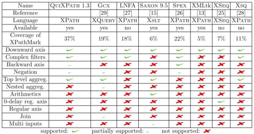
describes a deterministic eNwa. Furthermore, selection and rejection can be decided no later than when closing the start node. In this case, we can construct D such that it runs D1on all children of the start node, deterministically one by one, until a selection state is reached or the start node was closed. This can be done by adding 2 states and stack symbols to D1only, based on a recomputation trick for the stack symbol pushed at the start node by D1 [9].

The eNwa described by D = D(E) first reads the opening event of the start node, say ((a, V#_{, V}##_{)) and goes into a rejection state if there exists x ∈ V}#_such that F13 fut(x) or if V#∩ V##,= ∅. In the latter case, C will block. Otherwise, D behaves as D1 but stacks the Boolean 0 (stating that no previous child was tested successfully) instead of what D1would stack. The missing stack symbol will then be recomputed when closing the root of the child. In order to construct D alike, one needs to iterate over the head of D1, but does not have to touch the rest of D1. This can be done in time |h(D1)|. The selection states of D

are those of D1, while D introduces a new rejection state. Whenever a run of D1 goes into a rejection state of D1 (which is not a rejection state of D), then automaton D may stop any further child tests if x occurs in a set of γ and F13 fut(x), in which case D goes into its rejection state. If D reaches the closing event of the start node (that is when the Boolean 0 is popped), then D also goes into the rejection state (this is correct again since F1 contains no following axes, so that rejection of ch(F1) can be decided there). Therefore, no external stack symbol from E will ever be read by D (they may appear only after selection or rejection).

Case F = A(F1) where A ∈ {ch+, ns+, fo} or F = ch(F1) where F1 con-tains recursive axes or disjunctions. Let D1= DF1(E ∪Γnew) be the eNwa

descriptor for F1, where Γnew is the set of stack symbols that D = DF(E) in-troduces. A nondeterministic eNwa is described by D, which guesses an A-successor of the start node and runs D1starting there. There is a main run of D, which for all non-A successors of the start node goes into a skip state qskip, and which goes into a state q that generates tests for F1for potential following A-successors: For A = ch the main run goes to state q such that the next po-tential opening event is a child of the start node, and it stays in qskip for the subtrees of children of the start node. For A = ch+the main run goes and stays in state q for all descendants of the start node (no skip state qskip needed). For A = ns+ _{the main run goes to state q for all siblings to the right of start node,} and it stays in qskip for the subtree of the start node and any of the subtrees of its siblings to the right. For A = fo the main run skips the subtree of the start node and after stays in q for the rest of the stream, which is done via closing rules q−−−−−→ q for all β ∈ E. The main run of D starts tests for F(true):β 1by adding a rule q−−−→ p for each initial rule i$a%:α −−−→ p of D$a%:α # _{with i ∈ Q}

I of D#. This main run will continue until:

- either x occurs in a set of γ and F13 fut(x), in which case D goes into a rejection state, or

- the closing event of the start node of P arrives (for A = ch and A = ch+), - the closing event of the parent of the start node of P arrives (for A = ns+_), - the end of the stream arrives (for A = fo), indicated by a unique top most

stack symbol.

Automaton descriptor D inherits its selection and rejection states from D1. Note that here it matters again that a candidate can be rejected only if all runs of D on this candidate go into a rejection state.

Case F = B(F1). Without loss of generality, let B = L1& . . . &Lm&x1& . . . &xn where n+m ≥ 1 such that Li∈ L and xi∈ V0. Let DF1(E) be the eNwa

descrip-tor for F1. We build D from D1, by restricting all label descriptors of initial rules of D1 by B: Descriptors (E1& . . . Ek, (V1, V2), (V1#, V2#)) are replaced by (E1& . . . &Ek&L1& . . . &Lm, (V1∪ {x1, . . . , xn}, V2), (V1#, V2#)). Furthermore, in

order to obtain pseudo-completeness, we add one new rule to D for each conjunct of B and each initial state of D1going into a rejection state of D1: For 1 ≤ i ≤ m the new initial rule has label descriptor (¬Li&Li+1& . . . &Lm, (∅, ∅), (∅, ∅)), which describe the complement of L1& . . . &Lm deterministically. The initial rule for 1 ≤ i ≤ n has label descriptor (true, (∅, {xi}), (∅, ∅)) describing all vari-able subsets that do not contain xi. D inherits selection and rejection states from D1.

Case F = Ow. The eNwa descriptor D for Ow has to compute the concate-nation of all strings of text nodes contained in the subtree of the start node, and has to compare it to w with respect to O. This is done by creation of a deterministic finite state automaton B that accepts all strings w# _{such that} (w#_{, w) is in the relation induced by O. The idea is that D runs automaton} B on all strings of text nodes in the subtree of the start node. D maintains a copy of states of B, called copy states. D’s main run r remains in copy states of B whenever not reading strings of text nodes of the subtree of the start node, while r switches to corresponding states of B at text nodes. The main run starts in the initial copy state of B and stays there until the first text node arrives at which it changes to the initial state of B. The string of the text node is consumed by B, while reaching some state q which is not necessarily a final state of B. At the corresponding closing event of the text node, the main run goes into the corresponding copy state qcopyfor q and stays there until the next text node arrives, where r continues as before. The main run continues until the closing event of the start node, where Ow can be decided. Whenever B blocks, the main run moves into a rejection state, and whenever a final state of B is reached, it moves into a selection state.

Case F = true. The eNwa descriptor D for true has five plus 2|E| rules with label descriptor (true, (∅, ∅), (∅, ∅)): one opening initial rule to a selection state, opening and closing rules looping in the selection and the rejection state, and 2|E| closing rules to close the stream in the selection and rejection state. Proposition 6 (Correctness). Let E be a set of “external” stack symbols, n ≥ 0, S ∈ En_{, F an Fxp formula with variables in a finite set V ⊆ V}

0, and D = DF(E) be the constructed eNwa. Then

LS(DF(E)) = Can(Ln(F ))

The proof is straightforward by induction on the structure of Fxp-formulas, and therefore deferred to Appendix B.

Definition 7. We call an Fxp formula determinization free if it does not con-tain any disjunction or any axis from ch+, ns+_{, and fo below a negation.}

For the complexity analysis of our compiler, we will need to assume that the input Fxp formula is simple, in that all label subformulas are of one of the following three forms: B(Ow), B(A(F )) or B(true). We can transform all Fxpformulas into equivalent simple Fxp formulas by applying the rewrite rule

B(F ) → B(true) ∧ F everywhere. This procedure, however, would increase the conjunction width, on which the efficiency of our compiler depends. Instead, we will assume that the input formulas is simply labeled in the following sense. Definition 8. We call an occurrence of an operator in a formula labeled if it has some ancestor, which is a label formula B but without having any axis A in between. We call a formula simply labeled if it does not contain any labeled disjunctions and negations.

Lemma 9. Any simply labeled Fxp formula can be transformed into a simple Fxpformula with the same conjunction width in linear time.

Proof. We apply the following two rewrite rules exhaustively in a bottom-up manner. This can be done in linear time since no subformulas are copied, and it does not affect the number of conjunctions.

B(F ∧ F#_{) → B(F ) ∧ F}# B(B#_{(F )) → B&B}#_{(F )}

Both rules preserve simple labeling, since whenever one of them applies, all unlabeled disjunctions and negations of F and F# _{must be located below some} axis. Therefore, they will remain unlabeled. If none of these rules applies any more, the resulting Fxp formula is simple: subformulas B(F ∧ F#_{) and} B(B#_{(F )) would be rewritten, B(F ∨ F}#_{) and B(¬(F )) are excluded since not} simply labeled, and all other three possible forms B(true), B(A(F )) and B(Ow) are simple.

Lemma 10 (Size of automaton descriptor). There exists a constant c#such that for any Fxp-formula F , that is determinization free and simply labeled, and for any finite set E of external stack symbols: |DF(E)| ≤ (|F |(c#+ 2|E|))w(F )+1. Proof. By Lemma 9 we can make F simple in a preprocessing step in linear time without changing the conjunction width w (F ). For the treatment of re-cursive axis ch+, ns+_{, and fo, we need nondeterministic automata with multiple} initial rules. If we always had a single initial rule, then the proof of the lemma was straightforward. With multiple initial rules, we need an amortized cost analysis. Therefore, we define the amortized size of an eNwa descriptor D by AS (D) = |D| + |init(D)| where |D| is the size of D and init(D) the set of initial rules of D, i.e. rules that depart an initial state. With the constant c#_{= 7, we} can show for all determinization free Fxp formulas F that:

AS (DF(E)) ≤ (|F |(c#+ 2|E|))w(F )+1

The lemma will then follow from |DF(E)| ≤ AS (DF(E)). The proof is by induction on the structure of F . Let D = DF(E). Let E# be the extension of E and F1 and possibly F2 the subformulas of F , such that D was constructed from D1= DF1(E

#_{) and possibly D}

2= DF2(E

#_{). We write ω, ω}

respective conjunction widths of w (F ), w (F1), and w (F2), and I, I1 and I2for the number of initial rules of D, D1, and respectively D2.

Case F = F1∧ F2. The eNwa descriptor D is the product D1 and D2 where E = E#_{. Hence |D| = |D}

1| |D2| and I = I1 I2, so that: AS (D) ≤ AS (D1) AS (D2)

≤ (|F1|(c#+ 2|E|))ω1+1 (|F2|(c#+ 2|E|))ω2+1 (ind. hypo.) ≤ (|F |(c#_{+ 2|E|))}ω1+1· (|F |(c#_{+ 2|E|))}ω2+1

= (|F |(c#_{+ 2|E|))}ω1+ω2+2

= (|F |(c#_{+ 2|E|))}ω+1

Case F = F1∨F2. The eNwa descriptor D is the union of the eNwa descriptors D1and D2where |E| = |E|#, so |D| = |D1| + |D2| and I = I1+ I2. It follows that AS (D) = AS (D1) + AS (D2) and thus smaller than in the case of conjunction. Case F = ¬F1. Since F is determinization free, D1 describes a deterministic automaton, which furthermore can never get stuck, so that we only need to swap rejection and selection states of D1 in order to obtain D. Hence, by induction hypothesis: AS (D) = AS (D1) ≤ (|F1|(c#+ 2|E|))ω1+1≤ (|F |(c#+ 2|E|))ω+1 Case F = ch(F1) where F1 contains neither recursive axes nor dis-junctions. Since F1 contains no nondeterministic constructs, the automaton described by D1 will be deterministic. The eNwa described by D will thus run the eNwa described by D1(where E = E#) on all children of the marked node, until one of these runs succeeds. The rules of the head of D1 are rewritten for recomputing the stack symbols that D1 used at the roots of all children of the marked node, but the number of rules is not increased thereby. In addition, c# _{= 7 new rules were added for the treatment of the marked node. Therefore,} |D| = |D1| + c#. The size of the head of D is smaller than that of D1. Hence, AS (D) ≤ c#_{+ AS (D}

1) ≤ c#+ (|F1|(c#+ 2|E|))ω1+1≤ (|F |(c#+ 2|E|))ω+1. Case F = A(F1) where A ∈ {ch+, ns+, fo} or F = ch(F1) where F1 con-tains recursive axes or disjunctions. Now E# _{is obtained by E by adding} at most c# new stack symbols. The eNwa descriptor D has a generator state, from which it starts all initial rules I1 of D1, when being at an A-successor of the marked node. For A = fo maximum |E| rules are added in order to find all following nodes in any future. In addition, c# _{= 7 new rules were added for the} treatment of the main run of D. Thus, |D| ≤ |D1| + I1+ c#+ |E|, so that:

AS (D) = |D1| + I1+ c#+ |E| = AS (D1) + c#+ |E|

≤ (|F1|(c#+ 2|E|))ω1+1+ c#+ |E| (ind. hypo.) ≤ ((|F1| + 1)(c#+ 2|E|))ω1+1

= (|F |(c#_{+ 2|E|))}ω+1

Case F = B(F1). Since F is simply labeled, F1 has the form A(F2) or Ow or true. Hence, descriptor D1 for F1 has only one initial state. The size |D| of the eNwa descriptor D is the size of D1, plus |B| opening rules to the

initial state of D1, with which the complement of B is described (for pseudo-completeness). Hence |D| = |D1| + |B| and the number of initial rules I of D is I1+ |B|. Therefore AS (D) = |D1| + |B| + I = AS (D1) − I1+ |B| + I1+ |B| ≤ (|F1|(c#+2|E|))ω1+1+2|B| ≤ (|F |(c#+2|E|))ω+1, since 2 ≤ c#and |F | = |F1|+|B|. Case F = Ow. The size of D is the sum of at most 3 · |w| many rules for the finite state automaton B (that accepts all strings w# _{such that (w}#_{, w) is in the} relation induced by O), 3 · |w| many rules for moving in and out of copy states of B as described above, and at most c# _{many rules for the treatment of Ds} main run. In addition D needs 2|E| rules to close the stream in selection and rejection states. Hence the size of D is smaller or equal to 6|w| + c#_{+ 2|E|, while} the head of D is constant and can be bounded by c#_{. As |F | = |w| it follows} that AS (D) ≤ (|F |(c#_{+ 2|E|))}ω+1_.

Case F = true. The size |D| of the eNwa descriptor D for true is 5 and contains 2|E| many rules to close the stream. D’s amortized size is thereby smaller than (|F |(c#_{+ 2|E|))}ω+1_.

Theorem 11 (Compilation time). There exist c, c# _{> 0 such that for any} determinization free and simply labeled Fxp-formula F and any finite set E of external stack symbols, the time to compute the eNwa descriptor DF(E) is at most 2c(|F |(c#_{+ 2|E|))}w(F )+1_.

Proof. We fix a set E and constants c1 = 2, c# = 7 and c = c1+ c# = 9. We again need an amortized analysis. We define the amortized time of an eNwa descriptor D = DF(E) constructed by our algorithm as follows, where T (D) is the construction time:

AT (D) = T (D) + |h(D)| + |E|

The proof is by induction on the structure of Fxp formulas F , under the as-sumption that they are determinization free and simply labeled. Let F1 and possibly F2be the arguments of the top-level operator of F , and Di= DFi(E

#₎ be the subautomata from which D was constructed. We will also write H for |h(D)|, Hi for |h(Di)|, and similarly T for T (D), Ti for T (Di).

Case F = F1∧ F2. The time to compute an eNwa descriptor D = DF(E) for the product F is the sum of the times for computing the eNwa descriptors D1= DF1(E) and D2= DF2(E), plus the time to compute eNwa descriptor D

for F , which can be done in time c1· |D1| · |D2|. Hence AT (D) = T1+ T2+ c1|D1| |D2| + H + |E| ≤ AT (D1) + AT (D2) + c1 |D1| |D2| + H ≤ AT (D1) + AT (D2) + (c1+ 1) |D1| |D2| ≤ 2c (|F1|(c#+ 2|E|))ω1+1+ 2c (|F2|(c#+ 2|E|))ω2+1 +(c1+ 1) |D1| |D2| ≤ 2c ((|F1|(c#+ 2|E|))ω1+1+ (|F2|(c#+ 2|E|))ω2+1 (c1+ 1 ≤ c) +|D1| |D2|)

≤ 2c ((|F1|(c#+ 2|E|))ω1+1+ (|F2|(c#+ 2|E|))ω2+1 (Lemma 10) +(|F1|(c#+ 2|E|))ω1+1) (|F2|(c#+ 2|E|))ω2+1

≤ 2c ((|F1| + |F2|)(c#+ 2|E|))ω1+ω2+2 (am+ bn+ ambn≤ (a + b)m+n) ≤ 2c (|F |(c#_{+ 2|E|))}ω+1

Case F = F1∨ F2. The time to compute an eNwa descriptor D is the sum of the times to compute D1 and D2. The size of the head of D is the sum of the head of D1and the head of D2. Hence

AT (D) = T + H + |E| = T1+ T2+ H + |E| =

= AT (D1) − H1− |E| + AT (D2) − H2− |E| + H + |E| ≤ AT (D1) + AT (D2)

and thus smaller than in the case of conjunction.

Case F = ¬F1. Since F is determinization free, D1 describes a deterministic automaton, which furthermore can never get stuck, so that we only need to swap rejection and selection states of D1 in order to obtain D. Hence, by induction hypothesis: AT (D) = AT (D1) ≤ 2c(|F1|(c#+ 2|E|))ω1+1≤ 2c(|F |(c#+ 2|E|))ω+1 Case F = ch(F1) where F1 contains neither recursive axes nor dis-junctions. Since F1 contains no nondeterministic constructs, the automaton described by D1 will be deterministic. The time to compute D is the time to compute D1 (where E = E#), plus the time to rewrite the head of D1 for the recomputation of stack symbols pushed at root of the children of the marked node. In addition D takes time 2|E| to delete closing stream rules for the rejec-tion state of D1 and to add these to the new rejection state of D1, and time at most c# _{to add at most c}# _{new rules for the treatment of the marked node. The} head of D contains only 5 rules. Hence

AT (D) = AT (D1) − H1− |E| + H1+ 2|E| + c#+ H + |E| = AT (D1) + 2|E| + c#+ 5

≤ 2c(|F1|(c#+ 2|E|))ω1+1+ 2|E| + c#+ 5 (ind. hypo.)

≤ 2c((|F1| + 1)(c#+ 2|E|))ω1+1 5 ≤ c

= 2c(|F |(c#+ 2|E|))ω+1

Case F = A(F1) where A ∈ {ch+, ns+, fo} or F = ch(F1) where F1 con-tains recursive axes or disjunctions. The time to compute D is the time to compute D1where E#is obtained from E by adding at most c#new stack symbols.

Furthermore D needs time to compute I1many rules for starting the test for F1 from Ds generator state, plus |E| closing rules to reach all following nodes of the stream for the case that A = fo, plus at most c# _{rules for the treatment of the} main run. The head H = H1− I1+ 2, as the head of D contains all closing rules of the head of D1, but none of the initial rules belonging to the head of D1, such that D needs two new initial rules. Therefore AT (D) = T (D) + h(D) + |E| =

AT (D) = T1+ I1+ |E| + c#+ h(D) + |E|

= AT (D1) − H1− |E| + I1+ |E| + c#+ H1− I1+ 2 + |E| = AT (D1) + c#+ 2 + |E|

and thus smaller than in the case of F = ch(F1) where F1 contains no nonde-terministic constructs.

Case F = B(F1). Since we assumed that F is simply labeled, it follows that F1 is either a comparison Ow, an axis A(F2), or true. In all cases, the eNwa descriptor D1for F1has only one initial state, and its head H1is of size at most c#_{. Therefore the time T for computing D is the time to compute D}

1, plus the time to intersect label properties and variable restriction in B with the label descriptors of initial rules of D1 (of which there are at most H1 many), plus the time to add an opening rule for the initial state of D1 to some rejection state of D1 to describe the complement of B. The head of D contains all rules from the head of D1, plus |B| rules for the initial state in order to maintain pseudo-completeness. Hence

AT (D) = T + H + |E| = T1+ c#+ |B| + H + |E|

= AT (D1) − H1− |E| + c#+ |B| + H1+ |B| + |E| = AT (D1) + c#+ 2|B|

≤ 2c(|F1|(c#+ 2|E|))ω1+1+ c#+ 2|B| (ind. hypo.)

≤ 2c(|F |(c#_{+ 2|E|))}ω1+1 _{|F | = |F}

1| + |B| Case F = Ow. The time to compute D is the time to compute at most 3 · |w| many rules for the finite state automaton B (that accepts all strings w# _such that (w#_{, w) is in the relation induced by O), the time to compute 3 · |w| many} rules for moving in and out of copy states of B as described above, the time to compute at most c# _{many rules for the treatment of Ds main run, plus 2|E|} rules to close the stream in selection and rejection states. D’s head contains only four rules. With |F | = |w| the amortized time to compute D is therefore at most 6|w| + c#+ 2|E| + 4 + |E| ≤ 2c(|F |(c#+ 2|E|))ω+1.

Case F = true. The time to compute D is the time to compute the 5+2|E| many rules. The head of D has size 3 (initial rule plus 2 closing rules in for the selection and rejection state). D’s amortized time is therefore 5 + 2|E| + 3 + |E| = 8 + 3|E|, which is smaller than 2c(|F |(c#_{+ 2|E|))}ω+1_.

6. Early Query Answering

We show how to use eNwa descriptors for evaluating monadic queries on Xmlstreams. The main idea is to generate on the fly all possible answer candi-dates, and to run the described eNwa on all of them in parallel in a streaming

manner. The nondeterminism and the automata descriptors are resolved by on-the-fly instantiation and determinization. We then improve this streaming algorithm in an important manner, so that the stacks and states of the runs of multiple answer candidates in the same state may be shared.

6.1. On-the-fly Instantiation and Determinization

Let D be a descriptor of an eNwa E# _{that defines a monadic query, i.e.,} with tag alphabet {a, ax_{| a ∈ Σ} where x is a fixed variable. We are interested} in running the determinization E of E#_{. This can be done while generating} the needed part of E from D on the fly (and thus without ever constructing E#_{). At any time point, we store the subset of the states and transitions of} E that were used before. If a missing transition rule is needed for some state {(q1, q#1), . . . , (qk, qk#)} of E and some label l then for each 1 ≤ i ≤ k one com-putes transitions of D from state qithat describe label l (if not already computed once). These transition rules are then used to compute the result state of E by applying the determinization procedure. It should be noticed that each tran-sition of E can be computed in polynomial time (but not in linear time). For example, to compute a missing closing transition of the deterministic automa-ton by on-the-fly determinization, our algorithm needs time O(|Q|4_{· |Σ|), where} Q are the states of E# _{(see Appendix A). Recall also that the states of E are} sets of pairs of states of E#_{. For efficiency reasons, we will substitute such sets} by integers, so that the known transitions of E can be executed as efficiently as if a deterministic eNwa E# _{was given at beforehand. Therefore, we can safely} separate the aspects of on-the-fly instantiation and determinization from what follows.

6.2. Streaming Algorithm for Deterministic ENWAs

We present a streaming algorithm that answers monadic queries defined by a deterministic eNwas E in an early manner. This algorithm can then be lifted to eNwadescriptors by on-the-fly determinization and instantiation, as explained above. We will also assume that the deterministic eNwa E is pseudo-complete, so that it has a unique complete run on any document.

Buffering Possibly Alive Candidates. Suppose that we are given a stream con-taining a nested word of some data tree, and that we want to compute the answers of the query defined by E on this data tree in an early manner. That is, we have to find all nodes of the data tree that can be annotated by x, so that E can run successfully on the annotated data tree. At any event e of the stream, our algorithm maintains a finite set of candidates in a so-called buffer. A candidate is a triple that contains a value for x, a state of E that is neither a selection nor a rejection state, and a stack of E. The value of x can either be a node opened before the current event e, or “unknown” which we denote by •. At the start event, there exists only a single candidate in the buffer, which is (•, q0, ⊥) where q0 is the unique initial state of E and ⊥ the empty stack. At any later event, there will be at most one candidate containing the •.