Comparative Analysis of Robust Design Methods
by
Jagmeet Singh
B. Tech., Mechanical Engineering
Indian Institute of Technology at Kanpur, 2001
S.M., Mechanical Engineering
Massachusetts Institute of Technology, 2003
Submitted to the Department of Mechanical Engineering
In Partial Fulfillment of the Requirements for the Degree of
DOCTOR OF PHILOSOPHY
at the
MASSACHUSETTS INSTITUTE OF TECHNOLOGY
June 2006
( 2006 Massachusetts Institute of Technology
All rights reserved
Signature of Author
Department of Mechanical Engineering
py-p 2006
Certified by
D
Fre
Daniel . Frey
Assistant Professor, Department of Mechanical Engineering and Engineering Systems
Thesis Supervisor
Accepted by.
MASSACHUSETTS INSTITUTE, OF TECHNOLOGYJUL 1
4
2006
Lallit Anand
Chairman, Department Committee on Graduate Studies
Comparative Analysis of Robust Design Methods
by
Jagmeet Singh
Submitted to Department of Mechanical Engineering
on May
5,
2006 in partial fulfillment of the
requirements for the degree of Doctor of Philosophy in
Mechanical Engineering
Abstract
Robust parameter design is an engineering methodology intended as a cost effective
approach to improve the quality of products, processes and systems. Control factors are
those system parameters that can be easily controlled and manipulated. Noise factors are
those system parameters that are difficult and/or costly to control and are presumed
uncontrollable. Robust parameter design involves choosing optimal levels of the
controllable factors in order to obtain a target or optimal response with minimal variation.
Noise factors bring variability into the system, thus affecting the response. The aim is to
properly choose the levels of control factors so that the process is robust or insensitive to
the variation caused by noise factors. Robust parameter design methods are used to make
systems more reliable and robust to incoming variations in environmental effects,
manufacturing processes and customer usage patterns. However, robust design can
become expensive, time consuming, and/or resource intensive. Thus research that makes
robust design less resource intensive and requires less number of experimental runs is of
great value. Robust design methodology can be expressed as multi-response optimization
problem. The objective functions of the problem being: maximizing reliability and
robustness of systems, minimizing the information and/or resources required for robust
design methodology, and minimizing the number of experimental runs needed. This
thesis discusses various noise factor strategies which aim to reduce number of
experimental runs needed to improve quality of system. Compound Noise and
Take-The-Best-Few Noise Factors Strategy are such noise factor strategies which reduce
experimental effort needed to improve reliability of systems. Compound Noise is made
by combing all the different noise factors together, irrespective of the number of noise
factors. But such a noise strategy works only for the systems which show effect sparsity.
To apply the Take-The-Best-Few Noise Factors Strategy most important noise factors in
system's noise factor space are found. Noise factors having significant impact on system
response variation are considered important. Once the important noise factors are
identified, they are kept independent in the noise factor array. By selecting the few most
important noise factors for a given system, run size of experiment is minimized.
Take-The-Best-Few Noise Factors Strategy is very effective for all kinds of systems
irrespective of their effect sparsity. Generally Take-The-Best-Few Noise Factors Strategy
achieves nearly 80% of the possible improvement for all systems. This thesis also tries to
find the influence of correlation and variance of induced noise on quality of system. For
systems that do not contain any significant three-factor interactions correlation among
noise factors can be neglected. Hence amount of information needed to improve the
quality of systems is reduced.
Thesis Supervisor: Daniel D. Frey
Title: Robert N. Noyce Assistant Professor, Department of Mechanical Engineering &
Engineering Systems
Committee Member: Daniel E. Whitney
Title: Senior Research Scientist, Center for Technology, Policy and Industrial
Development and Department of Mechanical Engineering, Senior Lecturer in
Engineering Systems
Committee Member: Warren P Seering
Acknowledgements
I offer prayer of thanks to GOD for giving me this wonderful opportunity to do research
in one of the premier institutes. I would like to thank my thesis advisor Dan Frey. I am always short of words for his mentorship, support, guidance, patience and integrity. I have leamt a lot from him in both research and life. He is one of best advisors that one could have asked for in research. It was for him that I truly enjoyed my PhD research and was always excited about it through out my duration of PhD.
Dan Whitney and Warren Seering are the best committee members to have. Their keen observations and tremendous experience helped me a great deal in shaping path of my research. They helped me a lot in putting my research results in perspective. I have been leaming from them since the day I joined MIT. I again find myself short of words to thank both of them for their support, guidance, mentorship and blessings. I would also like to thanks Nathan Soderborg, Joe Saleh and Ford-MIT Research Alliance for
supporting this research.
My grandparents, parents, Mr. Yashpal Singh and Mrs. Surjeet Kaur and sister, Jaideep
Kaur provided me with support all throughout my research. And no acknowledgement is complete without mentioning Rajesh Jugulum. He is part of our research group. His reviews on research progress, his insights were very helpful in the progress of research. I would also like to thank my friends for their goodwill and support.
Table of Contents
A b s tra c t ...
3
Acknowledgements ... 5 L ist o f F ig u re s ... . 11 L is t o f T a b le s ... 15 Chapter 1: Introduction ... 19 1.1 M o tiva tio n ... . 19 1.2 Goal of Research... 20 1.3 Organization of Thesis... 21Chapter 2: Hierarchical Probability Model ... 23
2.1 Regularities in Engineering Systems ... 23
2.2 Hierarchical Probability Model ... 25
2.3 Selecting parameters for Hierarchical Probability Model ... 30
2.4 Variants of Hierarchical Probability Model... 31
2.5 Chapter Summary ... 34
Chapter 3: Compound Noise: Evaluation as a Robust Design Method ... 37
3.1 Introduction and Background... 37
3.2 Setting up of Compound Noise study ... 41
3.2.1 Generating Response Surface instances... 42
3.2.2 Algorithm to study Compound Noise... 47
3.2.3 Measures studied... 49
3.2.4 Results from Compound Noise studies... 50
3.2.5 Conclusions from Probability Model... 56
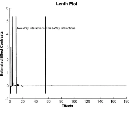
3.3.1 Lenth Plots for Case Studies
...
58
3.3.2 Results from Compound Noise Strategy on Case Studies ... 63
3.4 Effectiveness of Compound Noise in Real scenarios ... 65
3.5 Conditions for Compound Noise to be completely effective
...
69
3.5.1 Strong Hierarchy Systems ... 69
3.5.2 Weak Hierarchy Systems ... 72
3.5.3 Conclusions from Case Studies ... 76
3.6 C on clusions ... 77
3.7 Chapter Sum m ary ... 82
Chapter 4: Take-The-Best-Few Strategy: Evaluation as a Robust Design M e th o d ... 8 5 4.1 Introduction and Background ... 85
4.2 Setting up of TTBF study ... 87
4.2.1 Generating Response Surface instances... 88
4.2.2 Algorithm to study TTBF strategy ... 90
4.2.3 M easures studied ... 93
4.2.4 Results from TTBF Strategy studies... 94
4.2.5 Conclusions from Probability Model ... 99
4.3 Comparison of TTBF strategy and Compound Noise strategy...100
4.4 Case Studies and effectiveness of TTBF strategy ... 104
4.4.1 Effectiveness of TTBF strategy in Real scenarios... 107
4.5 H ybrid N oise S trategy ... 109
4.6 C o n clusion s ... 111
4.7 C hap ter S um m ary ... 114
Chapter 5: Analyzing effects of correlation among and intensity of noise factors on quality of system s ... 117
5.2.2 Algorithm to evaluate noise strategies ...
130
5.2.3 M easures studied
...
133
5.2.4 Results from model-based analysis
...
133
5.2.5 Significance of results from model-based approach... 135
5.3 C a s e S tu d ies
...
136
5.3.1 Results from Case Studies... 137
5.4 C o n clus io n s
...
139
5.5 C hap ter S um m ary
...
142
Chapter 6: Conclusions and Future Work... 145
6.1 O verview of research
...
145
6.2 Algorithms to improve quality of systems
...
149
6.3 Cost-Benefit Analysis of Robust Design Methods... 155
6.4 Scope of future research...
159
R E F E R E N C E S
...
16 1
Appendices: MATLAB® and Mathcad-I1 Files
...
165
List of Figures
Figure 2.1: The hierarchy and heredity among main effects and interactions in a system with four factors A, B, C, and D. Interactions between factors are represented by letter combinations such as the two-factor interaction AC. The font size represents the size of the effect... 25
Figure 3.1: Algorithm used to evaluate Compound Noise Strategies... 48
Figure 3.2: Improvement Ratio: Ratio of Realized Reduction to Maximum R eduction possible... 50
Figure 3.3: Median Improvement Ratio verses Effect Density for Strong Hierarchy Response Surface Instances... 54
Figure 3.4: Median Improvement Ratio verses Effect Density for Weak Hierarchy Response Surface Instances... 55
Figure 3.5: Median Improvement Ratio verses Effect Density for both Strong and Weak Hierarchy Response Surface Instances... 56
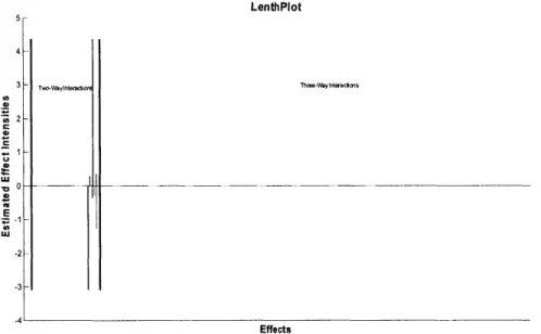
Figure 3.6: Lenth Plot of Effect Coefficients for Op Amp, Phadke (1989)... 59
Figure 3.7: Lenth Plot of Effect Coefficients for Passive Neuron Model, Tawfik
and D urand (1994)... 60
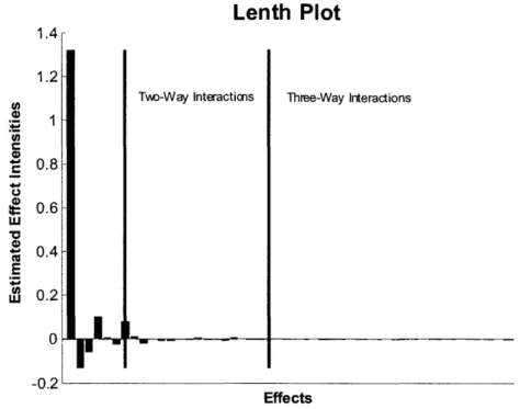
Figure 3.8: Lenth Plot of Effect Coefficients for Journal Bearing: Half Sommerfeld Solution, H am rock, et al. (2004)... 61
Figure 3.9: Lenth Plot of Effect Coefficients for CSTR, Kalagnanam and Diwekar (199 7)... 62
Figure 3.10: Lenth Plot of Effect Coefficients for Temperature Control Circuit,
Phadke (1989)... 62
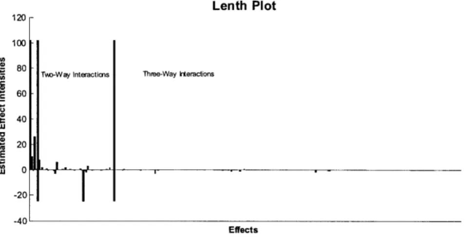
Figure 3.11: Lenth Plot of Effect Coefficients for Slider Crank, Gao, et al. (1998)... 63
Figure 3.12: Median Improvement Ratio verses Effect Density for Strong and Weak Hierarchy Response Surface Instances and Six Case Studies... 79
Figure 3.13: Suggested procedure for Compound Noise in Robust Design... 82
Figure 4.1: Algorithm used to evaluate TTBF strategy... 92
Figure 4.2: Median Improvement Ratio verses Effect Density for Strong Hierarchy Response Surface Instances... 97
Figure 4.3: Median Improvement Ratio verses Effect Density for Weak Hierarchy R eponse Surface Instances ... 98
Figure 4.4: Median Improvement Ratio verses Effect Density for both Strong and Weak Hierarchy Response Surface Instances... 99
Figure 4.5: Median Improvement Ratio verses Effect Density for Strong and Weak Hierarchy Response Surface Instances and Six Case Studies... 112
Figure 5.2: Algorithm used to evaluate Noise Strategies...
Figure 5.3: Flowchart to reduce information needed to implement Robust Design
M ethodology ... 14 1
Figure 6.1: Suggested procedure for TTBF Strategy and Compound Noise in R obu st D esign ... 15 1
Figure 6.2: Flowchart to reduce information needed to implement Robust Design
M ethodolo gy ... 154
Figure 6.3: Cost-Benefit Analysis of Robust Design Methods for reducing experim ental run s... 156
Figure 6.4: Cost-Benefit Analysis of Robust Design Methods for minimizing information regarding noise factor space... 158
List of Tables
Table 2.1: Parameters for Hierarchical Probability Model...
Table 2.2: Additional parameters for Hierarchical Probability Model...
Table 2.3: Parameters for Variants of Hierarchical Probability Model...
Table 3.1: Hierarchical Probability Model Parameters used for Strong Hierarchy R esponse Surface instances...
Table 3.2: Hierarchical Probability Model Parameters used for Weak Hierarchy R esponse Surface instances...
Table 3.3: Hierarchical Probability Model Parameters used for Strong Hierarchy Response Surface instances, reflecting effect spars ity...
Table 3.4: Hierarchical Probability Model Parameters used for Weak Hierarchy Response Surface instances, reflecting effect sparsity...
T ab le 3 .5 : M easure 1...
T able 3 .6 : M easure 2 ...
T able 3 .7 : M easure 3...
T ab le 3 .8 : M easure 3 ...
Table 3.10: M easure 4...
Table 3.11: Results from Full Factorial Control Factor array and Two-Level Extrem e Compound N oise...
Table 3.12: Results from Resolution III Control and Noise Factor Array...
Table 3.13: Results from Resolution III Control Factor array and Two-Level Extrem e Compound N oise...
Table 3.14: Average results from Full Factorial Control Factor array and Two-Level Simple Compound N oise Strategy...
Table 4.1: Hierarchical Probability Model Parameters used for Strong Hierarchy Response Surface instances...
Table 4.2: Hierarchical Probability Model Parameters used for Weak Hierarchy Respone Surface instances ...
Table 4.3: M easure 1... Table 4.4: M easure 2... Table 4.5: M easure 3... Table 4.6: M easure 3... Table 4.7: M easure 4... 53
T ab le 4 .9 : M easure 1... T able 4 .10 : M easure 2 ... T able 4 .11: M easure 3 ... T able 4 .12 : M easure 3 ... T able 4 .13: M easure 4 ... T able 4 .14 : M easure 4 ...
Table 4.15: Results from Full Factorial Control Factor array and TTBF strategy...
Table 4.16: Results from Resolution III Control and Noise Factor Array...
Table 4.17: Results from Resolution III Control Factor array and TTBF Strategy....
Table 5.1: Parameters for Variants of Hierarchical Probability Model...
Table 5.2: Median fraction of the maximum possible improvement attained in hierarchical probability response surface instances...
Table 5.3: Percentage of hierarchical probability response surface instances in which optimum control factor settings were attained...
Table 5.4: Median fraction of the maximum improvement attained in case study sim u latio n s...
Table 5.5: Percentage of case study simulations in which optimum control factor settin gs w ere attained ...
101 101 102 102 102 103 105 108 108 129 134 134 137 138
Chapter 1: Introduction
1.1 Motivation
Robust parameter design is an engineering methodology intended as a cost effective approach to improve the quality of products, processes and systems, Taguchi (1987), Robinson et al. (2004). Taguchi (1987) proposed that inputs to any system can be classified as control factors and noise factors. Control factors are those system parameters that can be easily controlled and manipulated. Noise factors are those system parameters that are difficult and/or costly to control and are presumed uncontrollable. Robust parameter design involves choosing optimal levels of the controllable factors in order to obtain a target or optimal response with minimal variation. The challenge arises in obtaining optimal response due to the influence of the uncontrollable noise factors. Noise factors bring variability into the system, thus affecting the response. The aim is to properly choose the levels of control factors so that the process is robust or insensitive to the variation caused by noise factors.
Robust parameter design is among one of the most important developments in systems engineering in 20th century, Clausing and Frey (2005). These methods seemed to have accounted for a significant part of quality differential that made Japanese manufacturing dominant during 1970s. Robust parameter design enables in smoother system integration, faster transition to production, and higher field reliability.
Taguchi (1987) also proposed techniques of experimental design to identify the settings of control factors that would achieve robust performance of systems. He used orthogonal designs where an orthogonal array involving control factors ('inner array') is crossed with an orthogonal array involving noise factors ('outer array'). The response of the systems' at each setting of control factors were treated as replicates for the formulation of a measure that would be indicative of both the mean and variance of response. One of the weaknesses of these crossed array experiments is that they tend to require large number of experimental runs.
1.2 Goal of Research
Robust parameter design methods are used to make systems more reliable and robust to incoming variations in environmental effects, manufacturing processes and customer usage patterns. However, robust design can become expensive, time consuming, and/or resource intensive. Thus research that makes robust design less resource intensive and requires less number of experimental runs is of great value. Robust design methodology can be expressed as multi-response optimization problem. The objective functions of the problem being: maximizing reliability and robustness of systems, minimizing the information and/or resources required for robust design methodology, and minimizing the number of experimental runs needed. We will present noise strategies for robust design methods which would reduce the amount of experimental effort needed and information
1.3 Organization of Thesis
The thesis will first present simplest of the noise strategy which minimizes amount of experimental effort needed. Then it will suggest some alternative, useful and more efficient noise factor strategies. Chapter 2 will discuss the formulation of hierarchical probability model. This will form the basis to compare different robust design methods statistically. First the regularities exhibited by engineering systems will be discussed. Next those regularities will be put in a mathematical format. The mathematical formulation will be used to generate response surface instances to analyze different robust design methods. We will also discuss about selection of various parameters for hierarchical probability model.
Chapter 3 will introduce Compound Noise. Compound Noise is very effective as a robust design strategy on the systems which show effect sparsity. We will run two formulations of compound noise on response surface instances generated using strong and weak hierarchical probability model. Next these formulations of compound noise will be run on six different case studies from various engineering domains to verify conclusions from hierarchical probability model. In the end conditions for compound noise to be completely effectiveare outlined . We will also device an algorithm to use compound
noise as a robust design method.
Chapter 4 will introduce Take-The-Best-Few Noise Factor Strategy, which is very effective as a robust design strategy for all kinds of systems. We will run this noise strategy on response surface instances generated using strong and weak hierarchical
probability model and six different case studies from various engineering domains. We will also compare this noise strategy with compound noise strategy. We will propose hybrid noise strategy as amalgamation of two noise strategies. We will then device an algorithm on the use of this noise strategy and compound noise strategy as robust design methods.
Chapter 5 will explore the influence of correlation among noise factors on robust design methods. We will see the impact of correlation and variance of induced noise factors on response surface instances and six different case studies. We will see that if system does not have any significant three-factor interaction then during robust design experiments we can neglect correlation and/or exaggerate intensity of induced noise factors. We will design an algorithm for implementing correlation influence in practice.
Chapter 6 will summarize the key messages from this thesis. It will present cost-benefit analysis of various robust design methods and the percentage improvement each robust design method can give for a given system. This cost-benefit analysis can be used by engineers to find the maximum benefit they can get out of a robust design study based on their allocated budget. Also it outlines scope of future research in area of robust design. This will be followed by references and appendices.
Chapter 2: Hierarchical Probability Model
2.1 Regularities in Engineering Systems
Experimentation is an important activity in design on systems. Almost every existing engineering system was shaped by a process of experimentation including preliminary investigation of phenomenon, sub-system prototyping, and system verification tests. Based on experience in planning and analyzing many experiments, practitioners and researchers in system design have identified regularities in the inter-relationships among factor effects and their interactions, Wu and Hamada (2000). Hamada and Wu (1992),
Box and Meyer (1986), Chipman, Hamada and Wu (1997) and Wu and Hamada (2000)
describe these regularities in detail:
Effect Sparsity Principle - among many effects examined in any system only a small fraction of those effects are significant in system, Box and Meyer (1986). This is sometimes called the Pareto principle in Experimental Design based on analogy with the observations of the 19th century economist Vilfredo Pareto who argued that, in all countries and times, the distribution of income and wealth follows a logarithmic pattern resulting in the concentration of resources in the hands of a small number of wealthy individuals. Effect sparsity appears to be a phenomenon characterizing the knowledge of the experimenters more so than the physical or logical behavior of the system under investigation. Investigating an effect through experimentation requires an allocation of resources -- to resolve
more effects typically requires more experiments. Therefore, effect sparsity is in some sense an indication of wasted resources. If the important factor effects could be identified during planning, then those effects might be investigated exclusively, resources might be saved, and only significant effects would be revealed in the analysis.
* Hierarchical Ordering Principle - main effects are generally more significant that two factor interactions, two-factor interactions are generally more significant than three-factor interactions, and so on, Hamada and Wu (1992). Effects of same order are likely to have same significance level. This principle is also sometimes referred as "hierarchy". Effect hierarchy is illustrated in figure 2.1 for a system with four factors A, B, C and D. Figure 2. lillustrates a case in which hierarchy is not strict - for example, that some interactions (such as the two-factor interaction
Figure 2.1: The hierarchy and heredity among main effects and interactions in a system with four
factors A, B, C, and D. Interactions between factors are represented by letter combinations such as
the two-factor interaction A C. The font size represents the size of the effect.
Effect Heredity Principle - an interaction effect is likely to be significant when at least one of its parent factors is significant, Wu and Hamada (2000). It is also sometimes referred to as "inheritance".
2.2 Hierarchical Probability Model
Hierarchical probability models have been proposed as a means to analyze the results of experiments with complex aliasing patterns. In any system main effects and interaction effects present are of interest. There is also a need to predict the relative importance and
relationship among these effects. Chipman, Hamada and Wu (1997) have expressed these properties in mathematical form in a hierarchical prior probability model. The hierarchical probability model proposed by Chipman, Hamada and Wu (1997) has been extended here to enable evaluation of noise strategies in robust design. The model includes both control and noise factors since they are both needed for the present purposes. The model includes two-factor interactions since control by noise interactions are required for robust design to be effective. It also includes the possibility of three-factor interactions since these have been shown to be frequently present, especially in systems with a large number of factors Li and Frey (2005) and might affect the outcomes of robust design. The details of the model are in Equations 2.1 through 2.10.
y(x,,x 2-. ,x))=$
Axi
+Z flxix +zzZ/3ixixjxk +6 (2.1xi - NID(0, w1 2 ) i E ...m (2.2) x e{,-} ie
m +1...n
(2.3)
e-
NID(0,w2 2) (2.4)N(0,s
l) if (5 = 0
r~io)
2 JFIi~j bN(O,c 2 _s 2) if '5=1 N(O,s 22) if jk =0 Jf 1ijk izkJ N(0,c2 -s2 ) if 5 ijk =1 P( =1) = p P00 Pr(S5, =1|S,S,)= Pot LPn1 fp000 Pr(jk =1|SijSk)=Pool
pollI Lpill if if if if 15+ +45 =0 45,+ '5 + 05 = 1 i j+ k2
5,+, + 5=3 (2.10)This hierarchical probability model allows any desired number of response surface instances to be created such that population of response surface instances has the desired properties of sparsity of effects, hierarchy, and inheritance. Equation 2.1 represents the measured response of the engineering system y. The independent variables x,'s are both control factors and noise factors. Control and noise factors are not distinguished in this notation except via indices. Equation 2.2 shows that the first set of x variables (xI, x2,...
(2.6) (2. 7) if if if (2. 8) S ,5 =0 i5 +5 =1 9, +S =2 (2. 9)
xm) are regarded as "noise factors" and are assumed to be normally distributed. Equation
2.3 shows that the other x independent variables (xmi, X,±2,... x,) are the "control
factors" which are assumed to be two level factors. The variable represents the pure experimental error in the observation of the response which is assumed to be normally distributed. Since the control factors are usually explored over a wide range compared to the noise factors, the parameter w, is included to set the ratio of the control factors range to the standard deviation of the noise factors. The intensity of noise factors can be changed by changing the value of parameter w1.The parameter w2 is included to set the
ratio of the standard deviation of the pure experimental error to the standard deviation of the noise factors.
The generated instance response y is assumed to be a third order polynomial in the independent variables xi's. The coefficients i's are the main effects. The coefficients i;'s
model two-way interactions including control by control, control by noise and noise by noise interactions. The coefficients ijk's model three-way interactions including control-by-control-by-control, control by control by noise, control by noise by noise and noise by noise by noise. The model originally proposed by Chipman, Wu and Hamada (1997) did not include three-way interactions. Li and Frey (2005) extended the model to included three-way interactions.
either "active" or "inactive" depending on the value (0 or 1 respectively) of their corresponding parameters i's. The parameter strength of active effects is assumed to be c times that of inactive effects. Equations 2.6 and 2.7 determine the probability density function for second order and third order coefficients respectively. In equations 2.6 and 2.7 the hierarchy principle is reflected in the fact that second order effects are only sj
times as strong (on average) as first order effects (sysl) and third order effects are only s2
times as strong as first order effects.
Equation 2.8 reflects sparsity of effects principle. There is a probability p of any main effect being active. Equation 2.9 and 2.10 enforce inheritance. The likelihood of any second order effect being active is low if no participating factor has an active main effect and is highest if all participating factors have active main effects. Thus generally one sets
pJ>po>poo and so on.
We classified systems and response surface instances based on hierarchical ordering principle. The classes are:
" Strong hierarchy systems are ones which have only main effects and two-factor
interactions active. Some small three-factor interactions might be present in such systems but they are not active.
* Weak hierarchy systems are ones which also have active three-factor
To generate a response surface instance, first the values of the probabilities of given factor effects being active (next section) are determined. Using them in equations 2.8 to 2.10, active effects for a given response surface instance are determined. Once active
effects are known equations 2.5 to 2.7 are used to find the values of P's. Equations 2.2 to 2.4 are used to find the values of control factor, noise factors and experimental error for the model. To the find the instance's response, values of xi's,
P's
and are substituted in equation 2.1.2.3
Selecting parameters for Hierarchical Probability Model
Hierarchical Probability Model has several real valued parameters which have significant effect on the inferences drawn from its use. To provide a balanced view Frey and Li (2004) in tables 2.1 and 2.2 share six different settings of parameter settings.
C Si S2 WI W2 Basic WH 10 1 1 1 1 Basic low w 10 1 1 0.1 0.1 Basic 2"d order 10 1 0 1 1 Fitted WH 15 1/3 2/3 1 1 Fitted low w 15 1/3 2/3 0.1 0.1 Fitted 2"d order 15 1/3 0 1 1
Basic WH 0.25 0.25 0.1 0 0.25 0.1 0 0
Basic low w 0.25 0.25 0.1 0 0.25 0.1 0 0
Basic 2"d order 0.25 0.25 0.1 0 N/A N/A N/A N/A
Fitted WH 0.43 0.31 0.04 0 0.17 0.08 0.02 0
Fitted low w 0.43 0.31 0.04 0 0.17 0.08 0.02 0
Fitted 2nd order 0.43 0.31 0.04 0 N/A N/A N/A N/A
Table 2.2: Additional parameters for Hierarchical Probability Model
The basic weak heredity model (basic WH) is based on the parameters used in Bayesian model selection, Chipman, Wu and Hamada (1997). Two variants were developed from this basic model. The low w variant accounts for the fact that control factors are generally explored over a wider range than noise factors. The 2"d order variant zeros out the
coefficients of all the three-factor interactions. The fitted weak heredity model (fitted WH) was developed by Frey and Li (2004) based on experimental data.
Through out this thesis several different variants of these model parameters will be used. We will also use other parameter values, different from the ones as given over here to explore some effects in greater details. This would be done specifically to study the effectiveness of Compound Noise strategy and Take-The-Best-Few strategy on systems showing effect sparsity.
2.4
Variants of Hierarchical Probability Model
To study the impact of neglecting correlation among noise factors on Robust Design Studies, some more variants of Hierarchical Probability Model were developed. In particular equation 2.2 was modified as:
Pot IIPoo Pill IPoll IPool
(2.11)
Equation 2.11 shows that the first set of m input parameters to Hierarchical Probability Model (xI, X2,..., xm) are regarded as noise factors and are assumed to be normally distributed with variance-covariance K among noise factors.
Multiple variants of the hierarchical probability model were formed by selecting different sets of model parameters as described in Table 2.3. As the column headings of Table 2.3 indicate, a key difference between the variants is the assumption concerning effect hierarchy. A Strong Hierarchy Model assumes that the only active effects in the system are main effects and two-factor interactions although small three factor interactions are present as can be seen in Equation 2.7. A Weak Hierarchy Model includes a possibility for active three-factor interactions. The values for parameters in Table 2.3 such as p11=0.2 5 and poJ=0.I are based on the Weak Heredity model proposed by Chipman,
Hamada and Wu (1997). In fact, the Strong Hierarchy model is precisely the Weak Heredity model published in that paper and used for analyzing data from experiments with complex aliasing patterns. The Weak Hierarchy model proposed here is an extension of that model to include higher order effects and therefore relies less on the assumption of hierarchy.
covariance matrix was also composed by three different methods inducing different degrees of correlation. These resulted in off-diagonal elements of the covariance matrix with different average magnitudes. Given the two model options related to the columns of Table 2.3 and the additional combinations of options due to the alternatives in the last three rows, there are 24 different model variants in all.
Table 2.3: Parameters for Variants of Hierarchical Probability Model
K is the variance-covariance matrix for the real noise factors. The modeled noise, in
response surface instance is assumed to have a covariance of an identity matrix. Thus the more different K is from an identity matrix, the more the noise strategy varies from a faithful representation of the noises the system will experience in the field.
parameters Strong Hierarchy Model Weak Hierarchy Model
(active main effects and two- (active three-factor factor interactions) interactions also included)
m 5 5 n 12 12 c 10 10 p 0.25 0.25 p11 0.25 0.25 pOI 0.1 0.1 POO 0.0 0.0 pill 0.0 0.25 Poll 0.0 0.1 poo] 0.0 0.0 POOO 0.0 0.0 7 1 or 10 1 or 10 K 1.0 or 1.75 1.0 or 1.75 K
I0.01,
0.26, or 0.47 0.01, 0.26, or 0.47 iThe on-diagonal elements of the matrix, Kii, are the variance due to each noise factor xi.
The size of these on-diagonal elements is an indication of the amplitude of the real noise factors relative to the modeled noise factors. Two options within the model are defined: one in which the real noise has the same variance as the modeled, and one in which the real noise has higher variance than the modeled.
The off-diagonal elements of the matrix, Ki;, are the covariance among noise factors xi and x;. Three options within the model are defined: one with almost no correlation (with the average absolute value of the correlation coefficients being 0.01), one with relatively mild correlation (with the average absolute value of the correlation coefficients being 0.26) and one with relatively strong correlation (with the average absolute value of the
correlation coefficients being 0.47). The matrix K was formed so as to ensure the resulting matrix was positive semi-definite while also having the desired variance and the desired degree of correlation.
2.5 Chapter Summary
In this chapter the formulation of Hierarchical Probability Model was discussed. This will form the basis to compare different robust design methods statistically. First the regularities exhibited by engineering systems were discussed. Next those regularities were put in a mathematical format. The mathematical formulation would be used to
have many variants of Hierarchical Probability Model. We discussed some of these variants.
In the next chapters some robust design methods will be discussed, which focus on reducing number of experiments done on systems and reducing amount of information required about system and still improve robustness of the system. We will use Hierarchical Probability Model as one of the basis to analyze these robust design methods.
Chapter 3: Compound Noise: Evaluation as a Robust
Design Method
3.1 Introduction and Background
In Robust Parameter Design methodology, the effect of noise (variation) is reduced by exploiting control-by-noise interactions. These control-by-noise interactions can be captured by using crossed-array approach. The control factor setting that minimizes the sensitivity of the response to noise factors is called the optimal control factor setting or the most robust setting for the system. A crossed-array approach is a combination of two orthogonal arrays, one of control factors and other of noise factors. Exploiting control-by-noise interactions is just the beginning of reducing sensitivity of the response. For systems that have active three-factor interactions, control-by-control-by-noise and control-by-noise-by-noise interactions can also be utilized to reduce the sensitivity of system's response. But as the complexity of the system increases, use of full factorial control and noise factor arrays becomes prohibitively expensive. As an attempt to reduce the run size of this crossed-array approach, Taguchi (1987) proposed a compound noise factor technique. A compound noise factor is typically formed by combining all the noise factors of a system into a single factor, which is used instead of noise array.
When we know which noise factor levels cause the output to become large or small they are compounded so as to obtain one factor with two or three levels. On doing this, our
noise factors become a single compounded factor, no matter how many factors are involved. Taguchi (1987) and Phadke (1989) outlined conditions on the use and formulation of compound noise. Noise factors can be combined into a single compound factor based on their directionality on the response. Directionality of effects of noise factors on the response can be found by running small number of experiments. Phadke (1989) showed how to construct a compound noise factor using the results from the
Operational Amplifier and Temperature Control Circuit.
Du, et al. (2003, 2004) used percentile performance difference of the system to construct compound noise. This method is applicable for systems which show unimodal response characteristics. The compound noise formed this way also carries information about sensitivity of system's response to noise variables. In this thesis compound noise will be formed by the algorithm given by Phadke (1989). We will determine directionality of the effects of noise factors on the system's response and will combine noise factors based on their directionality.
Hou (2002) studied the conditions that will make compound noise yield robust setting for systems. Hou said "extreme settings should exist for compound noise to work". We will later find that compound noise can be effective even when extreme settings do not exist. The conditions mentioned in "Compound Noise Factor Theory" turn out to be the sufficient conditions. In later sections the analysis will be extended to determine
extend the formulation to systems which can have active effects up to three-factor interactions.
Compound Noise can be considered an extension of supersaturated designs (SSD). This concept initially originated with a paper by Satterthwaite (1959). SSDs were assumed to offer a potentially useful way to investigate many factors with few experiments. In some SSDs the number of factors being investigated may exceed the number of experiments by a large factor. Holcomb, et al. (2002) discusses the construction and evaluation of SSDs. Holcomb, et al. (2003) outlines the analysis of SSDs. Compound Noise is an unbalanced SSD. Allen and Bernshteyn (2003) discuss the advantages of unbalanced SSDs in terms
of performance and affordability. Heyden, et al. (2000) argues SSDs can be used to estimate variance of response, which can be used as a measure of robustness rather than using it to find main effects. S SDs "do not allow estimation of the effects of the individual
factors because of confounding between the main effects". But "estimation of the separate factor effects is not necessarily required" in improving robustness. Using
compound noise as a robust design method we try to estimate robustness of the system at a given control factor setting. The setting which improves this estimate is taken as the predicted robust setting.
The main aim of this chapter is to explore the effectiveness of compound noise as a robust design method. We will first look at the effectiveness of compound noise strategy on response surface instances generated using Hierarchical Probability Model, Li and Frey (2005). Two different kinds of response surface instances were generated. One with
only main effects and two factor interactions also called as strong hierarchy instances and other with main effects, two factor interactions and three factor interactions, also called as weak hierarchy instances.
The conclusions from compound noise studies on response surface instances from Hierarchical Probability Model were then verified by testing compound noise on six case studies from different engineering domains. The thesis also provides theoretical justification for the effectiveness of a compound noise strategy. This thesis also gives an alternative strategy to formulate a compound noise, distinctly different from Taguchi's formulation of compound noise. This new compound noise strategy requires no knowledge about noise factors effect for its formulation. The main take away of this chapter is that, Compound Noise as a Robust Design Method was very effective on the response surface instances and case studies for which only few effects accounted for significant impact on response.
The chapter is organized as: first we will describe setting up of compound noise strategy on response surface instances, measures we studied, results from compound noise studies followed by conclusions from Hierarchical Probability Model. Then compound noise strategy for six case studies from different engineering domains will be formulated. We will also study the conditions which lead to effectiveness of Compound Noise strategy. In the end conclusions and summary of the chapter will be given.
3.2 Setting up of Compound Noise study
The objective of this chapter is to see the effect of compounding noise on the prediction of optimal setting of a response surface instance generated by hierarchical probability model parameters and verify the results by case studies from various engineering domains. Here two kinds of compounding schemes were studied: simple compounding of noise factors and extreme compounding of noise factors. In the field when the direction of a system's response due to changing each of the noise factors is known, extreme compound noise can be constructed. This formulation of compound noise was originally proposed by Taguchi (1987) and Phadke (1989). We make a two-level extreme compound noise factor by combining noise factor levels in such a way that, at the lower setting of extreme compound noise all the noise factor settings give minimum response and vice versa. When there is no idea about the direction in which noise factors affect a system's response, simple compound noise is constructed. In this case noise factor levels are simply combined to form two-level simple compound noise. For example, we can select the setting of noise factors randomly to form lower-level compound noise.
To construct extreme compound noise strategy, some knowledge about effect of noise factors on system's response is needed. Hence it is in some sense more expensive to construct for a given system. But no such information is required about effect of noise factors while formulating simple compound noise strategy. Simple compound noise strategy is less resource intensive as compared to extreme compound noise strategy. We will apply both of these compound noise strategies to strong and weak hierarchy response surface instances and analyze robustness gain. We will explore the reasons behind
success or failure of compound noise application for response surface instances. The questions we want to address in this chapter are:
* Why is compound noise effective in achieving robust setting in certain cases, but
ineffective in other cases?
* How can we measure the effectiveness of a compound noise strategy?
* Do we need to know the directionality of noise factors to use compound noise? (Simple Compound Noise strategy vs. Extreme Compound Noise strategy)
3.2.1 Generating Response Surface instances
To study the effectiveness of compound noise strategy we will generate instances of response surfaces using Hierarchical Probability Model. The instances of response surfaces studied had 7 control factors and 5 noise factors. These response surfaces were generated according to a relaxed weak heredity model. The full third-order response surface equation is given by
12 12 12 12 12 12
2>*'. 212 = Z x + 3xix +ZIJ ijkXiXjXk+(
i=1 i=1 j=1 i=1 =1 k=1
j>i 1>1 k>j
In our study, we generated both strong and weak hierarchy response surface instances. The noises factors were assumed to be uncorrelated. Full factorial array was used for 7 control factors. Table 3.1 and table 3.2 give hierarchy probability model parameter values used to generate strong and weak hierarchy response surface instances respectively.
parameters values c 15 s_ 0.33 S2 0.67 W2 1 p 0.43 P11 0.31 POI 0.04 Poo 0
Table 3.1: Hierarchical Probability Model Parameters used for Strong Hierarchy Response Surface
instances parameters values C 15 s_ 0.33 S2 0.67 W2 1 P 0.43 Pi 0.31 POI 0.04 Poo 0.0 pill 0.17 Poll 0.08 poo] 0.02 POOO 0.0
Table 3.2: Hierarchical Probability Model Parameters used for Weak Hierarchy Response Surface
To gaze the impact of effect sparsity on the effectiveness of compound noise strategy, we changed parameter values for both strong and weak hierarchy response surfaces. The changed parameters are given in tables 3.3 and 3.4 for strong and weak hierarchy response surface instances respectively.
parameters values c 15 s_ 0.33 _S2 0.67 w2 1 P 0.3 pl' 0.15 P01 0.04 P00 0
Table 3.3: Hierarchical Probability Model Parameters used for Strong Hierarchy Response Surface instances, reflecting effect sparsity
parameters values c 15 s1 0.33 S2 0.25 W2 1 P 0.3 P11 0.15 POI 0.04 Poo 0.0 pill 0.03 poll 0.03 Poo] 0.02 POOO 0.0
Table 3.4: Hierarchical Probability Model Parameters used for Weak Hierarchy Response Surface instances, reflecting effect sparsity
For noise factors we defined 3 different noise strategies. First was a v noise array. This noise strategy is very close to full factorial noise factor array. Hence it will give almost perfect results for generated response surface instances. This will form a basis of comparison for compound noise strategies. Second was simple compound noise, in which noise factors settings were selected randomly to form two-level simple compound noise. Third was extreme compound noise, in which noise factors were compounded based on the sign of their effect coefficient in the response surface instance. The way simple and extreme compounded noises were formed for the 5 noise factors, is shown below, equations 3.2 and 3.3.
Simple Compounded Noise Factor levels
N1 N, N, N4 N5
[ random(sign()) ... ... ... ran
Extreme Compounded Noise Factor levels
N1 N, N, N4 N5
-]F-sign(pI)
-sign( 2) -sign(8 3)+ sign(#l) sign(#2) sign(,83)
dom(sign(/p5))j
- sign(/34)
sign(/34)
where 1's are the coefficient of noise factors for a given instance of response surface as predicted by hierarchy probability model parameters.
For each of the three noise strategies, we generated 200 response surface instances. For each instance of generated response surface, we used Monte Carlo on noise factors to find response variance at each level of full-factorial control factor array. The setting of control factors giving minimum variance of response was the optimal setting for that instance of response surface.
We analyzed each response surface instance by running a designed experiment using 3
27x
25-1different robust design crossed arrays: V (Noise Strategy 1), 2' x Simple (3.2)
(3.3) -sign(p,)
response surface under each crossed array experiment was then compared with optimal setting we got by using Monte Carlo on noise factors. In the next section we will present this algorithm in a diagrammatic manner.
3.2.2 Algorithm to study Compound Noise
The algorithm used to study noise compounding is shown in figure 3.1. The same algorithm was used to study both strong and weak hierarchy response surface instances. For each generated response surface instance, we studied three different robust design methods as outlined in previous section. Left hand side of the algorithm finds optimal setting of response surface instance, using Monte Carlo on noise factors. Right hand side of the algorithm finds optimal setting of response surface instance as predicted by a
27 25-1
chosen robust design method ( ' (Noise Strategy 1), 27 x Simple Compound Noise
strategy or 27x Extreme Compound Noise strategy). Various measures are finally compared to compute the effectiveness of a chosen robust design strategy.
- . --I
Relaxed weak heredity parameters
Generate a response surface instance; i.e. generate 3's
Use Monte Carlo on noise factors
Compute variance of response at each control
factor setting
Find control factor setting
wxith
minimum varianceRun a designed experiment based on one of the 3 robust
design noise strategies
Predict optimal control factor setting the one which gives minimum variance
of response
Find variance
g
predicted optimal setting using MoneCado on noise factors
Compare the results for a given robust design noise strategy
Repeat the process for 200 response surface instances
Compute median and inter-quartile range of percent reduction in variance and other
parameters
A
3.2.3 Measures studied
There were number of measures that were derived from the above study. The first was the percentage number of times a given noise strategy could predict the optimal control factor setting, as given by running Monte Carlo simulation at each control factor setting for each generated instance of response surface.
For the second measure we found the predicted optimal settings of the 7 individual control factors as given by a noise strategy. We compared the predicted optimal setting of each control factor with the optimal control factor setting as given by Monte Carlo simulation. We then found number of control factors out the 7, which had same setting as given by noise strategy and Monte Carlo simulation. The second measure was the mean of this number for 20instances that were generated.
For the third measure, we first found the predicted optimal control factor setting by using a given noise strategy. Then we ran Monte Carlo simulation on noise factors at that predicted optimal control factor setting and calculated the standard deviation labeled
strategy. The minimum standard deviation found by running Monte Carlo simulation at
each control factor setting is called copt. The third measure was the ratio of astrategy to (opt
for each generated instance of response surface. We studied the median and inter-quartile range of this measure for 200nstances that were generated.
For the fourth measure, we calculated the mean of the standard deviations, as given by Monte Carlo at each control factor setting. We called this mean as obase. This Gbase was
our reference. (abase - opt) is the maximum reduction that is possible in standard deviation
for a given instance of response surface. But by running a given noise strategy the realized reduction would only be (Gbase - strategy). The fourth meaure was the ratio of
realized reduction to the maximum reduction possible, i.e. ratio of (abase - strategy) to (abase - opt) for each generated instance. And we studied the median and inter-quartile range of this measure for 200instances that were generated. Figure 3.2 shows diagrammatic representation of positive improvement ratio for an instance of generated response surface. basem variance of Response strategy opt= Realized Reduction Maximum Reduction -0
Figure 3.2: Improvement Ratio: Ratio of Realized Reduction to Maximum Reduction possible
3.2.4 Results from Compound Noise studies
The results from Compound Noise studies on Strong and Weak Hierarchy response surface instances are presented from tables 3.5 to 3.10.
Percent Matching of ALL Control Factors with their Robust Setting
Strong .Weak
Strong Hierarchy Hira y Weak Hierarchy Hierarchy
response surfaces Hierarchy response surfaces resphs
(sparse effects) suspaces (sparse effects) sraesos
oise Strategy 1 72% 70% 63% 61% Simple 8% 6% 3% 3% Compoundig Extreme 10% 8% 4% 4% Compounding 1 8 4 Table 3.5: Measure 1
Percent Matching of Control Factors with their Robust Setting
Strong Hierarchy Strong Weak Hierarchy Weak
response surfaces rsp hs response surfaces rsp hs
(sparse effects) surfaces (sparse effects) surfaces
Noise Strategy 1 93% 90% 82% 80% Simple 55% 50% 53% 49% Compounding Extreme 73% 61% 54% 49% Compounding 7 6 4 Table 3.6: Measure 2
Median
"'trategy optStrong Hierarchy Strong Weak Hierarchy Hierarchy response surfaces Hierarchy response surfaces resphs
(sparse effects) surfaces (sparse effects) sfaces
oise Strategy 1 1.00 1.00 1.00 1.00 Simple 1.12 1.25 1.49 1.56 Compounding Extreme 1.12 1.36 1.41 Compounding 1.08 Table 3.7: Measure 3
25
th and 7 5 th percentile strategyStrong Hirrcy Weak
Strong Hierarchy Hirarg Weak Hierarchy Hear response surfaces Hierarchy response surfaces resphs
(sparse effects) surfaces (sparse effects) surfaces
Noise Strategy 1 1.00-1.00 1.00-1.00 1.00-1.03 1.00-1.03 Simple 1.04-1.35 1.12-1.51 1.25-1.79 1.27-1.73 Compounding Extreme 1.02-1.16 1.13-1.62 1.15-1.64 1.15-1.73 Compounding Table 3.8: Measure 3
Median ('ba:e O straegj
( 7base - 7opt )
Strong Hierarchy Strong Weak Hierarchy Hierarchy response surfaces Hierarchy response surfaces rasphs
(sparse effects) surfaces (sparse effects) surfaces
Noise Strategy
1
1.00
1.00
1.00
1.00
Simple 0.68 0.52 0.33 0.29 Compounding I Extreme 0.82 0.69 0.54 0.43 Compounding 0.8 Table 3.9: Measure 425th
and 75th percentile b" astaegy( base aopt
)
Strong Hierarchy Strong Weak Hierarchy Weak
Hierarchy Hierarchy
response surfaces rsp hs response surfaces rsp hs
(sparse effects) surfaces (sparse effects) res
oise Strategy 1 0.99-1.00 0.98-1.00 0.96-1.00 0.95-1.00 Simple 0.24-0.88 0.14-0.75 0.16-0.64 0.11-0.63 Compounding Extreme 0.53-0.94 0.31-0.87 0.23-0. 80 0.20-0.74 CompoundingI Table 3.10: Measure 4
As we can see from above tables that as the effects become less sparse (i.e. more dense) improvement in robustness that can be achieved for both Strong and Weak Hierarchy response surface instances decreases. To explore this effect further, we varied effect
density over a wide range and plotted median improvement ratio for both Strong and
Weak Hierarchy response surface instances. Figures 3.3 to 3.5 present the results from the above study.
1 0.9 0.8 0.7 * 0.6 E 2 0.5 E 0.4 0.3 0.2 0.1 0I I I I 0 1 0.6 0.7 0.8 0.9 1
Figure 3.3: Median Improvement Ratio verses Effect Density for Strong Hierarchy Response Surface Instances I I I I I 0.1 0.2 0.3 0.4 0.5 Effect Density
-.2 EU 1 0.9 0.8 017 0.6 0.5 0.4 03 0.2 0.1 0 1 1 1 I 1 1 1 0 0.1 0.2 0.3 0.4 0.5 0!6 07 08 0.9 1 Effect Density
Figure 3.4: Median Improvement Ratio verses Effect Density for Weak Hierarchy Response Surface Instances
1 0.9 0.8 0.7 06 0.5 04 03 0.2 01 0 0 -**
SStrong Hierarchy Response
SSurfaces Instances
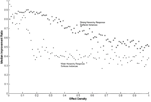
Weak Hierarchy Respon seH R Surfaces Instances * * * #*' *~* * * * * * * 4&. * * IIIII I I I I 0.1 0.2 0.3 0.4 0.5 Effect Density 0.6 0.7 0.8 0.9 1
Figure 3.5: Median Improvement Ratio verses Effect Density for both Strong and Weak Hierarchy Response Surface Instances
3.2.5 Conclusions from Probability Model
The use of compound noise as robust design method leads to reduction in experimental effort. Up till now we have tried to gage the effectiveness of compound noise as a robust design method for response surface instances generated using Strong and Weak
E 0 E