HAL Id: hal-01924957
https://hal.archives-ouvertes.fr/hal-01924957
Submitted on 18 Feb 2020
HAL is a multi-disciplinary open access archive for the deposit and dissemination of sci-entific research documents, whether they are pub-lished or not. The documents may come from
L’archive ouverte pluridisciplinaire HAL, est destinée au dépôt et à la diffusion de documents scientifiques de niveau recherche, publiés ou non, émanant des établissements d’enseignement et de
Path instability on a sphere towed at constant speed
Martin Obligado, Nathanaël Machicoane, Agathe Chouippe, Romain Volk,
Markus Uhlmann, Mickaël Bourgoin
To cite this version:
Martin Obligado, Nathanaël Machicoane, Agathe Chouippe, Romain Volk, Markus Uhlmann, et al.. Path instability on a sphere towed at constant speed. Journal of Fluids and Structures, Elsevier, 2015, 58, pp.99 - 108. �10.1016/j.jfluidstructs.2015.08.003�. �hal-01924957�
Path instability on a sphere towed at constant speed
Mart´ın Obligado1
Turbulence, Mixing and Flow Control Group, Department of Aeronautics, Imperial College London, London SW7 2AZ, United Kingdom
Nathana¨el Machicoane1
Laboratoire FAST, CNRS, Universit´e Paris-Sud, 91405 Orsay, France
Agathe Chouippe
Institute for Hydromechanics, Karlsruhe Institute of Technology, 76131 Karlsruhe, Germany
Romain Volk
Laboratoire de Physique, ENS de Lyon, UMR CNRS 5672, Universit´e de Lyon, Lyon, France
Markus Uhlmann
Institute for Hydromechanics, Karlsruhe Institute of Technology, 76131 Karlsruhe, Germany
Micka¨el Bourgoin
Laboratoire des ´Ecoulements G´eophysiques et Industriels, CNRS/UJF/G-INP, UMR5519, Universit´e de Grenoble, BP53, 38041, Grenoble Cedex 09, France
Abstract
The dynamics of towed objects in a fluid environment is of interest for many practical situations. In this article we report results for wake instabilities of spheres towed in a water tank. Six particles of different diameter and/or density ratio have been investigated, towed at 5 different constant veloci-ties. The explored density ratios lay within Γ ∈ [1.06; 2.56], with particle Reynolds numbers Rep ∈ [100; 1200], corresponding to Galileo numbers in
the range Ga ∈ [1300; 8000]. We introduce a surrogate Galileo number Ga∗ that, by taking into account the towing force applied to the particle, allows a comparison with the case of free falling/ascending spheres. Using innovative 3D tracking techniques, the three-dimensional trajectory of each particle is reconstructed. The wake instability for the studied particles is found to be associated to a 3D helicoidal motion with an elliptical cross section in the plane perpendicular to the towing direction. The 3D oscillatory motion was found independent of the particle density ratio, with a threshold of the or-der of Recp ∼ 355 (or Ga∗c ∼ 245). This threshold is slightly larger than the one found for the free falling particles’ transition to 3D chaotic motions (Rec
p ∼ 310 or Gac∼ 225).
Keywords: Towed spheres, wake instabilities, 3D tracking.
1. Introduction
The dynamics of towed objects in a fluid environment is of interest for many practical situations. In the context of these applications, it is often of crucial importance to warrant the stability of the trajectory of the towed object (at the tip of the cable), which turns out to be an interesting and
5
complex fluid dynamics problem. This work studies path instabilities of solid spheres towed at constant speed. The results obtained from this towed case are compared with the well studied problem of wake instabilities of free falling/ascending spheres.
The physical causes for the path instability of an arbitrarily shaped body
10
submerged in a viscous fluid can be separated in two classes. The first class, that applies only to non-spherical bodies, is related to the way the hydrody-namical forces and torques evolve when a disturbance is applied to the body degrees of freedom. The second class involves the wake instability that oc-curs beyond a critical Reynolds number even if the body is translating with
15
constant speed and orientation. Wake instabilities of the later kind have already been reported by Newton [1] when studying the drag of spheres in falling liquids. Over the last 15 years, with the advent of direct numerical simulation (DNS) at higher Reynolds number and high speed imaging tech-niques, this problem has received renewed attention [2, 3, 4, 5, 6, 7]. A big
20
variety of motions have been reported for such a system, a review on this subject can be found in [8] and a detailed historical review in [4].
Three basic parameters can be considered for studying free falling/ascending spheres. The first one is the particle Reynolds number Rep (defined as Rep = ΦUs/ν, where Us is the relative velocity between the fluid and the
25
sphere, Φ its diameter and ν the kinematic viscosity of the flow). The second one is the density ratio Γ = ρp/ρ0, where ρp and ρ0 are the particle and fluid densities respectively. And the third one is the Galileo number, defined as Ga =
q gΦ3ρ
0(ρp−ρ0)
µ2 , where g is gravity acceleration modulus and µ the fluid
dynamic viscosity. Dimensional analysis shows that the system is governed
30
by only two parameters. In this work, we will consider two different sets of parameters to study the stability of the spheres: Rep and Γ according to [8], and Ga and Γ as proposed by [5]. It is important to remark that the defi-nition of Ga for a towed case has to be adapted considering the differences between the towed and the free falling/ascending particle problem (see the
35
discussion about the definition of Ga in section 2).
The instabilities and thresholds for freely settling/rising spheres are sum-marized in a schematic regime map (Ga, Γ) in figure 1 and are detailed below. Wake instabilities are caused by two subsequent bifurcations, where the first occurs around a sphere at Ga1
c = 155 (or Re1pc = 212). The second,
40
which depends on the given value of Γ, is a Hopf bifurcation. In average, this bifurcation has critical values Ga2
c = 185 and Re2pc = 257 very close to those of the first bifurcation. For Reynolds numbers below the first bifur-cation, steady vertical motion with full axisymmetry in the horizontal plane is obtained. This bifurcation leads to a stationary state that is no longer
45
axisymmetric, yielding a regime with steady oblique motion. The second bifurcation is related to a periodic state, and the magnitude of the lift force associated with this mode oscillates around a mean value that can be differ-ent from zero. The resulting regime is therefore made of oscillating oblique paths, with low-frequency oscillations for 1 < Γ < 2.5 and high-frequency
50
oscillations for higher values of Γ. Spheres in this range of Ga, with a den-sity ratio lower than unity (i.e. ascending spheres), are reported to be in a ‘zig-zagging’ state (planar periodic oscillations). Transition to chaos occurs around Ga3c ∼ 225 or Re3
pc ∼ 310, when the wake of the sphere becomes fully three-dimensional, leading to many different regimes with important
quali-55
tative differences. Generally speaking, states with high Ga and low density ratio (close to the ‘zig-zagging’ regime) are highly intermittent, while for larger density ratios much less ordered states are observed.
Steady vertical path Planar -oblique oscilla ting pa th Planar -oblique st eady pa th Chaotic motions 100 150 200 250 1 3 5 7 9 Ga= gΦ3ρ0(ρp−ρ0) µ2 Γ = ρp ρ0
Figure 1: Schematic regimes map in the (Ga, Γ) parameter plane for the free falling/ascending spheres (image based on the results from [5, 7], simplified for Γ < 1). The left regime consists in steady vertical motions, that transit towards steady oblique trajectories confined in a plane after the solid line. The discontinuous dotted line is the second transition (Hopf bifurcation) that yields planar-oblique oscillating paths, while the continuous dotted line leads to a variety of chaotic motions.
that is orders of magnitude lower than its settling velocity. It is therefore an
60
intermediate case between the fixed sphere and the free falling/ascending case and it remains unclear whether results of free case can be applied. While in the free falling/ascending case the settling velocity is indirectly controlled by Γ and Ga, in our case this velocity can be prescribed independently. This is a new scenario in which these two parameters can be combined in new ways,
65
never explored systematically before. Nevertheless, as has been pointed out in [8] for the case of a sphere, the wake instability is the only candidate to generate oscillations. Therefore, some analogue instabilities should appear in the towed case. Yet, it is not evident how the tension of the towing cable would affect this motion.
70
The purpose of this work is to study such a towed system and to try to identify the critical values of Repc, Γcand Gac. Any differences with the free falling/ascending situation would be essential for the cited applications. We therefore investigate the stability of the trajectory of different classes of par-ticles, with various density ratios and Reynolds numbers. The experimental
75
characteris-tics are described in section 2. We evidence that trajectories can be unstable under certain conditions, the instability yielding to 3D oscillations (section 3). We characterize the destabilization of this system as a function of the particle’s Reynolds number in section 4. In section 5 we discuss the observed
80
instability in regards to wake instabilities of free falling spheres. We finally summarize the main results of this work in section 6.
2. Experimental setup
2.1. Towing system and tracking
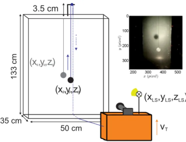
The experiment has been performed in a water tank (figure 2), with a
85
rectangular cross-section of dimensions 50 × 35 cm2 (in the x0z plane) and a height of 133 cm (along the y coordinate). More detailed information about the experimental setup can be found in [9, 10]. A platform that moves vertically along a rail is located in front of the tank, facing the particle. As can be appreciated in figure 2, the towing cable is arranged in such a
90
way that the particle and the platform displacement are exactly the same, setting the platform in the particle reference frame. The length of the cable between the highest position and the initial position of the particle (the part of the cable that affects the motion of the sphere) is of 1.1 m, with 3.5 cm of the cable out of the water (see next section for details of the cable). The
95
starting and ending positions are well away from the upper and lower tank boundaries to avoid any perturbation, yielding a total displacement of 75 cm and a wire length of 35 cm at the end of the experiment. A light source and a camera are fixed to the platform. This allows us to record the particle at a fixed height for all displacements, making it possible to record much longer
100
trajectories compared with the free falling case (of the order of 1 min). Five different towing velocities vT in the range 1 < vT < 3 cm/s with increments of 0.5 cm/s have been investigated for each class of sphere (see below). The use of the translation stage assures a constant towing velocity throughout the motion.
105
A white panel is placed on the back of the tank, in order to be able to track both particle and particle’s shadow. In section 3.2 we will show that this setup allows us to perform three-dimensional tracking of the spheres with only one camera.
Particle’s trajectories are recorded using a camera with a resolution of
110
640 × 380 pixels and an acquisition frequency of 30 Hz. Considering the towing speed and the dimensions of the tank, at least 25 s of trajectory were
Figure 2: Scheme of the experimental setup. The dashed line shows the wire (solid line) behind the tank. The light colours depict the particle’s and wire’s shadow and the arrows show the towing direction. The subscripts S, P and LS stand for shadow, particle and light source, respectively. The inset is a raw image taken with the camera, where one can clearly observe the particle and its shadow.
recorded, resulting in over 700 frames. In order to have statistical conver-gence for each class of sphere, 10 movies are recorded for each sample. The conversion from pixels to length units is made using known printed patrons
115
(masks) which allows us to determine the projective transformation between pixels and real world units. Two different masks are used: one at the back of the tank to convert the positions of the particle shadow and another in the plane x0y (where the origin of coordinates is placed at the initial po-sition of the sphere) for the particle’s popo-sitions. Then, both the particle’s
120
and its shadow trajectories are obtained using standard 2D tracking tech-niques. Section 3.2 explains how the combined tracking of the particle and its shadow yield the particle 3D trajectory. As the particle can experience a three-dimensional motion, an approximation is needed. This approximation consists in applying the same 2D transformation to the particle, regardless
125
of its z position. This is only valid if the displacement ∆z of the particle is small compared to the distance between the sphere and the camera D. As it will be shown in section 3.2, the particle displacement in z coordinate is around a few millimetres at most, while the camera is at 50 cm from the sphere, so we effectively verify ∆z/D 1.
130
through a slight vibration of the system. To recover the underlying smooth signal, we use a filtering method based on cubic spline interpolations. Note that in our case the filtering is quite straightforward and non-ambiguous, considering the much higher frequency of the vibrations (above 10Hz)
com-135
pared to the main oscillations of the spheres (a fraction of Hertz). In this way, we are able to filter most of the noise without affecting the actual signal. 2.2. Particles
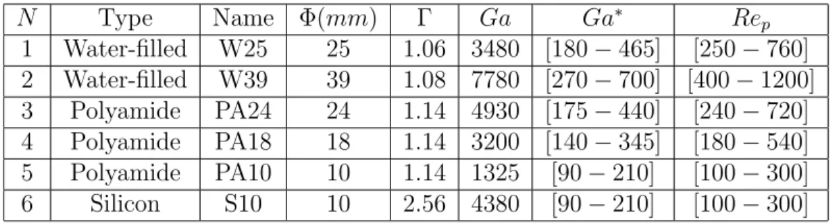
Six different types of particles are analyzed, exploring a wide range of Ga, Rep (defined as Rep = vTΦ/ν with vT the towing velocity) and Γ. The
140
wire used to tow the spheres is a simple cotton fiber, with a diameter of the order of 100 µm, negligible stiffness and a linear density of less than 30 mg/m. The wire density and mass are orders of magnitude lower than the spheres. It has been checked that the wire alone does not exhibit any instabilities (i.e. oscillations or transverse displacements). The properties
145
of the particles can be found in table 1. The column labeled Ga∗ shows a surrogate Galileo number based on the wire tension, defined to adapt this parameter to a towed situation instead of a free falling one. We consider that in the most general case the Galileo number can be written as Ga = pF Φ3/mp/ν, mp being particle’s mass and F the “traction” force; therefore
150
the Archimedes force, g(mp−m0), with m0 the mass of displaced fluid for the free falling case. In our situation the Archimedes force has to be replaced by the wire’s tension. In a stable towing situation, the wire’s tension is exactly balanced by the drag force on the sphere: Tz = FD = 12ρ0π(Φ/2)2vT2CD, obtaining Ga∗ = pFDΦ3/mp/ν = Repp3CD/4. The drag coefficient for
155
static spherical particles is well tabulated (see for instance [3, 11]), so we have used the commonly accepted values according to the particle Reynolds number of our particles. It is important to remark that for the values of Rep studied, CD may have a strong dependency with Rep. Therefore, although Ga∗ is absolutely defined by Rep, each characteristic number can give a
160
different trend when comparing with other parameters.
3. Evidence of an instability 3.1. Particle trajectories
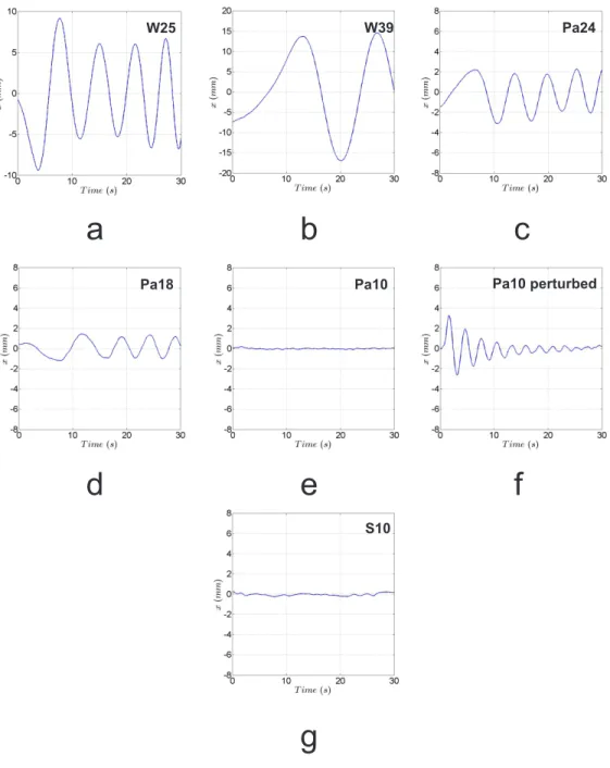
The main objective of this experiment is to study possible instabilities of a sphere submerged in water and towed at constant speed. Figure 3
165
N Type Name Φ(mm) Γ Ga Ga∗ Rep 1 Water-filled W25 25 1.06 3480 [180 − 465] [250 − 760] 2 Water-filled W39 39 1.08 7780 [270 − 700] [400 − 1200] 3 Polyamide PA24 24 1.14 4930 [175 − 440] [240 − 720] 4 Polyamide PA18 18 1.14 3200 [140 − 345] [180 − 540] 5 Polyamide PA10 10 1.14 1325 [90 − 210] [100 − 300] 6 Silicon S10 10 2.56 4380 [90 − 210] [100 − 300]
Table 1: Characteristics of the particles considered. The density ratio Γ is calculated considering that ρ0= 997 kg/m3 for water at 25◦C.
vT = 2 cm/s, in a one-dimensional representation of one transverse com-ponent for a better visualization of the instabilities. This qualitative visual inspection of the trajectories is sufficient to evidence the existence of an in-stability for towed sphere. For instance, particle PA10 clearly appears as
170
stable (figure 3e). This is further confirmed when the particle is initially per-turbed: the rapid oscillations imposed are damped quickly (figure 3f). This proves that possible small variations of the wire length (due for instance to small elongation of the cotton cable) do not bias the instability diagnosis by excitation of possible instabilities. Particle PA24 on the contrary is a clear
175
case of instability (figure 3c), where without any external perturbation, an oscillating motion grows spontaneously.
The oscillations observed for unstable towed spheres are qualitatively sim-ilar to those evidenced for the free falling sphere. However, in the later case, the motion can take place in a plane or in the 3D space. Is the present
180
instability of the zig-zag (2D) type or is it three-dimensional? In the next subsection, we address this question, gaining access to the 3D particle trajec-tories by tracking not only each particle position, but the one of its shadow. 3.2. 3D trajectories
In this section we introduce a reconstruction of the 3D trajectory of the
185
towed sphere with this simple one-camera setup, that only demands to ac-curately measure the position of the particle, the one of its shadow and that of the light source. With only one camera and a light source, but under certain conditions, the shadow projected by an object on a wall can be used to measure its out-of-plane coordinate. In [12] such an approach is used to
190
a
b
c
d
e
f
g
W39 Pa24
Pa18 Pa10 Pa10 perturbed
S10 W25
Figure 3: Trajectories obtained for all the particles shown in table 1. For particle PA10 we also show the trajectory of the particle after being initially perturbed in order to study the robustness of the stability.
a new approach allowing to reconstruct the full 3D trajectories of particles motion in the bulk of the flow.
Particle and shadow trajectories are easily obtained via standard tracking techniques while light source position has been obtained indirectly, assuming
195
a virtual point-like source approximation. The light source is virtual because of the refraction effects of the air-PMMA-water interfaces at the sides of tank’s walls. Therefore the point source approximation will only be valid if the angles explored by the particle (with respect to particle’s initial position) are small enough. In a first step the position of the virtual light source
200
is obtained. As schemed in figure 2, we denote the light source position (xLS, yLS, zLS), the particle’s (xP, yP, zP) and its shadow’s (xS, yS, zS). As these three points are aligned, they follow the parametric equation:
xP yP zP = xS yS zS + p xLS − xS yLS − yS zLS − zS (1)
Provided that the only measured coordinates are xP, yP, xS, yS and zS (the shadow is projected onto a plane at constant z), it is necessary to add more
205
equations to solve the system. For that purpose, it is enough to consider the positions in the instant t = 0 s, when the sphere is still static and placed in its initial position:
xLS yLS zLS = x0 S y0 S zS0 + p1 x0 P − x0S y0 P − y0S zP0 − z0 S (2)
where now the three components of the initial position of the particle and its shadow are known. This system is finally composed by six equations and six
210
unknowns (zP,p,p1,xLS,yLS and zLS) and should have a unique solution. Yet these three points are aligned in physical space, but the points obtained by tracking, even assuming sub-pixel accuracy, are not exactly aligned (taking into account measurement errors). As the system of equations to solve is complex and has many variables, this results in a very noisy estimation of
215
the z component of the particle.
In order to solve this problem we proceed iteratively. In a first iteration, we focus on deducing only the position of the light source (xLS, yLS, zLS). This is made by solving the full problem at each time step and obtaining a robust estimate of the light source position as the time average of this first
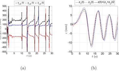
(a) (b)
Figure 4: (a) Light source position obtained solving equation systems (1) and (2). (b) z coordinate of the particle solving equation system (1) (blue and red). Black dashed line represents the mean value of previous curves. The curves on figures (a) and (b) correspond to the particle PA24 towed at 2 cm/s
solution. Figure 4(a) shows the position of the light source obtained for each time step for a typical unstable case. It can be appreciated that a clear mean value emerges from the noise. This value will be considered as the position of the point-like virtual light source. The diverging deviations from this mean value occur when the particle returns to its initial position and ~xp ∼ ~x0p.
225
In this situation, the system composed by equations (1) and (2) becomes under-constrained. With the light source position and the amplitudes shown in figure 3, we verify that the angles explored by the particles are lower than 1o. This is a small enough angle to neglect legitimately the departure from a point-like source approximation due to refraction in the interfaces.
230
Nevertheless, the approximation of the finite lamp by a point-like source is needed.
Once the lamp position is known, the system can be decomposed in two linear systems with two equations each, the first only considering x and z coordinates and the other considering y and z coordinates. Hence, two
235
solutions for the z component of the particle are obtained as shown in figure 4(b). This allows us to verify the consistency of the system, as both solutions
are similar. It also allow us to finally define the z component of the particle as the average of both solutions, improving the accuracy.
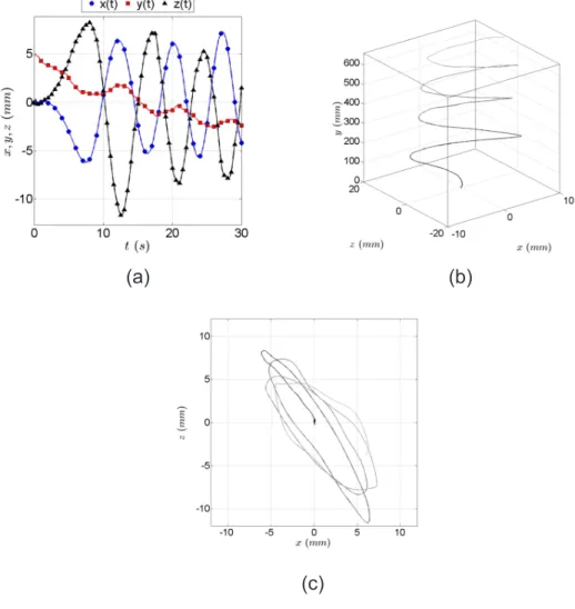
Figure 5(a) shows the three components of the position of the particle
240
in time domain (in the towed frame), while figure 5(b) shows the resulting particle trajectory in the real space presenting an elliptical spiraling path. The projected trajectory in the x0z plane (figure 5(c)) is in fact an ellipse. The eccentricity of the ellipse tends to decrease with time: the initial motion is almost planar, and then becomes ellipsoidal, with a trend towards a circular
245
motion if the tank would have been longer. Consistently, the phase shift in figure 5(a) between x and y coordinates exhibits a trend towards quadrature (signature of a circular motion) as time evolves. This may be interpreted as a possible signature of a transition from 2D zig-zagging to 3D spiral paths, or an effect linked to the decreasing length of the cable. Further experiments
250
in a taller tank would be required to be conclusive on the eventual terminal circularity of the motion in x0z plane and the possible influence of the finite length of the cable.
On figure 5(a), one can observe a small change of the vertical coordinate y in the moving frame (about 7 mm to be compared to the total vertical
255
displacement ymax = 750 mm in the reference frame). As the towing cable is made of cotton fiber, it suffers a small elongation during the trajectory caused by its elasticity, which produces small variations in the vertical component of the trajectory. As emphasized before, the stable case quickly damps any perturbation, and the local variations of the fiber length are very small
com-260
pared to the magnitude of the oscillation, so we can consider them negligible and non affecting the instability diagnosis.
As a partial conclusion, this analysis shows that the trajectory of towed particles can become unstable, being subject to 3D oscillations. What trig-gers the onset and controls the amplitude of these oscillations will be
dis-265
cussed in section 4.
To finish this section, it is important to emphasize the simplicity of this 3D tracking method. It is only necessary to assume a small displacement of the tracked particle (compared to the distance to the camera and the light source) and a point-like light source. It is always possible to add more
270
cameras, that will expand the number of linear equations allowing us to better determine, in a first step, the position of the light source. In a second step, each camera will provide two different solutions for 3D particle position (as in figure 4b), giving more solutions to average and increase the tracking precision. In other words, the proposed method can be used in conjunction
(a) (b)
(c)
Figure 5: (a) Three Cartesian components of the particle in the moving frame as a function of time (with only a few symbols for visibility). The apparent important variation of y, due to the wire elasticity, is in fact dwarfed by the maximum real altitude ymax= 750 mm. Three dimensional trajectory of the particle in the laboratory frame (b) and its projection in the x0z plane (c); the black to gray colormap represents the time evolution.
with usual multi-cameras stereo matching methods, where the additional information from the shadow images gives further redundancy improving the accuracy of the particle’s 3D positioning. An alternative would be to add more light sources obtaining new shadows to track.
4. Instability characterization
280
The simple observations of the particle trajectories (figure 3) lead us to think that increasing the particle size can trigger this oscillating instability, but no clear critical diameter can be deduced, as this transition also depends on the towing speed. For a more quantitative analysis on the influence of vT, φ and Γ, we propose to investigate the onset of instability from the particle’s
285
velocity as a signature of the existence of transverse motion. We base our analysis on averaged trajectories and focus here on the threshold and the am-plitude of the instability. In the previous section, we found that the projected trajectories in the x0z plane are elliptical. As the direction of each ellipse semi-axis is random in space for each measurement, the trajectory averaged
290
over a large number of measurements will converge to a circle. Therefore, the rms velocity of the one-dimensional trajectories x(t) represents, after av-eraging over 10 trajectories, the averaged velocity component in the polar direction in the x0z plane. The velocity amplitude vθ obtained is then the characteristic velocity of the whole trajectories and describes not only the
295
presence but also the magnitude of the instability. For the case of a stable trajectory (hence almost linear), we have checked that the rms value is equal to the measurement noise (which we estimate of the order of 10−4m/s), while for oscillating cases, this value is linked to the amplitude and frequency of the oscillation. Therefore, before we estimate the average velocity vθ for each
300
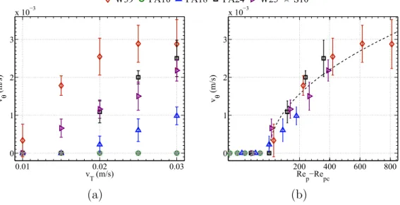
of the investigated configurations, we arbitrarily set to 0 any velocity events lower than the measurement error coming from the particle center detection. Figure 6(a) shows the velocity vθ, as a function of the towing speed for the different particles tested, without any normalization. One can observe differ-ent trends for the set of particle parameters and towing speed investigated:
305
some trajectories are always unstable or always stable independently of vT, while the trajectory of some particles become unstable when increasing vT. The corresponding critical towing speed seems therefore to depend on the particle characteristics.
As explained in the introduction, one of the natural relevant parameters
310
0.01 0.02 0.03 0 1 2 3 x 10⁻³ vT (m/s) vθ (m/s) 200 400 600 800 0 1 2 3 x 10⁻³ Rep−Repc v θ (m/s) −200 0 200 400 600 800 0 0.05 0.1 0.15 0.2 0.25 vθ / (vT 3 CD / 4)
W39 PA10 PA18 PA24 W25 S10 Uhlmann and Dusek
(a) (b)
Figure 6: a) Polar rms velocity vθ of the particle as a function of the towing speed vT for all cases considered. b) Polar rms velocity vθ of the particle as a function of particle Reynolds number Repfor all cases considered. The black dashed line is a fit according to vθ= ApRep− Repc.
particle diameter, but ignoring its density ratio, we find that this Reynolds number is the good parameter for this instability, as can be observed on figure 6(b): the polar velocity is null for small Reynolds number, then starts to increase after a critical value (Rec
p ∼ 355), and seems to saturate for the
315
highest Reynolds numbers.
The instabilities seem to follow a universal law for vθ, independent of Γ, close to the simple relation vθ = ApRep− Repc, with Repc = 355 and A = 0.1 mm/s a constant velocity amplitude. It is remarkable to note that vθ scaling withpRep− Repc is compatible with a classical super-critical
in-320
stability and a cubic non-linear saturation mechanism [13], associated to the invariance in vθ = −vθ transformation (the direction in which the sphere describes the elliptical spiral motion is not prescribed). In this context, the instability may be modelled by a classical symmetry preserving instability equation: dvθ/dt = α(Rep− Repc)vθ+ βvθ3. The cubic term reflects the
non-325
linear saturation mechanisms of the instability, for which we do not have any particular physical insight at the moment.
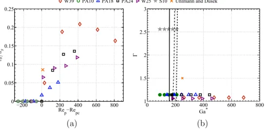
−200 0 200 400 600 800 0 0.05 0.1 0.15 0.2 0.25 Rep−Repc vθ /u ∗ g 0 200 400 600 800 1 1.5 2 2.5 3 Ga* Γ −200 0 200 400 600 800 0 0.05 0.1 0.15 0.2 0.25 Re−Rec vθ / (vT 3 CD / 4)
W39 PA10 PA18 PA24 W25 S10 Uhlmann and Dusek
(a) (b)
Figure 7: (a) Normalized polar velocity vθ/vg∗for all the studied particles as a function of Rep− Repc. (b) Diagram of instabilities in the (Ga∗, Γ) parameter plane for the towed particles in this experiment with the adapted parameter Ga∗. The filled symbols stand for stable regimes and the empty ones for unstable cases. The lines represent the threshold for different instabilities for free falling/ascending spheres. The solid line shows the threshold of the first instability and the discontinuous and continuous dashed lines represent the Hopf bifurcation (at lower Ga) and the transition to chaos (at higher Ga) respectively. For both figures, the orange cross is a numerical point obtained in [7] for a free-falling sphere with a classical Galileo number Ga = 250 and Γ = 1.5.
the raw (non normalized) velocity vθ itself.
The good collapse observed using only Rep tends to confirm that a proper
330
Galileo number in a towed system would be Ga∗ = Repp3CD(Rep)/4 (as CD is a function only of Rep, Ga∗ will also be only a function of Rep). We consequently introduce a surrogate vertical velocity u∗g, derived from Ga∗ ac-cording to Ga∗ = u∗gΦ/ν, yielding u∗g = vTp3CD/4. With this normalization (figure 7(a)) the experimental points are more scattered than in figure 6(b),
335
but a numerical datum from [7], corresponding to a free falling sphere in the chaotic regime, is located very close to the experimental data.
Finally, figure 7(b) shows the regimes map in the (Ga∗, Γ) parame-ter plane obtained with the results from this experiment, with the free falling/ascending regimes delimited by the numerical studies of [5, 7]. This
340
diagram shows that the instability threshold observed here for the case of towed spheres coincides very closely to that of the transition towards the full 3D chaotic regime for free falling/ascending spheres (Ga ∼ 225). We can
thus conclude that towed particles have a three-dimensional helicoidal regime consistent with the transition to chaos for free falling/ascending particles.
345
5. Discussion
In this article we studied spheres towed at constant velocity varying their density ratio Γ, their diameter Φ and the towing speed vT. The threshold for the 3D oscillatory motion was found of the order of Repc ∼ 355 (or Ga∗c ∼ 245). This is slightly larger than the threshold found for the free
350
falling particles’ transition to 3D chaotic motions. On the other hand, as can be seen in figure 1, if the usual definition of Ga based on the settling velocity is used (see table 1), all particles are well into the chaotic regimes and no stable cases would be expected. Therefore, the definition of the surrogate Galileo number Ga∗ is appropriate in order to compare the free falling/ascending
355
and the towing cases. Nevertheless, the difference in thresholds shows that the cable is playing an important role in the dynamics of towed spheres.
It is not clear whether this case can be totally related to the free falling/ascending case. The main difference between both cases is that the velocity (the
tow-ing velocity in our case, the settltow-ing velocity for the free falltow-ing case) does
360
not depend on Γ for the towed system. Evidence of this is that the onset of the instabilities for the particles explored can be characterized with only one parameter (Ga∗ or equivalently Rep) while for the free falling/ascending case the density ratio has to be considered. Although the thresholds for in-stability are similar in both cases, only the case of towed spheres presents a
365
three-dimensional helicoidal instability. This is an important difference with free falling/ascending spheres, where many different regimes exist, but not this one in particular. This regime is observed only in free falling/ascending cylinders [14] and bubbles with oblate spheroidal shapes [15]. This may be caused by the influence of the towing cable in the dynamics, affecting the
370
wake of the sphere or generating a coupling of the unstable motion with a pendular one via a restoring force.
We note that [16] finds that for Rep ∼ 355 a fixed sphere experiences tran-sition to chaos. The similarity between the three thresholds (free falling/ascending, towed and static spheres) certifies the hypothesis that the instabilities
ob-375
served in this work are linked to the wake transition behind an object (whether fixed or not).
Despite the clear influence of the cable in the motion of the particle, no other reminiscences of a pendulum have been found. It is important
to remark that the observed frequencies should be time dependent as the
380
length of the cable decreases and the particle travels upwards. The frequency of such pendulum has been computed and was shown to be different from those observed for towed spheres but still in the same order of magnitude. It has also been checked that the observed frequencies are not consistent with those expected from vortex shedding, which present a typical Strouhal
385
number of 0.2. The measured frequencies would give a Strouhal number of approximately 0.6. Then, these instabilities are very likely related to similar physical causes than wake instabilities observed for free falling/ascending spheres. Comparing with the free falling/ascending diagram, the trigger of the instability for towed spheres seems to be related to the transition
390
towards the chaotic, fully three-dimensional wake. It also seems related to a super-critical instability with a cubic non-linear saturation mechanism. The exact mechanisms for this saturation is less clear: if we consider the elliptical motion of the sphere in the horizontal plane, a saturation of vθ may imply a balance between the centripetal acceleration, the tension of the cable and
395
a lift force that the instability develops. Although the tension of the cable and therefore the centripetal acceleration may be modeled using the mean drag force on the sphere, it is not possible to model the lift force based on our experimental setup. This lack of information becomes evident in figures 6(b) and 7(a). While the raw value of vθ gives a very good collapse, the
400
normalized velocity vθ/vg∗ gives a worse one but allows to collapse numerical data from free falling particles. This absence of a proper normalization shows that even for the simplified system of a towed sphere we are far from having a full understanding of the wake instability phenomenon. The lift force arising from the instability and the contribution of the component of drag force in
405
the x0z plane may play a role in the normalization of vθ. Furthermore, non-trivial effects, as another onset for instabilities caused by the sphere acting as a stochastic harmonic oscillator (as studied in [17]), with the forcing of the three-dimensional wake in the chaotic regime may be considered. Numerical studies would be then of great importance in order to shed some light on the
410
instabilities of towed spheres.
6. Summary
We conclude this article with a summary of the main points of our work. In this study we have analyzed the wake instabilities of a towed sphere in a
laminar flow. The main results can be summarized as:
• A very broad set of experimental points in the parameter space [Γ, Rep, Ga∗] has been explored. In total, 30 different cases have been col-lected, with density ratios ranging from 1.06 to 2.56, surrogate Galileo num-bers Ga∗ from 90 to 700 and particle Reynolds numbers from 100 to 1200.
420
• An innovative experimental technique is proposed, based in a towing system, that allowed us to control independently Γ and Rep. This is a signifi-cant advantage compared to the free falling/ascending situations where both parameters are coupled via the terminal velocity. Nevertheless, the introduc-tion of a surrogate Galileo number still allows for comparison of both cases.
425
A simple but effective three dimensional tracking tool has been developed that only requires one generic camera and the image of the particle and its shadow. It has allowed us to characterize the instabilities present for towed spheres as 3D helicoidal paths with an elliptical cross section in the plane perpendicular to the towing direction.
430
• A threshold for oscillatory motion has been identified of Repc ∼ 355 (or Ga∗c ∼ 245). Unlike the case of the free falling/ascending sphere, this threshold is found to be independent of Γ.
Acknowledgements
The authors want to thank Jan Duˇsek for stimulating discussions and
435
Dieter Groß, J¨urgen Ulrich and Michael Ziegler for experimental support. This work was supported by the Franco-German research program PRO-COPE (grants 26803QD and 54366584) and the German Research Founda-tion (DFG) under project UH 242/1-2.
440
References References
[1] I. Newton, The principia: mathematical principles of natural philosophy, Univ of California Press, 1999.
[2] C. Veldhuis, A. Biesheuvel, D. Lohse, Freely rising light solid spheres,
445
International Journal of Multiphase Flow 35 (4) (2009) 312–322.
[3] R. Clift, J. R. Grace, M. E. Weber, Bubbles, drops, and particles, Courier Dover Publications, 2005.
[4] M. Horowitz, C. Williamson, The effect of reynolds number on the dy-namics and wakes of freely rising and falling spheres, Journal of Fluid
450
Mechanics 651 (2010) 251.
[5] M. Jenny, J. Duˇsek, G. Bouchet, Instabilities and transition of a sphere falling or ascending freely in a newtonian fluid, Journal of Fluid Me-chanics 508 (1) (2004) 201–239.
[6] T. Deloze, Y. Hoarau, J. Duˇsek, Transition scenario of a sphere freely
455
falling in a vertical tube, Journal of Fluid Mechanics 711 (2012) 40. [7] M. Uhlmann, J. Duˇsek, The motion of a single heavy sphere in ambient
fluid: a benchmark for interface-resolved particulate flow simulations with significant relative velocities, International Journal of Multiphase Flow 59 (2014) 221–243.
460
[8] P. Ern, F. Risso, D. Fabre, J. Magnaudet, Wake-induced oscillatory paths of bodies freely rising or falling in fluids, Annual Review of Fluid Mechanics 44 (2012) 97–121.
[9] G. K¨uhn, DorktorArbeit: Untersuchungen zur Feinsedimentdynamik unter Turbulenzeinfluss, Univ.-Verlag Karlsruhe, 2007.
465
[10] B. Westrich, U. F¨orstner, Sediment dynamics and pollutant mobility in rivers (sedymo): assessing catchment-wide emission-immission relation-ships from sediment studies. bmbf coordinated research project sedymo (2002–2006), Journal of Soils and Sediments 5 (4) (2005) 197–200. [11] P. P. Brown, D. F. Lawler, Sphere drag and settling velocity revisited,
470
Journal of Environmental Engineering 129 (3) (2003) 222–231.
[12] G. A. Voth, A. la Porta, A. M. Crawford, J. Alexander, E. Boden-schatz, Measurement of particle accelerations in fully developed turbu-lence, Journal of Fluid Mechanics 469 (1) (2002) 121–160.
[13] E. L. LD Landau, Course of Theoretical Physics, vol 6: Fluid mechanics.,
475
Butterworth-Heinemann, 1987.
[14] P. C. Fernandes, F. Risso, P. Ern, J. Magnaudet, Oscillatory motion and wake instability of freely rising axisymmetric bodies, Journal of Fluid Mechanics 573 (2007) 479–502.
[15] G. Mougin, J. Magnaudet, Path instability of a rising bubble, Physical
480
review letters 88 (1) (2001) 014502.
[16] R. Mittal, Planar symmetry in the unsteady wake of a sphere, AIAA journal 37 (3) (1999) 388–390.
[17] R. Bourret, U. Frisch, A. Pouquet, Brownian motion of harmonic oscil-lator with stochastic frequency, Physica 65 (2) (1973) 303–320.
![Figure 1: Schematic regimes map in the (Ga, Γ) parameter plane for the free falling/ascending spheres (image based on the results from [5, 7], simplified for Γ < 1).](https://thumb-eu.123doks.com/thumbv2/123doknet/14402455.510219/5.918.306.616.189.454/figure-schematic-regimes-parameter-falling-ascending-spheres-simplified.webp)