Communication complexity of permutation-invariant functions

(1)

Communication Complexity of

=

Permutation-Invariant Functions

<

LL Go

by

o

PRITISH KAMATH

B.Tech. (Honors), Computer Science & Engg, IIT Bombay (2012)

Submitted to Department of Electrical Engineering and Computer Science

in partial fulfillment of the requirements for the degree of

Master of Science in Computer Science & Engineering

at

MASSACHUSETTS INSTITUTE OF TECHNOLOGY JUNE 2015

Massachusetts Institute of Technology 2015. All rights reserved.

AUTHOR:

Signature

Dept. of Electrical

CERTIFIED BY.

redacted

Engineering and Computer Science

May 20, 2015

Signature redacted

Madhu Sudan

Adjunct Professor of Computer Science and Engineering

Thesis Supervisor

ACCEPTED BY.

Signature redacted

Leslie A.k&Udziejski

Professor of Electrical Engineering

Chairman, Department Committee for Graduate Students

(2)

(3)

Communication Complexity of Permutation-Invariant Functions

by

PRITISH KAMATH

Submitted to Department of Electrical Engineering and Computer Science on May 20, 2015, in partial fulfillment of the requirements for the degree of

Master of Science in Computer Science & Engineering

Abstract

Motivated by the quest for a broader understanding of communication complexity of sim-ple functions, we introduce the class of "permutation-invariant" functions. A partial function

f

: {0, 1}" x {0, 1}" -. {0, 1, ?} is permutation-invariant if for every bijection : {1,..., n} -+

{1,.. ., n} and every x, Y E {0, I}", it is the case that f (x, y) = f (x', y'). Most of the commonly studied functions in communication complexity are permutation-invariant. For such functions, we present a simple complexity measure (computable in time polynomial in n given an implicit description of

f)

that describes their communication complexity up to polynomial factors and up to an additive error that is logarithmic in the input size. This gives a coarse taxonomy of the communication complexity of simple functions. Our work highlights the role of the

well-known lower bounds of functions such as SET-DISJOINTNESS and INDEXING, while com-plementing them with the relatively lesser-known upper bounds for GAP-INNER-PRODUCT (from

the sketching literature) and SPARSE-GAP-INNER-PRODUCT (from the recent work of Canonne

et al. [ITCS 2015]). We also present consequences to the study of communication complexity with imperfectly shared randomness where we show that for total permutation-invariant func-tions, imperfectly shared randomness results in only a polynomial blow-up in communication complexity after an additive O(log log n) loss.

Thesis supervisor: Madhu Sudan

(4)

(5)

Acknowledgments

I am very fortunate and grateful to have Madhu Sudan as my advisor, something which I could not have conceived when I first met him in Microsoft Research India, in 2013! Madhu is a rare combination of a brilliant researcher, caring mentor and a humble, friendly personality. I am truly looking forward to working with and being advised by Madhu during the rest of my PhD. studies.

I also thank Badih Ghazi for fruitful collaborations that we have been involved in. Indeed this thesis is based on a work [GKS15] joint with Badih and Madhu. I am very inspired by Badih's confident yet soft-spoken approach to research.

Special thanks to Akamai for their fellowship and also to NSF for the grants CCF-1218547 and CCF-1420956 that I have been supported by.

I would like to thank Dana Moshkovitz from whom I have gained a lot of knowledge and perspective. Also, I specially thank Michael Forbes for all the general guidance and care he has shown me.

I am greatly indebted to my previous mentor, Neeraj Kayal and collaborators, Ankit Gupta and Ramprasad Saptharishi (at Microsoft Research India), who have helped me understand the importance of discipline and work ethic needed to produce good research; something that I am always striving towards achieving. I also thank my undergraduate mentors Supratik Chakraborty and Nutan Limaye for encouraging and inspiring me to take up graduate studies. It has been my greatest privilege to be part of the amazing Theory CS group at MIT. The sheer number of awesome professors, post-docs and students all around has given me so much perspective in life! I especially thank professors Scott Aaronson and Ronitt Rubinfeld and also Mohammad Bavarian, Matt Coudron, Alan Guo, Jerry Li, Gautam "G" Kamath, Robin Kothari, Prashant Vasudevan and Henry Yuen. I am very grateful to administrative assistants Joanne Hanley, Debbie Lehto, Linda Lynch, Patrice Macalusco, Rebecca Yadegar for making the Theory group as vibrant as it is.

Life at MIT wouldn't have been as much fun without great company outside of work. I would like to thank Yashovardhan Chati, Devendra Shelar, Rajan Udwani, Vaibhav Unhelkar among many others. I also thank all my undergraduate friends who have always been an integral part of my life.

Finally I would like to thank my family: my late father Uday, my mother Urmila ('Amma'), aunt Naina (Atee'), grandmother Mukta (Ammu') for their love and support. And most impor-tant of all my elder brother Sudeep, who has been a guiding light throughout my life, and my girlfriend Apoorvaa Deshpande, who has provided me with immense moral support. Together, Sudeep and Apoorvaa have shaped me into who I am, and time and again, have made me understand things about myself which I could not have otherwise.

(6)

(7)

Chapter 1 Introduction

Communication complexity, introduced by Yao [Yao79], has been a central object of study in complexity theory. In the two-way model, two players, Alice and Bob, are given private inputs x and y respectively, along with some shared randomness, and they exchange bits according to a predetermined protocol and produce an output. The protocol computes a function

f

(-, -) if the output equals

f

(x, y) with high probability over the randomness 1. The communication complexity of f is the minimum over all protocols computing

f

of the maximum, over inputs x and y, of the number of bits exchanged by the protocol. The one-way communication model is defined similarly except that all the communication is from Alice to Bob and the output is produced by Bob. For an overview of communication complexity, we refer the reader to the book [KN97] and the survey [LSO9].

While communication complexity of functions has been extensively studied, the focus typi-cally is on lower bounds. Lower bounds on communication complexity turn into lower bounds on Turing machine complexity, circuit depth, data structures, streaming complexity, just to name a few. On the other hand, communication complexity is a very natural notion to study on its own merits and indeed positive results in communication complexity can probably be very useful in their own rights, by suggesting efficient communication mechanisms and paradigms 'In this work, we also consider partial functions where f(x,y) may sometimes be undetermined, denoted f (x,y) = ?. In such cases, the protocol can output anything when f (x,y) is undetermined.

(10)

in specific settings. For this perspective to be successful, it would be good to have a compact pic-ture of the various communication protocols that are available, or even the ability to determine, given a function

f,

the best, or even a good, communication protocol for

f

. Of course such a goal is overly ambitious. For example, the seminal work of Karchmer and Wigderson [KiW90] implies that finding the best protocol for

f

is as hard as finding the best (shallowest) circuit for some related function

f

.

Given this general barrier, one way to make progress is to find a restrictive, but natural, subclass of all functions and to characterize the complexity of all functions within this class. Such approaches have been very successful in the context of non-deterministic computation by restricting to satisfiability problems [Sch78], in optimization and approximation by restricting to constraint satisfaction problems [Cre95, KSTWOO], in the study of decision tree complexity by restricting to graph properties [Ros73], or in the study of property testing by restricting to certain symmetric properties (see the survey [Sud10] and the references therein). In the above cases, the restrictions have led to characterizations (or conjectured characterizations) of the complexity of all functions in the restricted class. In this work, we attempt to bring in a similar element of unification to communication complexity.

In this work, we introduce the class of "permutation-invariant" (total or partial) functions.

Let [n] denote the set {1, - -- , n}. A function

f

: {0, 1} x {0, I}" -* {0, 1, ?} is permutation invariant if for every bijection 7 : [n] -- [n] and every x, y E {0, 1 }" it is the case that

f

(x, y)=

f

(x,y'). We propose to study the communication complexity of this class of functions. To motivate this class, we note that most of the commonly studied functions in

communica-tion complexity including EQUALITY [Yao79], (GAP) HAMMING DISTANCE [Woo04, JKSO8, CR12, Vidi 1, She12, PEG86, Yao03, HSZZO6, BBG14], (GAP) INNER PRODUCT, (SMALL-SET)

DISJOINT-NESS [KS92, Raz92, HWO7, ST13], SMALL-SET INTERSECTION [BCK+14] are all

permutation-invariant functions. Other functions, such as INDEXING [JKS08], can be expressed without changing the input length significantly, as permutation-invariant functions. Permutation-invariant functions also include as subclasses, several classes of functions that have been well-studied

(11)

in communication complexity, such as (AND)-symmetric functions [BdWOl, Raz03, Shell] and XOR-symmetric functions [ZS09]. It is worth noting that permutation-invariant func-tions are completely expressive if one allows an exponential blow-up in input size, namely, for every function f(x,y) there are functions F, A, B s.t. F is permutation-invariant and f (x, y) = F(A(x), B(y)). So results on permutation-invariant functions that don't depend on

the input size apply to all functions. Finally, we point out that permutation-invariant func-tions have an important standpoint among funcfunc-tions with small communication complexity, as permutation-invariance often allows the use of hashing/bucketing based strategies, which would allow us to get rid of the dependence of the communication complexity on the input length n. We also note that functions on non-Boolean domains that are studied in the liter-ature on sketching such as distance estimation (given x,y E R", decide if lix - ylJ d or if lix - ylII > d(l + e)) are also permutation-invariant. In particular, the resulting

sketch-ing/communication protocols are relevant to (some functions in) our class.

1.1 Coarse characterization of Communication Complexity

Permutation-invariant functions on n-bits are naturally succinctly described (by 0(n3) bits).

Given this natural description, we introduce a simple combinatorial measure m(f) (which is easy to compute, in particular in time poly(n) given f ) which produces a coarse approximation of the communication complexity of f. We note that our objective is different from that of the standard objectives in the study of communication complexity lower bounds, where the goal is often to come up with a measure that has nice mathematical properties, but may actually be more complex to compute than communication complexity itself. In particular, this is true of

the Information Complexity measure introduced by [CSWY01] and [BYJKSO2], and used

ex-tensively in recent works, and which, until recently, was not even known to be approximately computable [BS15] (whereas communication complexity can be computed exactly, albeit in doubly exponential time). Nevertheless, our work does rely on known bounds on the

(12)

infor-mation complexity of some well-studied functions and our combinatorial measure m(f) also coarsely approximates the information complexity for all the functions that we study.

To formally state our first theorem, let R(f) denote the randomized communication com-plexity of a function

f

and IC(f) denote its information complexity. Our result about our

combinatorial measure m(f ) (see Definition 3.2.1) is summarized below.

Theorem 1.1.1. Let f : {0, 1}' x {0, 1}" -- {0, 1, ?} be a (total or partial) permutation-invariant function. Then,

m(f ) IC(f ) R(f) poly(m(f)) +O(logn).

In other words, the combinatorial measure m(f) approximates communication complex-ity to within a polynomial factor, up to an additive O(log n) factor. Our result is constructive

- given

f

it gives a communication protocol whose complexity is bounded from above by

poly(m(f )) + O(log n). It would be desirable to get rid of the O(log n) factor but this seems hard without improving the state of the art vis-a-vis communication complexity and infor-mation complexity. To see this, first note that our result above also implies that inforinfor-mation complexity provides a coarse approximator for communication complexity. Furthermore, any improvement to the additive O(log n) error in this relationship would imply improved relation-ship between information complexity and communication complexity for general functions (better than what is currently known). Specifically, we note:

Proposition 1.1.2. Let G(-) be a function such that R(f) poly(IC(f)) + G(log n) for every

permutation-invariant partial function f on {0, 1}" x {0, 1}n. Then, for every (general) partial

function g on {0, 1} x {0, 1}", we have R(g) poly(IC(g)) + G(n).

Thus, even an improvement from an additive O(log n) to additive o(log n) would imply new relationships between information complexity and communication complexity.

(13)

1.2 Communication with imperfectly shared randomness

Next, we turn to communication complexity when the players only share randomness imper-fectly, a model introduced by [BGI14, CGMS14]. Specifically, we consider the setting where Alice gets a sequence of bits r = (rl,..., r,) and Bob gets a sequence of bits s = (sj,...,s,) where the pairs (ri, si) are identically and independently distributed according to distribution

DSBS(p), which means, the marginals of ri and si are uniformly distributed in {0, 1} and ri and si are p-correlated (i.e., Pr[ri = si] = 1/2 + p /2).

The question of what can interacting players do with such a correlation has been inves-tigated in many different contexts including information theory [GK73, Wit75], probability

theory [M005, BM11, CMN14, MOR+06], cryptography [BS94, Mau93, RW05] and quantum

computing [BBP+96]. In the context of communication complexity, however, this question has only been investigated recently. In particular, Bavarian et al. [BGI14] study the problem in the Simultaneous Message Passing (SMP) model and Canonne et al. [CGMS14] study it in the standard one-way and two-way communication models. Let ISR,(f) denote the communica-tion complexity of a funccommunica-tion f when Alice and Bob have access to p-correlated bits. The work of [CGMS14] shows that for any total or partial function f with communication complexity

R(f ) 5 k it is the case that ISR,(f ) min{O(2k), k+O(log n)}. They also give a partial function

f

with R(f ) k for which ISR,(f ) = Q( 2k). Thus, imperfect sharing leads to an exponential

slowdown for low-communication promise problems.

One of the motivations of this work is to determine if the above result is tight for total func-tions. Indeed, for most of the common candidate functions with low-communication complex-ity such as SMALL-SET-INTERSECTION and SMALL-HAMMING-DISTANCE, we show (in Section 4.1)

that ISR,(f ) 5 poly(R(f)). 2 This motivates us to study the question more systematically and we do so by considering permutation-invariant total functions. For this class, we show that the

2

In fact, this polynomial relationship holds for a broad subclass of permutation-invariant functions that we call

"strongly permutation-invariant". A function f(x, y) is strongly permutation invariant if there exists h : {0, 1}2 +

{0, 1} and symmetric function o- : {, 1}" --+ {0, 1} such that f (x, y) = o-(h(x1, yi),...,h(xa, y)). Theorem 4.1.12

shows a polynomial relationship between R(f) and ISR(f ) for all strongly-permutation-invariant total functions f .

(14)

communication complexity with imperfectly shared randomness is within a polynomial of the communication complexity with perfectly shared randomness up to an additive O(loglogn) factor; this is a tighter connection than what is known for general functions. Interestingly, we achieve this by showing that the same combinatorial measure m(f ) also coarsely captures the communication complexity under imperfectly shared randomness. Once again, we note that the O(log log n) factor is tight unless we can improve the upper bound of [CGMS14].

Theorem 1.2.1. Let f :{0, }" x {0, 1} -+ {0, 1} be a permutation-invariant total function.

Then, we have

ISR,(f) poly(R(f ))+ O(log log n)

Furthermore, ISR-way(f) poly(R-way(f )) + O(log log n).

1.3 Overview of Proofs

Our proof of Theorem 1.1.1 starts with the simple observation that for any permutation-invariant partial function f (-, -), its value f (x, y) is determined completely by lxi,

Iy

and A(x, y) (where lxi denotes the Hamming weight of x and A(x, y) denotes the (non-normalized) Ham-ming distance between x and y). By letting Alice and Bob exchange lxi and yly (using O(log n) bits of communication), the problem now reduces to being a function only of the Hamming distance A(x, y). To understand the remaining task, we introduce a multiparameter version of the Hamming distance problem GHDnb(-, -) where GHDnbCg(x,y) is undefined if

lxi

$

a or

ljy

3 b or c - g < A(x, y) < c + g. The function is 1 if A(x, y) > c + g and 0 if A(x, y) c - g.

This problem turns out to have different facets for different choices of the parameters. For instance, if a k b - c, then the communication complexity of this problem is roughly

O((c/g)2_{) and the optimal lower bound follows from the lower bound on Gap Hamming}

Dis-tance [CR12, Vid 11, She12] whereas the upper bound follows from simple hashing. However, when a < b, c - b and g - a different bounds and protocols kick in. In this range, the communication complexity turns out to be O(log(c/g)) with the upper bound coming from the

(15)

protocol for Sparse-Gap-Inner-Product given in [CGMS14], and a lower bound that we give based on reduction from Disjointness. In this work, we start by giving a complete picture of the complexity of GHD for all parameter settings. The lower bound for communication com-plexity, and even information comcom-plexity, of general permutation-invariant functions

f

follows immediately -we just look for the best choice of parameters of GHD that can be found in

f.

The upper bound requires more work in order to ensure that Alice and Bob can quickly narrow down the Hamming distance A(x, y) to a range where the value of

f

is clear. To do this, we need to verify that

f

does not change values too quickly or too often. The former follows from the fact that hard instances of GHD cannot be embedded in

f,

and the latter involves some careful accounting, leading to a full resolution.

Turning to the study of communication with imperfectly shared randomness, we hit an immediate obstacle when extending the above strategy since Alice and Bob cannot afford to exchange lxi and

IyI

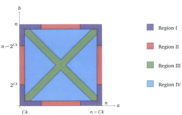
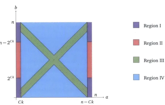
anymore, since this would involve Q(log n) bits of communication and we only have an additional budget of O(log log n). Instead, we undertake a partitioning of the "weight-space", i.e., the set of pairs (lxi,

lyl),

into a finite number of regions. For most of the regions, we reduce the communication task to one of the "Small Set Intersection" or "Small Hamming distance" problems. In the former case, the sizes of the sets are polynomially related to the randomized communication complexity, whereas in the latter case, the Hamming dis-tance threshold is polynomially related to the communication complexity. A naive conversion to protocols for the imperfectly shared setting using the results of [CGMS14] would result in an exponential blow-up in the communication complexity. We give new protocols with im-perfectly shared randomness for these two problems (which may be viewed as extensions of protocols in [BGI14] and [CGMS14]) that manage to reduce the communication blow-up to just a polynomial. This manages to take care of most regions, but not all. To see this, note that any total function h(IxI,

IyI)

can be encoded as a permutation-invariant function f(x,y) and such functions cannot be partitioned into few classes. Our classification manages to eliminate all cases except such functions, and in this case, we apply Newman's theorem to conclude that

(16)

the randomness needed in the perfectly shared setting is only O(log log n) bits (since the in-puts to h are in the range [n] x [n]). Communicating this randomness and then executing the protocol with perfectly shared randomness gives us in this case a private-randomness protocol with communication R(f ) + O(log log n).

1.4 Roadmap of this thesis

In Chapter 2, we give some of the basic definitions and introduce the background material necessary for understanding the contributions of this thesis. In Chapter 3, we introduce our measure m(f) and prove Theorem 1.1.1. In Chapter 4, we show the connections between communication complexity with imperfectly shared randomness and that with perfectly shared randomness and prove Theorem 1.2.1. We end with a summary and some future directions in Chapter 5.

(17)

Chapter 2 Preliminaries

In this chapter, we provide all the necessary background needed to understand the contribu-tions in this thesis.

2.1 Notations and Definitions

Throughout this thesis, we will use bold letters such as x, y, etc. to denote strings in {0, 1}", where the i-th bit of x will be accessed as xi. We denote by lx the Hamming weight of binary string x, i.e., the number of non-zero coordinates of x. We will also denote by A(x,y) the

Hamming distance between binary strings x and y, i.e., the number of coordinates in which x

def

and y differ. We also denote [n] = {1, -- -, n} for every positive integer n.

Very significant for our body of work is the definition of permutation-invariant functions, which we define as follows,

Definition 2.1.1 (Permutation-Invariant functions). A (total or partial) function

f

:{, 1' x

{0, 1} - {0, 1, ?} is permutation-invariant iffor all x,y E {0, 1}n and every bijection i : [n]

-[nl, f (x', y') = f _{(x, y) (where x' is such that x[ = x,(j.}

(18)

Observation 2.1.2. Any permutation-invariantfunction f depends only on IxAyl, IxA-'yl, I-',xAy

and I -x A -y. Since these numbers add up to n, f really depends on any three of them, or in fact

any three linearly independent combinations of them. Thus, we have that for some appropriate functions g, h,

f (x,y) = g(jxj,IyI,Ix A yj) = h(jxj,Iyj, A(x,y))

We will use these 3 representations of f interchangeably throughout this thesis. We will often refer to the slices of f obtained by fixing lxi = a and |y| = b for some a and b, in which case we will

denote the sliced h by either hab(-) or h(a, b, .), and similarly for g.

2.2 Communication Complexity

We define the standard notions of two-way (resp. one-way) randomized commmunication complexity' R(f ) (resp. R-"Y(f )), that is studied under shared/public randomness model (cf.

[KN97]).

Definition 2.2.1 (Randomized communication complexity R(f )). For anyfunction f : {0, I}" x {0, I}" -> {0, 1, ?}, the randomized communication complexity R(f ) is defined as the cost of the

smallest randomized protocol, which has access to public randomness, that computes f correctly on any input with probability at least 2/3. In particular

R(f) = min CC(H)

r

Vx,yE f ,11}" S.t. f (x,y)o ?:

Pr[f(x,y)=f(x,y)]22/3

where the minimum is taken over all randomized protocols H, where Alice and Bob have access to public randomness.

The one-way randomized communication complexity RlWaY(f ) is defined similarly, with the

only difference being that we allow only protocols H where only Alice communicates to Bob, but not other way round.

(19)

Another notion of randomized communication complexity that is studied, is under private randomness model. The work of [CGMS14] sought out to study an intermediate model, where the two parties have access to a i.i.d. samples from a correlated random source p(rs), that is, Alice has access to r and Bob has access to s. In their work, they considered the doubly

symmetric binary source, parametrized by p, defined as follows,

Definition 2.2.2 (Doubly Symmetric Binary Source DSBS(p)). DSBS(p) is a distribution on {0, _{11 x {0, 11, such that for (rs) ~ DSBS(p),}

Pr[r = 1, s = 1] = Pr[r = 0, s = 0] = (1 + p)/4

Pr[r = 1, s = 0] = Pr[r = 0, s = 1] = (1 -p)/4

Note that p = 1 corresponds to the standard notion of public randomness, and p = 0 corresponds to the standard notion of private randomness.

Definition 2.2.3 (Communication complexity with imperfectly shared randomness [CGMS14]).

For any function

f

: {0, 1}" x {0, 1}' --+ {0, 1, ?}, the ISR-communication complexity ISR (f) is defined as the cost of the smallest randomized protocol, where Alice and Bob have access to samples

from

DSBS(p), that computes f correctly on any input with probability at least 2/3. In particular;

ISRP(f) = min CC(I)

VXyeIOl}" s.t. f (x,y)# ?:

Pr[H(x,y)=f (x,y)] 2/3

where the minimum is taken over all randomized protocols H, where Alice and Bob have access to samples from DSBS(p).

def

For ease of notation, we will often drop the subscript p and denote ISR(f) = ISR(f).

We use the term ISR as abbreviation for "Imperfectly Shared Randomness" and ISR-CC for "ISR-Communication Complexity". To emphasize the contrast, we will use PSR and PSR-CC for the classical case of (perfectly) shared randomness. It is clear that if p > p', then

(20)

I SRO (f ) :5 ISR, (f ).

An extreme case of ISR is when p = 0. This corresponds to communication complexity with private randomness, denoted by Rpriv(f). Note that ISR (f) 5 Rpriv(f) for any p > 0. A theorem (due to Newman [New9l]) shows that any communication protocol using public randomness can be simulated using only private randomness with an extra communication of additive O(logn) (both in the 1-way and 2-way models). We state the theorem here for the convenience of the reader.

Theorem 2.2.4 (Newman's theorem [New91]). For anyfunction

f

: {0, I} x {0, 1}" -+ i (any

range Q), the following hold,

Rpriv(f ) 5 R(f ) + O(log n)

R la(f _priv ) 5 R-'"(f ) + O(log n)

here, Rpriv(f ) is also ISRO(f ) and R(f ) is also ISR₁(f).

2.3 Information Complexity

Information complexity2 is an interactive analogue of Shannon's information theory [Sha48]. Informally, information complexity is defined as the minimum number of bits of information that the two parties have to reveal to each other, when the inputs (x,y) e {0, 1}' x {0, 1}" are coming from the 'worst' possible distribution p.

Definition 2.3.1 ((Prior-Free) Interactive Information Complexity; [Bra12]). For any

f

: {0, 1}" x

{0, 1}" -> {0, 1}, the (prior-free) interactive information complexity of

f,

denoted by IC(f), is

defined as,

IC(f) = inf max I(X;HIIY)+I(Y;HIX)

H A

(21)

where, the infimum is over all randomized protocols H such that for all x,y E {0, 1}" such that

f(x,y) # ?, Prp,r1[Hl(x,y) A f(x,y)] 5 1/3 and the maximum is over all distributions y(x,y)

over {0, 1}" x {0, 1}n. [I(A;BIC) is the mutual information between A and B conditioned on C]

We refer the reader to the survey by Weinstein [Weil5] for a more detailed understanding of the definitions and the role of information complexity in communication complexity.

A general question of interest is: what is the relationship between IC(f) and R(f)? It is

known that R(f) 20(c(f)) [Bra12]. Our first result, namely Theorem 1.1.1, shows that for

permutation-invariant functions, R(f) is not much larger than IC(f ).

2.4 Some Useful Communication Problems

Central to our proof techniques is a multi-parameter version of GAP-HAMMING-DISTANCE, which we define as follows.

n _~nn

Definition 2.4.1 (GAP-HAMMING-DISTANCE, GHDcg, GHDabcg). We define GHDabCg as the following promise problem,

1 0

GHD =

if |x= a,y = b and A(x,y) c + g if |x = a,Iy = b and A(x, y) c - g

otherwise

Additionally we define GH a,b,c,g as the following promise problem,

1 0

G n

GHD abc~g

if

lxi

= a,

Iyj

= b and A(x,y) = c + g if lx = a,y = b and A(x,y) = c - g

otherwise

Informally, computing GHDCg is equivalent to the following problem:

(22)

e Bob is given y E {0, 1}" such that

ly

= b

* They wish to distinguish between the cases Az(x,y) > c + g and A(x,y) ; c - g. _n

In the GHDa,b,c,g problem, they wish to distinguish between the cases A(x, y) = c + g or A(x, y) = c - g. Arguably, GHDabcg is an 'easier' problem than GHDnbCg. However, in this

n _n

work we will show that in fact GHDa,b,c,g is not much harder than

GHDa,b,c,g-We will use certain known lower bounds on the information complexity and one-way com-munication complexity of GHDabc for some settings of the parameters. The two main settings of parameters that we will be using correspond to the problems of UNIQUE-DISJOINTNESS and SPARSE-INDEXING (a variant of the more well-known INDEXING problem).

2.4.1 IC lower bound for UNIQUE-DISJOINTNESS

Definition 2.4.2 (UNIQUE-DISJOINTNESS, UDISJ"). UDiSJ" is given by the following promise problem,

1 iflxi= t,Iy= tand

IxAy

=1 UDISJ = 0 if|x = t,jyl = tand

IxAy

=0

otherwise

Note that UDIs t _{is an instance of GHD} ₂_t_{_t}

1I.

Informally, UDIsJ" is the problem where the inputs x,y e {0, I" satisfy lx =

Iy

= t and Alice and Bob wish to decide whether Ix A = 1 or Ix A y = 0 (promised that it is one of them is the case).

Lemma 2.4.3. For all n E N, IC(UDISJ") = )

Proof. Bar-Yossef et al. [BJKSO4] proved that GENERAL-UNIQUE-DISJOINTNESS, that is, unique disjointness without restrictions on |xi,

lyl

on inputs of length n, has information complexity

(23)

a simple padding argument as follows. Given an instance of general UNIQUE-DISJOINTNESS (x', y') E {0, 1}" x {0, I}n. Alice constructs x = x' o 1("- o O"(n+I') and Bob constructs y =

y'o O*(n+I) o ₁("-I I)*. Note that Ix A y = |x' A y'l. Also, we have that x, y e {0, 1}3 , and

lxi =

Iy

= n. Thus, we have reduced GENERAL-UNIQUE-DISJOINTNESS to UDiSj3", and thus the

lower bound of [BJKSO4] implies that IC(UDISJ3") = Q(n).

On top of the above lemma, we apply a simple padding argument in addition to the above lower bound, to get a more general lower bound for UNIQUE-DISJOINTNESS as follows.

Proposition 2.4.4 (Unique Disjointness IC Lower Bound). For all t, w E N,

IC(UDISJit+w) = Q(min {t, w})

Proof. We look at two cases, namely w t and w > t.

Case 1. [w t]: We have from Lemma 2.4.3 that IC(UDJSjiw) > 2(w). We map the in-stance (x',y') of UDISJil to an inin-stance (x,y) of UDISJit+w by the following reduction, x =

x o 1(t-w) o 0(t-w) and y = y' o 0(t~w) o 1(t-w). This implies that IC(UDISJ t+w) = Q ).

Case 2. [w > t]: We have from Lemma 2.4.3 that IC(UDISJFt) = Q(t). As before, we map

the instance (x',y') of UDISJ3L to an instance (x, y) of UDISJft+W by the following reduction,

x = x' o 0(w-t) and y = y' o 0(w-t). This implies that IC(UDISJt+w) = Q(t).

(24)

2.4.2 1-way CC lower bound for SPARSE-INDEXING

Definition 2.4.5 (SPARSE-INDEXING, SPARSEINDn). SPARSEINDn is given by the following promise

problem,

I

if lx= t,jyI =1 and Ix A y| =1

SPARSEIND7 = 0 ifx = t,jy| = 1and IxAy =0

? otherwise

Note that SPARSEINDn is an instance of GHD" .

Informally, SPARSEINDn is the problem where the inputs x,y e {0, 1}" satisfy lx = t and

iyj = 1 and Alice and Bob wish to decide whether Ix A yj = 1 or Ix A y = 0 (promised that one of them is the case).

Lemma 2.4.6. For all a E N, Rl-way(SPARSEIND n) =

Proof. [JKSO8] proved that if Alice is given X E {0, 1}", Bob is given i E [n], and Bob needs to

determine xi upon receving a single message from Alice, then Alice's message should consist of (n) bits, even if they are allowed shared randomness. Using their result, we deduce that

Rl-way(SPARSEIND2n) = Q(n) via the following simple padding argument: Alice and Bob double

the length of their strings from n to 2n, with Alice's new input consisting of (x, RX) while Bob's new input consists of (el, 0), where _ is the bitwise complement of x and e is the indicator vector for location i. Note that the Hamming weight of Alice's new string is equal to n while

its length is 2n, as desired. D

On top of the above lemma, we apply a simple padding argument in addition to the above lower bound, to get a more general lower bound for SPARSE-INDEXING as follows.

Proposition 2.4.7 (SPARSE-INDEXING 1-way CC Lower Bound). For all t, W E N,

(25)

Proof. We look at two cases, namely w t and w > t.

Case 1. [w t]: We have from Lemma 2.4.6 that R1-way(SPARSEIND 2) (w). We map the instance (x',y') of SPARSEIND 2w to an instance (x,y) of SPARSEIND+w by the following

reduc-tion, x = xo 1('-w) and y = y'o 0(-). This implies that Rl-waY(SPARSEINDt+w) Q(w).

Case 2. [w > t]: We have from Lemma 2.4.6 that R-way(SPARSEIND t) = Q(t). We map the

in-stance (x',y') of SPARSEIND2t to an instance (X, y) of SPARSEINDt+W by the following reduction,

x = x' o O(w-') and y = y'o O(wt-). This implies that Rl-waY(SPARS EIND t") E2(t).

(26)

Chapter 3 Coarse Characterization of Information

Complexity

In this chapter, we prove the first of our results, namely Theorem 1.1.1, which we restate below for convenience of the reader.

Theorem 1.1.1. Let f : {0, 1}" x {0, 1}' -- {0, 1, ?} be a (total or partial) permutation-invariant

function. Then,

m(f) IC(f) R(f) poly(m(f ))+ O(log n).

where m(f ) is the combinatorial measure we define in Definition 3.2.1.

3.1 Overview of proof

We construct a measure m(f ) such that m(f ) 5 IC(f ) 5 R(f ) 5

O(m(f

)4)+ O(log n). In order to do this, we look at the slices of

f

obtained by restricting lxi and

lyl.

As in Observation 2.1.2, let hab(A(x,y)) be the restriction of h to lx = a and

jyl

= b. We define the notion of a jump

in ha,b as follows.

Definition 3.1.1 (Jump in ha,b)- (c, g) is a jump in ha,b if ha,b(c+g)

#

ha,b(c-g), both ha,b(c+g),

(27)

Thus, any protocol that computes

f

with low error will in particular be able to solve a

GAP-HAMMING-DISTANCE _{problem GHD,,blc1g as in Definition 2.4.1. Thus, if}_(c,_{g) is a jump for ha,b,} then IC(GHDabcg) is a lower bound on IC(f). We will prove lower bounds on IC(GHDac)_a, _~ a,

b,c,g

for any value of a, b, c and g by obtaining a variety of reductions from UNIQUE-DISJOINTNESS, and then our measure m(f) will be obtained by taking the largest of these lower bounds for

_n

IC(GHDa,b,c,g) over all choices of a and b and jumps (c, g) in ha,b

Suppose m(f) = k. We construct a randomized communication protocol with cost 6(k4) +

O(log n) that computes f correctly with low constant error. The protocol works as follows: First, Alice and Bob exchange the values lxi and ly, which requires O(log n) communica-tion (say, lxi = a and Iy = b). Now, all they need to figure out is the range in which A(x, y) lies (note that finding A(x, y) exactly can require Q(n) communication!). Let Y (ha,b) =

{(c1, g1), (c2, g2), --' , (cm, g.)} be the set of alljumps in ha,b. Note that the intervals [ci -gi, ci +

gi] are all pairwise disjoint. To compute ha,b(x,y)), it suffices for Alice and Bob need to

resolve each jump, that is, for each i E [M], they need to figure out whether A(x, y) > c + g or A(x, y) c - g. We will show that any particular jump can be resolved with a constant

prob-ability of error using O(k3) communication, and the number of jumps m is at most 20(k) log n.

Although the number of jumps is large, it suffices for Alice and Bob to do a binary search through the jumps, which will require them to resolve only O(k log log n) jumps each requiring

0(k3) communication. Thus, the total communication cost will be 6(k4

) + O(log n).'

3.2 Proof of Theorem 1.1.1

As outlined earlier, we define the measure m(f ) as follows.

Definition 3.2.1 (Measure m(f )). Given a permutation-invariantfunction f : {o, 1}" x {O, I}" -+

'We will need to resolve each jump correctly with error probability of at most 1/ (kloglogn). And for that we will actually require O(k3 log k log log log n) communication. So the total communication is really O(k4 log k

(28)

{0, 1, ?} and integers a, b, s.t. 0 5 a, b < n, let ha,b : {0, ---, n} -3 {0, 1, ?} be the function given

by ha,b(d) = f (x,y) if there exist x,y with lxi = a, |y| = b, A(x,y) = d and ? otherwise. (Note. by

permutation invariance of f, ha,b is well-defined.) Let Y (ha,b) be the set of jumps in h a,b, defined as follows, def f(ha,b) =(c, g): ha,b(c - g), ha,b(C + g) E {0, 11 ha,b(c - g) # ha,b(c + g) ViE(c-g,c+g)

_:

_{ha,b(i)=? f} def ₁

C a,be[n] max max I m lmin{cn-c})}_g _g

(c,g)EY(hab)

where C is a suitably large constant (which does not depend on n).

We will need the following lemma to show that the measure m(f) is a lower bound on IC(f).

n

Lemma 3.2.2. For all n, a, b, c, g for which GHDa,b,c,g is a meaningful problem2_{, the following}

lower bounds hold,

IC(GHD"bc) I(GHDa,b,c,g) IC(GHDa,b,c,g) 1 C min {a, b, c, n - a, n - b, n - c} 1og (min {c n-c}

Next, we obtain randomized communication protocols to solve

GHDbCg-Lemma 3.2.3. Let a b 5 n/2. Then, the following upper bounds hold

R(GHD n,c,g)

R(GHD _n,c,g)

+log

= 0(min ( )2, (nC)2

2_{that is, a, b}₅

n and c + g and c - g are achievable hamming distances when xI = a and ly = b.

Then, we define m(f) as follows.

(29)

We defer the proofs of the Lemmas 3.2.2 and 3.2.3 to Section 3.3. For now we will use these lemmas to prove Theorem 1.1.1. First, we show that each jump can be resolved using O(m(f )3)

communication.

Lemma 3.2.4. Suppose m(f) = k, and let

lxi

= a and |y| = b. Let (c, g) be any jump in

ha,b-Then the problem of GHDCg, that is, deciding whether A(x, y) ;> c + g or A(x, y) c - g can

be solved, with a constant probability of error; using 0(k3) communication.

Proof. We can assume without loss of generality that a b n/2. This is because both Alice and Bob can flip their respective inputs to ensure a, b n/2. Also, if a > b, then we can flip

the role of Alice and Bob to get a b n/2.

Since a _{b 5 n/2, from definition of m(f ) in Lemma 3.2.2 we have that,}

min a n - c} 5 O(k)

We consider two cases as follows.

Case 1. (clg) O(k) or ((n-c)/g) 5 O(k): In this case we have, from part (ii) of Lemma 3.2.3, a randomized protocol with cost 0 (min {(c/g)2, ((n - c)/g)2}) = O(k2).

Case 2. (a/g) 5 O(k): In this case, we will show that ((a/g)2(log(b/a)+log(a/g))) <

O(k3_). _Clearly,

(a/g)2 O(k2_{) and log(a/g)} _{0(logk). We will now show that in fact} log(b/a) O(k). From part (ii) of Lemma 3.2.2 we know that either log(c/g) O(k) or log((n - c)/g) 5 O(k). Thus, it suffices to show that (b/a) 5 0 (min {(c/g), ((n -c)/g)}). We know that b - a + g c 5 b + a - g. The left inequality gives (b/a) 5 (c + a - g)/a =

(c/g).(g/a) + 1 - (g/a) 5 0(c/g) (since g/a 5 1). The right inequality gives ((n - b)/a) 5

((n - c)/g).(g/a) + 1 - g/a 0((n - c)/g). Since b 5 n/2, we have (b/a) 5 ((n - b)/a)

0((n - c)/g). D

Next, we obtain an upper bound on If (ha,b)I, that is, the number of jumps in

ha,b-Lemma 3.2.5. For any function

f

: {O, 1}" x {0, In -- {0, 1} with m(f) = k, the number of jumps in ha,b is at most 20(k) log n.

(30)

Proof. Let y = {(ci, gl), - -- ,(c, g,,)} be the set of all jumps in ha,b. Partition Y into U 2, Y

where = {(c, g) E

Y

: c 5 n/2} and Y2 = {(c, g) E

Y

: c > n/2}. From second part in Lemma 3.2.2 we know the following:

V(c, g) E : log (. :5 O(k) that is, g c2-0(k)

V(c, g) E Y2 l og n-c )5 O(k) that is, g (n - c)2-0(k)

g -9

Let

Y,

= {(c1, g1),- -, (c,, g,)}, where the ci's are sorted in increasing order. We have that

ci + gi 5 ci+1 - gi+1 for all i. That is, we have that ci(1 + 2--0()) ci, 1(1 - 2-0()), which

gives that ci1 ci(1 + 2-0(k)). Thus, n/2 - c!, ! cl1( + 2-0(k))P, which gives that yi

I

=

p 5 20(k) log n. Similarly, by looking at n - ci's in 12, we get that IY21 5 ₂0(k) log n, and thus,

I/I

5 2O(k)log n. I

We now complete the proof of Theorem 1.1.1.

-n

Proof of Theorem 1.1.1. Any protocol to compute f also computes GHDa,b,c,g for any a, b and any jump (c, g) E V(ha,b). Consider the choice of a, b and a jump (c, g) e 1(ha,b) such

that the lower bound obtained on IC(GH-D ng) through Lemma 3.2.2 is maximized, which by definition is equal to m(f ) (after choosing an appropriate C in the definition of m(f)). Thus, we have m(f) IC(GHDa,b,c,g) IC(f).

We also have a protocol to solve f, which works as follows: First Alice and Bob exchange lxi = a and Iy = b, requiring O(log n) communication. From Lemma 3.2.5, we know that the number

ofjumps in ha,b is at most 20('(f)) log n, and so Alice and Bob need to do a binary search through

the jumps, resolving only 0(m(f)loglog n) jumps, each with an error probability of at most

0(1/m(f)loglog n). This can be done using O(m(f)3_{) communication}3 _{(using Lemma 3.2.4).} Thus, the total amount of communication is R(f ) 5 0(m(f )4_{) + O(log n)}4_{. All together, we}

3_{Here, O(m(f)}3₎₌_O(m(f)3 _{log m(f)logloglogn).}

4_{Here O(m(f}_{)4) =}

(31)

have shown that,

m(f) IC(f ) R(f ) O(m(f )4) + O(log n)

Remark. It is a valid concern that we are hiding a log log n factor in the O(m(f)4) term. But this is fine because of the following reason: If m(f ) (log n)1/5, then the O(log n) term is the

dominating term and thus the overall communication is O(logn). And if m(f) > (log n)11 , then log m(f) = Q(loglogn), in which case the O(m(f)4) is truly hiding only polylog m(f)

factors.

In the following section, we prove the main technical lemmas used, namely 3.2.2 and 3.2.3.

3.3 Results on Gap Hamming Distance

In this section, we prove lower bounds on information complexity (Lemma 3.2.2), and up-per bounds on the randomized communication complexity (Lemma 3.2.3) of

GAP-HAMMING-DISTANCE.

Lower bounds

We will prove Lemma 3.2.2 by getting certain reductions from UNIQUE-DISJOINTNESS (namely Proposition 2.4.4). In order to do so, we first prove lower bounds on information complex-ity of two problems, namely, SET-INCLUSION (Definition 3.3.1) and SPARSE-INDEXING (Defini-tion 2.4.5). We do this by obtaining reduc(Defini-tions from UNIQUE-DISJOINTNESS.

Definition 3.3.1 (SETINC" ). Let p < q < n. Alice is given X E {0, 1I" such that lxi = p and Bob

is given y E {0, 1}" such that |y| = q and they wish to distinguish between the cases Ix A y| = p and Ix A y| = p - 1. Note that SETINC" _{pq .3}is the same as _Ue_sam) GHD_ _,E _NqICSEINC1..

(32)

Proof. We know that IC(UDISJt+w) Q(min(t, w)) from Proposition 2.4.4. Note that UDISJ t+w 2 tt

is same as the problem of GHD w .2t If we instead think of Bob's input as complemented, we

2t+w 2t+w

get that solving GHD _2t, is equivalent to solving GHDL+wW , which is same as SETINC2t+.

t~tt-l~ t~+WW+,11t,t+w'

Thus, we conclude that IC(SETINCn , w (min(t, w)). El

t,t+w

Proposition 3.3.3 (SPARSE-INDEXING lower bound). Vt E N, IC(SPARSEIND 1 2t (t

Proof. We know that IC(UDisj_kt/3Jt 1') Q(t) from Proposition 2.4.4. Recall that SPARSEIND _SP _EN 2+is

2t i an instance of GHD 2t1 . Alice uses x to obtain the Hadamard code of x, which is X e {o, 1}

such that X(a) = a -x (for a e {0, 1}t+1). On the other hand, Bob uses y to obtain the indicator vector of y, which is Y E {0, 1}2t+ such that Y(a) = 1 iff a = y. Clearly JYJ = 1. Observe that,

lX

= 2' and X(y) = y- x is 1 if JxAy = 1 and 0 if JxAyl = 0. Thus, we end up with an instance

of SPARSEIND 2t+. Hence IC(SPARSEIND +) IC(UDisJt 1) Q(t). El

2t 2t t/3

We now state and prove a technical lemma that will help us prove Lemma 3.2.2.

Lemma 3.3.4. Let a b 5 n/2. Then, the following lower bounds hold,

(i) _{IC(GHDa,b,c,g) 2} _(mIgI+ag

})

(ii) IC(GHDambcg)

r

(n

{

a+b-c c+b-a

(iii) IC(GHDa,b,c,g) Q mi {log , log (

Proof. We prove the three parts of the above lemma using reductions from UDIsJ, SETINC and SPARSEIND respectively. Note that once we fix lx = a and Iy = b, a jump (c, g) is

meaning-ful only if b - a + g c 5 b + a - g (since b - a A(x, y) b + a). We will assume that c = b + a - g(mod 2), so that c + g and c - g will be achievable Hamming distances.

Proof of (i). We obtain a reduction from UDISJ t for which we know from Proposition 2.4.4 that IC(UDISJ t) Q(t). Recall that UDISJ t is same as GHDt . Given any instance of

3t 3gt

(33)

we need to append (a - g t) l's to x and (b - g t) l's to y. This will increase the Hamming distance by a fixed amount which is at least (b - a) and at most (b + a - 2g t). Also, the

number of inputs we need to add is at least ((a - gt) + (b - gt) + (c - g(2t - 1)))/2 '. Thus,

we can get a reduction to GHDabcg if and only if,

(b-a) c-g(2t -1) b+a-2gt

n 3gt + (a -gt) + (b - gt) + (c - g(2t -1))

2

The constraints on c give us that 2g t c - (b - a) + g and c 5 b + a - g (recall that this is

always true). The constraint on n gives that g t n - (a + b + c + g)/2, which is equivalent to

t<n-a-b + n-c-g

- 2g 2g

Thus, we can have the reduction work by choosing t to be

t=min{ c-b+a+g n-c-g . c-b+a n-c

I 2g 2g g g

(since n a + b) and thus we obtain

- n

D S t) > Qc- _{b + a n - cf}

IC(GHDa,b,c,g) IC(UDISJ) 2 ( min

{

gg

Proof of (ii). We obtain a reduction from SETINC7W (where m = 2t + w) for which we know

from Proposition 3.3.2 that IC(SETINC7') Q(min {t, w}). Recall that SETINC is same as GHD . Given an instance of GHD , we first repeat the instance g times to get an instance of GHDg Now, we need to append (a-g t) l's to x and (b-g t-gw) l's

to y. This will increase the Hamming distance by a fixed amount which is at least I b - a - gwl

sWe will be repeatedly using this idea in several proofs. The reason we obtain the said constraints is as follows:

Suppose Alice has to add A 1's to her input and Bob has to add B 1's to his input. Then the hamming distance increases by an amount C such that |A -B 5 C 5 A +B. Also, the minimum number of coordinates that need to

(34)

and at most (b - g t - gw) + (a - g t). Also, the number of inputs we need to add is at least

((a -gt)+(b -gt -gw)+(c -g(w +1)))/2. Thus, we can get a reduction to GHD _a,b,c,gc if and

only if,

Ib-a-gwl 5 c-g(w+1) b+a-2gt -gw (b - gt - gw) + (a - gt) + (c - gw - g)

n 22gt +gw+2 2

The left constraint on c requires c max{b-a +g,2gw -(b -a)+g}. We know that c b - a + g, so the only real constraint is c 2gw - (b - a) + g, which gives us that,

c + b -a - g

2g

The right constraint on c requires c b + a - 2g t + g, which gives us that,

t<a+ b-c+g 2g

Suppose we choose t = 2g g. Then the constraint on n is giving us that,

a+b+c-g _ a+b-c+g + b+c-g

2 2 2

We already assumed that a b n/2, and hence this is always true.

Thus, we choose t = a+b-c+g and w _2g = Cga- ₂ , and invoking Proposition 3.3.2, we get,

I( n C,, a+b-c c+b-a)

IC(GHD a,b,c,g IC(SETINC t w) min({ t, w}) 2Q (min ,

b-cc

a~b~cg ~ g gJ

Proof of (iii). We obtain a reduction from SPARSEIND t

+ for which we know from

Proposi-2t tion 3.3.3 that IC(SPARSEIND 1) Q

G(t). Recall that SPARSEIND 2t is same as GHD 2,

2t+1

which is equivalent to GHD 1 2t2 1 (if we flip roles of Alice and Bob). Given an instance of

2t+1 -g2t+l

GHD , we first repeat the instance g times to get an instance of GHD gg2 g2tg* Now, we

(35)

by a fixed amount which is at least lb - g2' - a + gI and at most (b - g2' + a - g). Also, the

number of inputs we need to add is at least ((a - g) + (b - g2') + (c - g2'))/2. Thus, we can

get a reduction to GHD ,b,c,g if and only if,

b - g2'-a+ g 15 c - g2' < (b - g2' +a - g)

n !g2t 1 + (a -g)+(b -g2')+(c -g2')

2

The left constraint on c requires c max {b - a + g, 2g2' - b + a - g}. Since c ! b - a + g anyway, this only requires 2g 2' < c + b-a + g. The right constraint on c requires c 5 b + a -g

which is also true anyway. The constraint on n is equivalent to,

a+b+c-g _ n-a-b n-c-g

g2t_En- ₌ ₊

2 2 2

Thus, we choose t such that,

t = min log2 c+ba + g102 (n- )} min -,nC

I 2g 2g g g

and invoking Proposition 3.3.3, we get,

IC(GHDb) n IC(SPARSEIND 2') Q(t) Q min log2(iC), log2(n-C)})

FD

We are now finally able to prove Lemma 3.2.2.

Proof of Lemma 3.2.2. Assume for now that a b 5 n/2.

Lemma 3.3.4, we know the following,

IC(GHDab,c,g)

n

IC(GHDa,b,c,g)

From parts (i) and (ii) of

S(min cn-b+a, nf-c

n (min

{

a+b-c c+ b-a

(36)

Adding these up, we get that,

IC(GHDab,c,g (min{c-b _G_un +a _, n c + min a+b-c c+b-a_,

Since min{A,B} +min{C,D} = min{A+ C,A+D,B + C,B +D}, we get that,

I C (GH-D) _{C(H a}_,b,cn _g)

(

min 2a 2c n+a+b-2c n+b-a, ,,

For the last two terms, note that, n + a + b - 2c n - c (since a + b c) and n + b - a : n

(since b a). Thus, overall we get,

IC(GHDab~cg) , b(n

{

1,

Note that this was assuming a b 5 n/2. In general, we get,

IC(GHDbcg) . (min{a, b, c, n-a, n - b, n - cl

[We get b, (n- b), (n -a) terms because we could have flipped inputs of either or both of Alice and Bob. Moreover, to get a b, we might have flipped the role of Alice and Bob.]

The second lower bound of IC(GHDabc) 2 (log (minlc f-c) follows immediately from part

(iii) of Lemma 3.3.4.

We choose C to be a large enough constant, so that the desired lower bounds hold. El

Upper bounds

We will now prove Lemma 3.2.3.

Communication complexity of permutation-invariant functions