Integration of routing into a resource-constrained project scheduling problem

HAL Id: hal-01948603

https://hal.archives-ouvertes.fr/hal-01948603

Submitted on 4 Feb 2020

HAL is a multi-disciplinary open access

archive for the deposit and dissemination of

sci-entific research documents, whether they are

pub-lished or not. The documents may come from

teaching and research institutions in France or

abroad, or from public or private research centers.

L’archive ouverte pluridisciplinaire HAL, est

destinée au dépôt et à la diffusion de documents

scientifiques de niveau recherche, publiés ou non,

émanant des établissements d’enseignement et de

recherche français ou étrangers, des laboratoires

publics ou privés.

project scheduling problem

Philippe Lacomme, Aziz Moukrim, Alain Quilliot, Marina Vinot

To cite this version:

Philippe Lacomme, Aziz Moukrim, Alain Quilliot, Marina Vinot.

Integration of routing into a

resource-constrained project scheduling problem. EURO Journal on Computational Optimization,

Springer, 2019, 7 (4), pp.421-464. �10.1007/s13675-018-0104-z�. �hal-01948603�

Integration of Routing into a Resource-Constrained

Project Scheduling Problem

Philippe Lacomme

_{, Aziz Moukrim}

_{, Alain Quilliot}

_{Marina Vinot}

63177 Aubière Cedex, France.

b _{Sorbonne Universités, Université de Technologie de Compiègne, (Heudiasyc UMR CNRS 7253),} CS 60 319, 60203 Compiègne France.

ARTICLE INFO ABSTRACT

Article history: Received: Accepted: Available: Keywords: Routing Scheduling RCPSP

The Resource-Constrained Project Scheduling Problem (RCPSP), one of the most challenging combinatorial optimization scheduling problems, has been the focus of a great deal of research, resulting in numerous publications in the last decade. Previous publications focused on the RCPSP, including several extensions with different objectives to be minimized and constraints to be checked. The present work investigates the integration of the routing, i.e., the transport of the resources between activities into the RCPSP, and provides a new resolution scheme. The two sub-problems are solved using an integrated approach that draws on both a disjunctive graph model and an explicit modeling of the routing. The resolution scheme takes advantage of an indirect representation of the solution to define both the schedule of activities and the routing of vehicles. The routing solution is modeled by a set of trips that define the loaded transport operations of vehicles that are induced by the flow in the graph. The numerical experiments prove that the models and the methods introduced in this paper are promising for solving the RCPSP with routing.

1

Introduction

1.1. Resource-Constrained Project Scheduling Problem

The Resource-Constrained Project Scheduling Problem (RCPSP) represents a challenging research problem that has been widely studied over the past decades. This problem is composed a set of activities, 𝑉 = {0, . . . , 𝑛 + 1 }, with durations, 𝑝 = (𝑝0, . . . , 𝑝𝑛+1), where 𝑛 is the number of non-dummy activities. All this activities define the

project. There are two dummy activities, 0 and 𝑛 + 1, such that 𝑝0= 𝑝𝑛+1= 0. These activities 0 and 𝑛 + 1

correspond to the “project start”, which is the predecessor of all activities, and to the “project end”, which is the successor of all activities, respectively. The set of non-dummy activities is identified by 𝐴 = {1, … , 𝑛}. The activities are linked by two kinds of constraints, the precedence constraints (one activity 𝑗 cannot start before all its predecessors have been achieved) and the resource constraints induced by the resource exchanges (an activity requires resources to be achieved). A schedule of the RCPSP can be represented as a vector of activity start times, 𝑆 = (𝑆0, . . . , 𝑆𝑛+1), where 𝑆𝑖 ∈ ℕ, with the associated vector of activity completion times, 𝐶 =

(𝐶0, . . . , 𝐶𝑛+1). The precedence graph is denoted 𝐺 = (𝑉, 𝐸), where nodes in 𝑉 are activities and edges in 𝐸 are

precedence relations. For each activity 𝑖 ∈ 𝑉, all outgoing arcs (𝑖, 𝑗) ∈ 𝐸 are weighted by its duration 𝑝𝑖. If there

are arcs (𝑖, 𝑗) ∈ 𝐸, then 𝐶𝑖= 𝑆𝑖+ 𝑝𝑖≤ 𝑆𝑗 since activity 𝑗 has to be scheduled after activity 𝑖. Each activity requires

some amount of renewable resources. The number of project resources is denoted as 𝑞 and the set of resource is 𝑅 = {𝑅1, . . . , 𝑅𝑞}. The activity resource requirement 𝑏𝑖𝑘∈ ℕ means that activity 𝑖 requires 𝑏𝑖𝑘≤ 𝐵𝑘 resource

units of resource 𝑘 during its execution such that 𝐵𝑘 denotes the availability of resource 𝑘. The longest path from

0 to 𝑛 + 1 in graph 𝐺(𝑉, 𝐸) corresponds to the critical path.

Because the RCPSP is an extension of the job-shop, it is an NP-hard problem (see Blazewicz et al. (1983) and Brucker et al. (1999) for details on complexity). Several surveys are available including, but not limited to, the survey of Herroelen et al. (1998), of Brucker et al. (2000), of Kolisch and Padman (2001), of Weglarz (1999) in the book on Project Scheduling, of Demeulemeester and Herroelen (2002) and of Hartmann and Briskorn (2010). Note that Brucker (1999) provided a classification scheme for the relationships between RCPSP and machine scheduling. More recently, Kolisch and Padman (2001) introduced a survey of heuristic methods for the different classes of project scheduling problems.

1_{Corresponding author. e-mail addresses: placomme@isima.fr (P. Lacomme), aziz.moukrim@utc.fr (A. Moukrim),}

Numerous models and several formulations have been introduced including a formulation based on forbidden sets introduced by Alvarez-Valdés and Tamarit (1993), the aggregated time indexed formulation (Pritsker et al. 1969), the time-indexed formulations with step variables of Pritsker and Watters (1968), the compact event-based formulation that has been used to address scheduling problems with machines (for example, Dauzère-Pérès and Lasserre (1995)), and the recent flow formulation of Artigues et al. (2003).

A RCPSP solution can be linked to the network flow theory (Ahuja et al., 1993) since it involves circulation of resources that can be goods, people or energy, for example. RCPSP resolution based on flow approaches received attention in Artigues and Roubellat (2000) and Artigues et al. (2003). As stressed by Artigues et al. (2003), a solution of the RCPSP can be modeled by an activity-on-node (AON)-flow network where the earliest starting time (S) of activities is computed using a longest path algorithm and where disjunctions are resolved by a flow definition. An AON-flow network representation permits to model the circulation of resources in a graph where nodes correspond to activities and arcs correspond to resources transferred (Artigues et al., 2003).

1.2. Problem of interest: RCPSPR

The RCPSP with routing (RCPSPR) is an extension of the RCPSP where the resource transport between activities must now be achieved by a limited fleet of vehicles. The problem consists of finding a feasible schedule of minimal duration 𝐶𝑚𝑎𝑥 by assigning a starting time to each activity (classical RCPSP) as well as assigning a vehicle to each

transport of resources with a starting time such that the precedence relations, the resource availabilities and the vehicle capacities are respected. Such problems occur in practice when a resource is physically moved from one location to another (e.g., when a crane has to be transported between construction sites or for scaffolding moved between sites to complete a project). In contrast to the classical RCPSP, no article appears to have dealt with this extension so far. This paper focuses on the case of one resource 𝑞 = |𝑅| = 1 and, therefore, 𝑏𝑖𝑘= 𝑏𝑖.

The routing problem consists of scheduling trips for a set of vehicles 𝑇 = {1, . . . , 𝑣 } sorted in descending order of capacity 𝑐𝑢, 𝑢 ∈ {1, … , 𝑣} with a loaded transportation time 𝑡𝑖𝑗𝑢𝑥 from activity 𝑖 to 𝑗 with a vehicle 𝑢 loaded with 𝑥

units of resources and an unloaded transportation time 𝑒_𝑖𝑗𝑢 from activity 𝑖 to 𝑗. Since the transportation times are vehicle-independent and vehicle load-independent, 𝑡_𝑖𝑗𝑢𝑥= 𝑡𝑖𝑗 and 𝑒𝑖𝑗𝑢 = 𝑒𝑖𝑗. The vehicle is responsible for the

transport (transfer) of the resource. An activity 𝑗 is defined by a starting time 𝑆_𝑗 with a completion time 𝐶_𝑗= 𝑆_𝑗+ 𝑝𝑗 and resource supplies that meet the requirement 𝑏𝑗. An activity can only start when a total amount 𝑏𝑗 of resources

has been transferred from activities to activity 𝑗. Each transport operation 𝑇(𝑖,𝑗,𝑢,𝑥) = (𝑃(𝑖,𝑗,𝑢,𝑥) , 𝐷(𝑖,𝑗,𝑢,𝑥) ) from

activity 𝑖 to 𝑗 is fully defined by a pickup operation 𝑃(𝑖,𝑗,𝑢,𝑥) and a delivery operation 𝐷(𝑖,𝑗,𝑢,𝑥) . A pickup operation

and a delivery operation are defined by:

 A departure time and an arrival time of the vehicle, 𝐵(𝑖,𝑗,𝑢,𝑥) and 𝐴(𝑖,𝑗,𝑢,𝑥) , respectively;

 A quantity of resource (pickup or delivery) 𝑥;  A vehicle 𝑢 assigned to the transport.

In this paper, a transport operation, 𝑇(𝑖,𝑗,𝑢,𝑥) is a couple of pickup/delivery operations and 𝐵(𝑖,𝑗,𝑢,𝑥) is the departure

time of the vehicle (starting time of the transport operation) (Fig. 1). A similar remark holds for the arrival time 𝐴(𝑖,𝑗,𝑢,𝑥) of the vehicle 𝑢 on activity 𝑗. The earliest starting time of one activity 𝑆𝑗 depends on the arrival time of

all vehicles, i.e., of all delivery operations.

Earliest starting time of the activity

Si

Earliest finishing time of the activity

Ci

waiting time of the x resources

in the output buffer Activity i

Activity j

Activity k

waiting time of the y resources

in the output buffer

B(i,j,u,x)

A(i,j,u,x)

A(k,j,v,y)

Earliest starting time of the activity

Sj

Earliest finishing time of the activity

Cj Sk Ck B(k,j,v,y) T(k,j,v,y) vehicle u vehicle u

Waiting time of vehicle u

waiting time of the x resources

in the input buffer

Fig. 1. Coordination between transport operations and activities

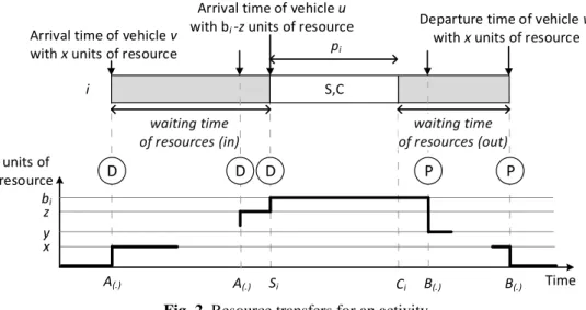
The difference between 𝑆𝑗 and 𝐴(𝑖,𝑗,𝑢,𝑥) defines the total waiting time of the 𝑥 units of resource in a buffer (Fig.

between the completion time 𝐶_𝑖 and the departure time 𝐵_{(𝑖,𝑗,𝑢,𝑥)} models a waiting time of resources in an output buffer.

The total amount of resources available upstream of activity 𝑖 is an increasing function (which depends on the delivery operations) before the starting time of activity 𝑖, and a decreasing function that models the remaining resources after completion of 𝑖 and before the pickup operations (Fig. 2).

Fig. 2. Resource transfers for an activity

The vehicles are also submitted to waiting times between two successive transport operations. Because no buffer constraints are addressed, the waiting time of a vehicle depends only on the activity finishing times and is defined by the difference between the arrival time of the vehicle on one activity (to deliver some resources) and the vehicle departure time (which is equal to the activity finishing time), as can be seen in Fig. 2. The vehicle can immediately leave after a delivery operation on an activity, the resources are stored or used by the activity. To reduce the waiting times, an integrated approach should be developed to solve the problem, with the scheduling, the routing and the assignment of vehicles for each transport operation. Nevertheless, the waiting times are not taken into account explicitly in the objective function in this paper, and the objective function addresses the makespan minimization. In this paper, the resources are not allowed to make trips and only direct resource transfers are permitted to address routing problems with perishability or security (service quality) constraints where mistakes concerning vehicle unloading operations must be fully eliminated.

1.3. Classification

Numerous classifications of resource types have been introduced for years by Brucker et al. (1999) and Demeulemeester and Herroelen (2002) and make a strong distinction between renewable, non-renewable, and partially renewable resources. Taking advantages of the classification recently defined by Krüger and Scholl (2009), the problem concerns a problem with:

 A 1st _{tier resource that must be transferred at a certain time and that models a personnel, a tool, a material or}

any heavy machinery required to achieve an activity.

 A 2nd _{tier resource that supports the transfer of the 1}st _{tier resource.}

The type of 2nd _{tier resource transfer is assumed to be a physical transfer that is characterized by moving the 1}st

tier resource from one location to another. The physical transfer is assumed to be achieved by a material handling resource denoted below the vehicle (without loss of generality) so as to be consistent with the widespread current usage in routing and a transfer defined as a transportation problem. Consequently, a RCPSP satisfying the previous definition can also be denoted RCPSPR (with Routing) since only physical transfers are addressed for 1st _tier

resources by 2nd _{tier resources.}

2

Scheduling/Routing context

In recent years, a tremendous amount of research has been devoted to production and transportation sub-problems and, as highlighted by Chen (2010), integrated production and transport models at a detailed scheduling level are fairly recent and the majority of models attempts to jointly optimize operation-by-operation production and transport. The RCPSP with routing (RCPSPR) falls into the category of production and transportation scheduling

S,C Arrival time of vehicle v

with x units of resource

Time units of

resource

x

Departure time of vehicle w with x units of resource

y z

i

bi

Arrival time of vehicle u with bi -z units of resource

D D D P P Si Ci pi A(.) waiting time of resources (in) waiting time of resources (out) A(.) B(.) B(.)

problems (PTSP), which are key operational functions in a supply chain since it is critical to jointly integrate these two planning and scheduling functions in a coordinated manner.

2.1. Modeling transport in the scheduling problem

Several scheduling problems encompass some extensions with transportation constraints involved by critical handling resources, including, for example, the flexible job-shop scheduling problem with transport (see Zhang et al (2012)), the job-shop with transport (see Knust (1999), Lacomme et al. (2007), Afsar et al. (2016)), the Flexible Manufacturing Systems (FMS) (Caumond et al., 2009), the HSP (Hoist Scheduling Problem) (Honglin et al., 2016; Adnen and Mohsen, 2016; Chtourou et al., 2013) or the RCPSP with transport (see Quilliot and Toussaint (2012)). Two recent papers (Weiss and Schwindt, 2016;Poppenborg and Knust, 2016) addressed an integrated scheduling and routing problem with time transfer constraints in RCPSP-like problems. However, in these studies, the routing is not explicitly modeled with a fleet of vehicles.It is commonly accepted that most of the scheduling approaches take advantage of a modeling based on a graph that is derived from the disjunctive graph of Roy and Sussmann (1964). This model has been extended to scheduling problems with transport (for the job-shop by Lacomme et al. (2007) and Zhang et al. (2012)), where transport operations are modeled by a vertex with disjunctive arcs between each operation that requires the same resource (vehicle).

The integration of transport constraints into scheduling problems can be modeled in two possible ways considering two situations. The first one consists of physically moving resources from one location to another (modeling heavy-machine transport or specialists flying around the world, for example). The second one consists of models based on time-lags between machines where time-lags are a variant of transfer time. Time-lags are associated with activities, whereas setup times are associated with resources. It should be noted that setup times can depend on both the schedule and on the resource management.

Minimal time-lags between activities are commonly used to model a minimal delay and can depend on the consecutive activities. If explicit vehicle management is not required, this approach provides an efficient modeling of transport and can also be relevant in problems where the vehicle fleet is large enough to assume that a transport can be achieved with no delay after the end of one activity. The problem studied by Poppenborg and Knust (2016), referred to as RCPSP with transfer times belongs to this approach. The integrated problem studied in this paper extends this recent paper by taking vehicle management into account.

Maximal time-lags between activities can lead to a maximal delay for the transport and are commonly used in pickup and delivery problems where a maximal riding time is defined. It is important to note that two widely used approaches for trip evaluation introduced first in Cordeau and Laporte (2003) and, second, in Firat and Woeginger (2011) take advantage of such modeling approaches, as reported in Chassaing et al. (2015).

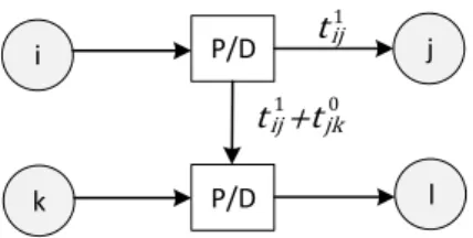
Explicit transport modeling depends on the vehicle capacity and, in the specific situation of unary vehicle capacity (which means that the vehicle cannot achieve more than one transport operation at a time), a trip is a sequence of operations defined by a Pickup operation (𝑃), a Delivery operation (𝐷), a Vehicle (𝑉) and a quantity transported (𝑞), i.e., by a quadruplet (𝑃, 𝐷, 𝑉, 𝑞). Hence, a solution of the routing problem consists in defining the disjunctions between the transport operations (square node in Fig. 3).

Fig. 3. Explicit representations of transport

operations with a single capacity vehicle

Depending on the problem, the transportation time can be job-dependent and vehicle load-dependent and can be denoted 𝑡_𝑖𝑗𝑥. A similar notation holds for the unloaded vehicle transport denoted 𝑡𝑖𝑗0 (commonly denoted 𝑒𝑖𝑗= 𝑡𝑖𝑗0).

As stressed by Lacomme et al. (2013), the disjunctive arc between two transport operations is modeled by an arc with value 𝑡𝑖𝑗1 + 𝑡𝑗𝑘0, which corresponds to a loaded transport

from 𝑖 to 𝑗 and an unloaded transport from 𝑗 to 𝑘 Fig. 3. Such approaches have been used in the flexible flow-shop resolution by Zhang et al. (2012) and in the job-shop by Lacomme et al. (2010). For the RCPSP-like problem, as pointed out by Krüger and Scholl (2009), resource transfers between activities are known to be highly relevant in practice but most research papers neglect them.

2.2. Routing in scheduling problems

Previous related studies only focused on transport with scheduling (including the job-shop, for example) since the transport was only used to check some extra constraints in scheduling. However, no previous study exists where the transport is modeled using classical approaches taken from the routing community. It is unfortunate that

i P/D j k P/D l 0

t

t

t

classical routing approaches are not widely used in integrated problems with scheduling, in view of the huge number of efficient routing approaches that tackle routing with some extra constraints. Numerous approaches to routing problems take advantage of indirect solution representations and are consistent with the same trend of widespread approaches in scheduling. Many publications use a routing solution model based on giant tours as well as a split-based approach to transform a giant tour into one routing solution. The split approach was first introduced by Beasley (1983) as the second phase of a route-first, cluster-second heuristic to solve the Capacitated Vehicle Routing Problem (CVRP). The first phase computes a giant tour of all customers (solving a Traveling Salesman Problem (TSP)) by relaxing vehicle capacity and maximum tour length. The second phase constructs a cost network in which an arc represents a feasible trip of the CVRP visiting a subsequence of the TSP tour, and then applies a shortest path algorithm to find least cost feasible trips. The principle was then further used as of 2001 when it was implemented within a more general framework for routing problems for the Capacitated Arc Routing Problem (CARP) (Lacomme et al., 2001; Lacomme et al., 2004), and the method has been the best published method from 2001 to 2008 for the CARP. After this, indirect approaches for routing were more commonly used. Prins (2004) introduced a very efficient method for the VRP that also took advantage of the split algorithm. In this context, the number of split applications in routing problems strongly increased, as pointed out by Duhamel et al. (2011) and Prins et al. (2014), and now covers CARP, VRP, location routing and numerous extensions that represent a set of more than 70 publications.

3

Definition of a RCPSPR solution

3.1. Example

The Gantt chart in Fig. 4 defines a schedule by defining the starting times of activities and by defining the trips of vehicles that are composed of an ordered set of pickup and delivery operations. Activity 4 is scheduled from time 10 to 40 (Fig. 4), and the earliest finishing time (with a value of 40) of activity 4 defines the time when the resources used by activity 4 are free to be transported from their current position (in the unloaded buffer upstream of activity 4) to a new activity. Vehicle 1 is assigned to transport resources from the depot to activity 4 with two units of resources and from activity 3 to 1 with two units of resources. Between these two successive loaded transports with two pickup/delivery operations, the vehicle achieves an unloaded transport from the position of activity 4 to the position of activity 3.

1 2 3 4 5 6 7 8 9 20 30 40 50 60 70 80 90 100 110 Pickup: Delivery: Vehicle 1 Pickup: Delivery: Vehicle 2

Transport operation (load) Transport operation (unload) Activities Time S=3, C=23 S=10, C=25 S=10, C=40 S=27, C=37 S=46, C=66 S=53, C=63 S=66, C=96 S=95, C=105 10 0 0 0 4 3 1 2 5 4 5 5 6 8 5 7 9 6 8 9 9 3 0 2 1 2 7 7 7 8 25 34 40 46 66 69 Time 3 0 6 23 27 47 50 63 69 81 96 102 _{109 Time} 0 0 10 10 72 30 53 66 84 88 105

Activity waiting time Vehicle waiting time

2 units of resource

Consequently, a full description of a vehicle trip is an ordered sequence of loaded transport operations (pickup/delivery operations) and of unloaded transport operations. The first transport operation is a loaded transport operation from depot 0 to activity 4 with a vehicle departure time 𝐵(𝑖,𝑗,𝑢,𝑥) = 0 and a vehicle arrival

time 𝐴(𝑖,𝑗,𝑢,𝑥) = 10 with a load of two units of resources. Between operations 7 and 8 in trip 1, a waiting time of

the vehicle in activity 5 can be observed.

A full description of this example is available at: http://fc.isima.fr/~vinot/Research/RCPSP&Routing.html.

3.2. Modeling a solution

In the previous section, a routing solution was defined as a set of trips and each trip was defined by an ordered sequence of transport operations. Instead of considering both loaded and unloaded transport operations, it is possible to consider only the loaded transport operations to fully define a trip. Indeed, an unloaded transport occurs between two loaded transports, and because there is no cost for the waiting time of resources in buffers, the unloaded transport operation can be scheduled at the earliest starting time. For the sake of convenience, a loaded transport operation is referred to as “transport operation” in the following sections and is defined using a quadruplet (pickup operation, delivery operation, vehicle assigned, quantity of resources transferred).

With the hypothesis of the direct transport of resources between activities with respect to the quantity of resources required (no more, no less), it is possible to use a flow model (Artigues et al., 2003) to determine the transport operation defined by one pickup operation achieved at activity 𝑖 and by a delivery operation achieved at activity 𝑗 with a flow 𝜑𝑖𝑗. A transport operation (𝑖, 𝑗, 𝑢, 𝜑𝑖𝑗) is fully defined by the departure time 𝐵(𝑖,𝑗,𝑢,𝜑_𝑖𝑗) of the vehicle 𝑢

and by the arrival time 𝐴(𝑖,𝑗,𝑢,𝜑_𝑖𝑗) of the vehicle 𝑢 with 𝜑𝑖𝑗 units of resources. For the sake of convenience, (𝑖, 𝑗,∗

, 𝜑𝑖𝑗) refers to a transport operation for which the assignment of a vehicle is not yet defined. Transportation creates

new constraints on the starting time of the activity since 𝑆𝑗, the starting time of activity 𝑗, must be greater than all

vehicle arrival times that transport resources to activity 𝑗.

Since the objective function, commonly defined in job-shop, flow-shop or in FMS, consists in makespan minimization (i.e. in the minimization of the earliest finishing time of all operations) the RCPSPR is addressed in the same trend. Because there is no distinction between the riding time cost of one vehicle and the total routing time cost, only the total transport duration is addressed and only semi-active solutions are required, which means that only left-shifted routing solutions can be investigated. A semi-active routing solution computation implies that no waiting time of vehicles is possible on the pickup node (node where a pickup operation is achieved) of one transport since all transports are scheduled at the earliest possible time. Therefore, the waiting time of vehicles is assumed to be located at the delivery node (node where a delivery operation is achieved) only.

To conclude, a fully oriented disjunctive graph that models a solution can be obtained by assigning vehicles to transport operations and by a definition of the disjunctions between operations. This graph does not encompass any activity disjunction except disjunctions of activities defined in the problem.

Fig. 5. Example of a solution with a representation of the transport disjunctions limited to vehicle 1

The combinatorial optimization problem is composed of the assignment of vehicles to transport, the definition of disjunctions between all transport operations assigned to the same vehicle, and of the earliest starting times for

0 3 1 2 7 4 5 8 6 9 0 0 0 20 15 30 20 10 10 30 15 10 10 20 2 4 2 3 1 10 1 4 2 9 1 3 2 3 1 17 1 3 1 12 1 3 1 6 1 ₄ 2 6 0 0 6 0 3 10 10 109 106 96 84 66 96 63 69 66 53 50 30 25 23 27 40 46 17+3=20 4+3=7 10+13=23 12+7 =19 4+8= 12 3+3=6 6+4=10 3+0=3 20 10 20 30 k i Activity i Transport operation k

both transport operations and activities (nodes in the graph), which can be obtained by any longest path algorithm. Figure 5 provides an oriented disjunctive graph composed of two trips assigned to the vehicles.

To obtain a readable graph, only disjunctions of vehicle 1 are included in the graph, defining a sequence of transport operations:

 First: from activity 0 to 4 with a departure time with a value of 0;

 Second: from activity 3 to 1 with a departure time with a value of 23. This transport operation is in disjunction with the first one, with a disjunctive arc with a cost of 23 units of time;

 Third: from 2 to 5 with a departure time of 30;  And so on.

The sequence of disjunctive arcs defines the trip of the vehicle and ensures the coordination between activities and transport operations by left-shifting both to the earliest starting times. For example, activity 4 immediately starts at time 10 (𝑆4= 10) since the earliest vehicle arrival time at node 4 is exactly equal to 10. The earliest departure

time of the vehicle at node 3 (pickup operation of the second transport operation) is equal to 10 + 13 = 23 where 13 is the unloaded transport operation duration from activity 4 (delivery of transport operation 1) to 3 (pickup operation of transport operation 2).

The approach advocated in Section 4 takes advantages of the disjunctive graph, making it possible to take the following factors into consideration:

 Definition of disjunctions between activities due to precedence constraints;  Definition of at least one transport to each flow;

 One assignment of a vehicle to a transport operation;  Definition of disjunctions between transport operations;

 Evaluation to obtain the earliest starting times of transport operations and activities.

This modeling is integrated into a hybrid metaheuristic based on a GRASP×ELS with an indirect representation of the solution.

4

A resolution scheme based on an AON-flow network extension

The key point for the resolution of the RCPSPR is to alternate between solutions encoded as a sequence of activities and a solution of both routing and scheduling. This strategy represents a straightforward continuation of the policies used in numerous routing problems, including but not limited to the CARP, the VRP and the LRP, as reported in the recent survey of Prins et al. (2014).

4.1. Proposition for a GRASP×ELS framework

The proposition is based on a GRASP×ELS (Prins, 2009), which is a hybridization of a GRASP (Greedy Randomized Adaptive Search Procedure) (Feo and Resende, 1995) with an ELS (Evolutionary Local Search) (Wolf and Merz, 2007), taking advantage of both methods. The framework uses three key points:

 An algorithm to generate an activity sequence 𝑤 presented in Section 4.2;

 A procedure to evaluate an activity sequence 𝑤 considering a parameter δ in order to obtain a solution of the RCPSPR, in Sections 4.3 to 4.8;

 A local search to improve an RCPSPR solution, in Section 4.9.

The parameter δ makes it possible to tune the resource capacity 𝑅1/𝑅1− r with r ∈ [0, δ] and δ = 𝑅1− max_𝑖 𝑏𝑖,

to consider different levels of resources consistent with the resource capacity. The number of GRASP iterations takes this parameter into account and is equal to 𝑛𝑝 × (δ + 1).

4.2. Generation of a sequence: indirect representation of solutions

Activity sequence 𝑤 can be defined as a topological order of activities that makes it possible to compute a solution for both routing and scheduling problems, consequently defining a one-to-one indirect representation of solutions (Chen et al., 1996) (Fig. 6). An activity sequence 𝑤 can be obtained considering a classification of activities based on the longest path that concerns the number of arcs.

Fig. 6. Indirect representation of solutions

Activities with the same maximal distance from the dummy start activity 0 are gathered at levels where level 𝑙_𝑚 encompasses all activities with a maximal distance 𝑚 from the dummy start activity. Therefore, activity 0 is at level 𝑙0 and activity 𝑛 + 1 is at

level 𝑙𝑚𝑎𝑥, where subscript 𝑚𝑎𝑥

corresponds to the last level number. A final feasible sequence can be created from levels such that 𝑊 = (𝑙0… 𝑙𝑚𝑎𝑥) and additional

feasible sequences can be created by shuffling the activities on the same level. No violation of precedence constraints can be reported considering 𝑤 𝜖 𝑊 and it is possible to define permutations in 𝑤 that lead to a feasible sequence. Move 𝑠𝑤𝑎𝑝(𝑢, 𝑣) defines a feasible move if there is no edge modeling a precedence constraint at indices 𝑢 + 1 to 𝑣.

4.3. Evaluation of a solution from 𝑤 𝜖 𝑊

Roughly speaking, the evaluation procedure assign a solution (of both scheduling and routing) to one 𝑤 𝜖 𝑊 in five steps:

 Solving the flow problem to obtain an acyclic graph encompassing both arcs for precedence constraints and arcs for the flow, in order to define the transport operations with the quantity of resource;

 Defining a set of batch transport operations according to the flow and the vehicle capacity to reduce the search spaces in the next steps (a batch transport operation is a set of transport operations between the same activities. A more formal definition is introduced in section 4.5);

 Creating one giant tour that models an ordered sequence of transport operations defined in the previous step, from one pickup operation to a delivery operation;

 Splitting the giant tour into trips that provide the routing and the scheduling simultaneously.  Evaluating the disjunctive graph to obtain a RCPSPR solution.

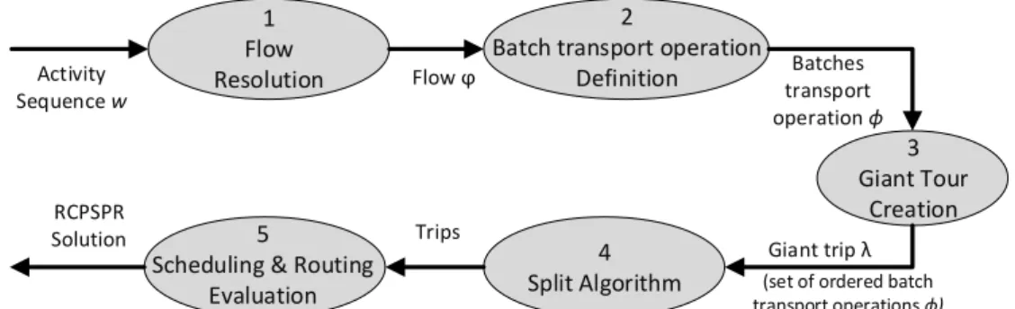
Contrary to classical approaches in scheduling or in routing (where a giant tour is transformed into trips thanks to only one function), the assignment of one solution to one activity sequence 𝑤 is a five-step procedure (Fig. 7) requiring successive resolutions of one flow problem, pre-calculation of the batch transport operation, generation of a giant tour and the splitting of the giant tour into trips with an evaluation to simultaneously address scheduling and routing constraints. After the evaluation procedure, a local search procedure can be applied to transform a solution of RCPSPR into a local minima.

Fig. 7. The evaluation procedure applied to obtain a RCPSPR solution

4.4. Flow definition (first step of the evaluation)

Because the problem cannot be efficiently divided into sub-problems considering the flow problem first and the routing second, there is no possibility of providing a quality flow solution since the criteria to optimize cannot be taken into account during the flow resolution. Nevertheless, it is possible to use time efficient approaches to provide flow solutions. In the next sections, numerical experiments prove that this assertion is relevant since the optimal flow solution (flow providing the minimal scheduling finishing time for the RCPSP) does not lead to the optimal RCPSPR one.

Activity schedules Solutions

Local search Evaluation 1 Flow Resolution 3 Giant Tour Creation 4 Split Algorithm Activity Sequence w Flow ϕ Batches transport operation ϕ Giant trip λ Trips RCPSPR Solution 2

Batch transport operation Definition

5

Scheduling & Routing

Because the solutions are encoded as a sequence of activities, the scheduling decision consists in defining the flow 𝜑𝑤(𝑖)𝑤(𝑗) (flow from node 𝑤(𝑖) to node 𝑤(𝑗); Fig 8) satisfying the activity resource requirement with the flow

transfer. The flow conservation at every node is required, except for dummy nodes 0 and n+1. The output graph 𝐺𝜑(𝑤) is the graph, with a flow 𝜑 satisfying the precedence constraints induced by the feasible sequence 𝑤. To

obtain an efficient computation time algorithm (avoiding a costly repair procedure), it is only possible to create an acyclic graph by the introduction of a constraint in the flow linked to the order of the sequence of activities (∀𝑗 < 𝑖, 𝜑𝑤(𝑖)𝑤(𝑗)= 0). Taking advantage of the special structure of the graph, it is possible to provide heuristic

resolution schemes offering a flow on a preferential basis to the closest activities.

Fig. 8. Constraints on flow

The first loop from step 11 to 21 (in Algorithm 1) iterates on the activities considering the remaining amount of resources available after the process of activity 𝑤(𝑖) i.e. 𝑏_𝑤(𝑖). The second loop scans all successive activities considering the maximal quantity of resources that can be transferred from 𝑤(𝑖) to 𝑤(𝑗). At each iteration, the remaining resources quantities 𝑟 and 𝑙 respectively for activities 𝑤(𝑖) and 𝑤(𝑗) are updated considering 𝑣 = 𝑚𝑖𝑛 (𝑟, 𝑙).

Procedure name: Flow Definition

1. procedure Flow_Definition 2. input parameters 3. 𝑤: activity sequence 5. output parameters 6. 𝜑: a flow 7. global parameter 8. n: number of activities 9. begin 10. i:=0 11. while (i < n) 12. if (i = 0) r = B else r = 𝑏_𝑤(𝑖) 13. stop = 0; j = i+1; 14. l := 𝑏_𝑗 15. while ((stop=0)and (j ≤ n)) 16. v := min(r, l) 17. r := r-v ; l := l-v 18. if (r = 0) stop = 1 else j := j + 1 19. endwhile 20. i := i + 1 21. endwhile 22. end

Algorithm 1. Flow Definition procedure

This greedy approach, applied to the sequence of activities 𝑤 = [0, 3, 2, 4 ,1, 5, 7 ,6 ,8 ,9] for a total amount of six units of resources available on node 0 (𝐵0= 6) provides the solution in Fig. 9.

Fig. 9. Example of flow solution

4.5. Batch transport operation definition (second step of the evaluation)

With the flow created in the previous steps, all the quantities that must be transferred between activities are defined. The flow 𝜑𝑖𝑗 created between activity 𝑖 and activity 𝑗 defines a batch flow transport operation with only one

transport operation (𝑖, 𝑗,∗, 𝜑𝑖𝑗) where 𝜑𝑖𝑗 could exceed the vehicle capacity and may require several transport

operations due to the vehicle capacity constraints (𝑐𝑣). For one batch flow transport operation, it is possible to

define different batch transport operations 𝜙𝑖𝑗 = ⋃ (𝑖, 𝑗,∗, 𝑘)𝑥 𝑥 / ∑𝑥𝑘𝑥=𝜑𝑖𝑗 with different properties. In other

0

w

i

j

ϕ

0

3

2

4

1

5

7

6

8

9

words, a batch transport operation 𝜙_𝑖𝑗 is an ordered set of transport operations from activity 𝑖 to 𝑗, and each transport operation (𝑖, 𝑗,∗, 𝑘) is fully defined by the quantity of resource to transport.

For example, a unitary batch transport operation 𝜙𝑖𝑗 = ⋃ (𝑖, 𝑗,∗ ,1)𝑥 𝑥 defines a set of transport operations that can

be assigned to any vehicle. For a non-unitary batch transport operation 𝜙𝑖𝑗= ⋃ (𝑖, 𝑗,∗, 𝑘)𝑥 𝑥, a transport operation

(𝑖, 𝑗,∗, 𝑘) can be assigned only to one vehicle 𝑢 of capacity 𝑐𝑢≥ 𝑘.

The definition of a batch transport operation (set of transport operations (𝑖, 𝑗,∗, 𝑘)) makes it possible to define a giant tour and to then create the trips with the split procedure. The quantity of resources in each transport operation (𝑖, 𝑗,∗, 𝑘) ∈ 𝜙𝑖𝑗 has an impact on the split execution since the split procedure is devoted to the aggregation of

transport operations (see Prins (2004)). Unprofitable batch transport operations can lead to a giant tour that does not permit investigation of all aggregations due to the vehicle capacity.

The key point is that several transport operations between 𝑖 and 𝑗 should be aggregated (in the split procedure) if they are consecutive in the giant tour. This aggregation creates a single transport operation from several transport operations (with the quantity of resources equal to the sum of the transport operations), avoiding both loaded and unloaded transport operations.

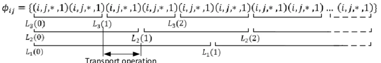
For example, a unitary batch transport operation 𝜙𝑖𝑗 = {(𝑖, 𝑗,∗ ,1)(𝑖, 𝑗,∗ ,1)(𝑖, 𝑗,∗ ,1)} can be aggregated in order to

obtain one batch transport operation 𝜙𝑖𝑗 = {(𝑖, 𝑗,∗ ,3)} composed of only one transport operation with three units

of resources. The aggregation is possible only if there is a vehicle that can transport such a quantity of resources. An issue can arise in some cases, for example, if a batch transport operation 𝜙𝑖𝑗 = {(𝑖, 𝑗,∗ ,2)(𝑖, 𝑗,∗ ,2)} is created

from a batch flow transport operation (𝑖, 𝑗,∗, 𝜑𝑖𝑗) with 𝜑𝑖𝑗= 4. In this example, the split will not be able to

aggregate the transport operation in order to obtain (𝑖, 𝑗,∗ ,3)(𝑖, 𝑗,∗ ,1), for example, which could be the best aggregation/assignment.

Unitary batch transport operation

The unitary batch transport operation makes it possible to create a number of transport operations (equal to the flow value) and to assign all transport operations of the batch to all vehicles.

For any pickup operation on activity 𝑖 and any delivery operation on activity 𝑗 with a flow 𝜑𝑖𝑗, the problem

consists in creating 𝜑𝑖𝑗 transport operations (𝑖, 𝑗,∗ ,1) to model all combinations of transport for all vehicles. This

batch of transport operations can be written with a set of unitary transport operations 𝜙𝑖𝑗 = {(𝑖, 𝑗,∗ ,1), … , (𝑖, 𝑗,∗

,1)} with 𝐶𝑎𝑟𝑑(𝜙𝑖𝑗) = 𝜑𝑖𝑗. With one unitary batch transport, the split procedure in the next step, can investigate

all possible aggregations without any additional constraints. In spite of this advantage, such a situation is also unprofitable, first, for the split procedure that investigates all aggregations of transport operations (and assignment to vehicles) and, second, for the giant tour length.

Key features for an efficient batch transport operation

To favor the split procedure used next in the framework, it is of particular interest to provide a batch of transport operations with minimal length (minimal number of transport operations), leading to the same aggregations of transport operations as the unitary batch transport operations. Let us note 𝜙_𝑖𝑗∗ = {(𝑖, 𝑗,∗, 𝜑₁) … (𝑖, 𝑗,∗, 𝜑_𝑚)} as the set of transport operation between 𝑖 and 𝑗 with the minimal number of transport operations.

Figure 10 illustrates an example composed of a heterogeneous fleet of three vehicles, with 𝑐1= 5, 𝑐2= 3, 𝑐3= 2

and a total amount of resources of 𝜑𝑖𝑗 = 12 to transport from 𝑖 to 𝑗.

Case 1

Case 1:

Let us consider a batch of transport operations where all transport operations are defined with two units of resources: 𝜙_𝑖𝑗 = {(𝑖, 𝑗,∗ ,2)(𝑖, 𝑗,∗ ,2)(𝑖, 𝑗,∗ ,2)(𝑖, 𝑗,∗ ,2)(𝑖, 𝑗,∗ ,2)(𝑖, 𝑗,∗ ,2)}.

Regardless of the vehicle (vehicle 2 or 3) used for 𝜙𝑖𝑗,

the number of transport operations is exactly equal to 6 since no aggregation can be achieved (Fig. 10 - case 1). i j D1 D2 P2 P1 2 2 D6 2 P6 i j D1 D2 P2 P1 D6 2 P6

=

Case 2

Case 3

Fig. 10. Batch transport operation constraints on split

with vehicles of capacity 2 and 3 (case 1 to 3)

Case 2:

If 𝜙_𝑖𝑗 is composed of transport operations with two or one units of resources, some transport operations can be aggregated. For example, with 𝜙𝑖𝑗 = {(𝑖, 𝑗,∗

,2)(𝑖, 𝑗,∗ ,1)(𝑖, 𝑗,∗ ,1)(𝑖, 𝑗,∗ ,2)(𝑖, 𝑗,∗ ,1)(𝑖, 𝑗,∗ ,1)(𝑖, 𝑗,∗ ,2)(𝑖, 𝑗,∗ ,1)(𝑖, 𝑗,∗ ,1)}, vehicle 3 requires six transport operations but vehicle 2 of capacity 3 can achieve only five transport operations, as illustrated in Fig. 10 (case 2).

Case 3:

A more promising set ϕij is defined by 𝜙𝑖𝑗=

{(𝑖, 𝑗,∗ ,2)(𝑖, 𝑗,∗ ,1), (𝑖, 𝑗,∗ ,1)(𝑖, 𝑗,∗ ,2)(𝑖, 𝑗,∗ ,2)(𝑖, 𝑗,∗ ,1)(𝑖, 𝑗,∗ ,1)(𝑖, 𝑗,∗ ,2)}, where vehicle 2 can achieve only four transport operations (Fig. 10 - case 3).

Figure 10 proves that for the same pickup/delivery operation(pickup operation on activity 𝑖 and delivery operation on activity 𝑗 and a flow 𝜑𝑖𝑗= 12), it is possible to define different batch transport operations 𝜙𝑖𝑗 (by defining the

quantity of resources of each transport operation), leading to a different number of transport operations due to different possible aggregations. For example, 𝜙_𝑖𝑗 = {(𝑖, 𝑗,∗ ,2)(𝑖, 𝑗,∗ ,1)(𝑖, 𝑗,∗ ,1)(𝑖, 𝑗,∗, )(𝑖, 𝑗,∗ ,2)(𝑖, 𝑗,∗ ,1)(𝑖, 𝑗,∗ ,1)(𝑖, 𝑗,∗ ,2)} (case 3 of Figure 10), composed of eight transport operations, can be aggregated for vehicle 3 to define only four transport operations.

In all the cases introduced in Fig. 10, the choice of 𝜙𝑖𝑗 does not impact the aggregation for vehicle 3, but case 3

for vehicle 2 is the most interesting case since it provides the minimal number of transport operations. Moreover, in case 3, 𝜙𝑖𝑗 is composed of eight transport operations, which is less than 12 transport operations for the unitary

batch transport operation. Another point can be highlighted by also taking vehicle 1 into account using case 3 (Fig. 11).

Fig. 11. Batch transport operation constraints on split with vehicles of capacity 2, 3 and 5

The problem of a batch transport definition must be addressed to create batch transport operations, with adapted solutions for all vehicles in the aggregation/assignment carried out in the split procedure.

Proposition for a batch transport definition

To create batch transport operations favoring the split procedure, the algorithm consists in investigating all cutoff points of all vehicles addressed separately with 𝐿𝑢, the ordered set of cutoff points of vehicle 𝑢. The set of cutoff

points of one vehicle is defined by the sum of flow of each transport operation. Let us denote 𝐿 = ⋃ 𝐿𝑢 𝑢 as the

ordered set of all cutoff points of all vehicles (without duplication).

For the first vehicle, the smallest batch transport operation is equal to 𝜙𝑖𝑗= {(𝑖, 𝑗,∗ ,5)(𝑖, 𝑗,∗ ,5)(𝑖, 𝑗,∗ ,2)}, defining

a set of cutoff points equal to 𝐿₁= (0, 5, 10,12). A similar remark holds for vehicle 2 considering 𝜙_𝑖𝑗= {(𝑖, 𝑗,∗ ,3)(𝑖, 𝑗,∗ ,3)(𝑖, 𝑗,∗ ,3)(𝑖, 𝑗,∗ ,3)} which leads to the following set of cutoff points: 𝐿2= (0, 3, 6, 9, 12). For

the third vehicle with 𝜙_𝑖𝑗 = {(𝑖, 𝑗,∗ ,2)(𝑖, 𝑗,∗ ,2)(𝑖, 𝑗,∗ ,2)(𝑖, 𝑗,∗ ,2)(𝑖, 𝑗,∗ ,2)(𝑖, 𝑗,∗ ,2)}, the set of cutoff points is: 𝐿3= (0, 2, 4, 6, 8, 10, 12. ). For this example, 𝐿 = (0,2,3,4,5,6,8,9,10,12).

i j D1 D2 P2 P1 2 2 D6 2 P6 i j D1 D2 P2 P1 1

≠

≠

≠

≠

Next, the transport operations of the unitary batch transport operation are iteratively scanned and gathered into a new transport operation (𝑖, 𝑗,∗, 𝜑𝑖𝑗). These transport operations are defined between two successive cutoff points

of 𝐿 and define 𝜙𝑖𝑗.

Fig. 12. Representation of the cutoff point on the unitary batch transport operation for the example with three

vehicles, 𝑐1= 5, 𝑐2= 3, 𝑐3= 2 and a total amount of resources of 𝜑𝑖𝑗 = 12

The best batch transport operation is built according to all the cutoff points. In this example, the best batch transport operation according to this definition is equal to:

𝜙𝑖𝑗∗ = {(𝑖, 𝑗,∗ ,2)(𝑖, 𝑗,∗ ,1)(𝑖, 𝑗,∗ ,1)(𝑖, 𝑗,∗ ,1)(𝑖, 𝑗,∗ ,1)(𝑖, 𝑗,∗ ,1)(𝑖, 𝑗,∗ ,2)(𝑖, 𝑗,∗ ,1)(𝑖, 𝑗,∗ ,1)(𝑖, 𝑗,∗ ,1)}.

4.6. Giant tour construction (third step of the evaluation)

The giant tour construction consists in scanning the set of batch flow transport operations with only one transport operation (𝑤(𝑖) , 𝑤(𝑗) ,∗, 𝜑𝑤(𝑖)𝑤(𝑗)) in the increasing order of 𝑤(𝑖) and 𝑤(𝑗) and to schedule the batch

transport operation 𝜙𝑤(𝑖)𝑤(𝑗) at the best possible location. The HGT procedure (Heuristic for Giant Tour) defines

a depth-first-search strategy by a greedy insertion of each batch transport operation 𝜙𝑖𝑗 at the best possible position.

Let us note that the heuristic does not schedule transport operations one-by-one but, instead, the batch transport operations with all the transport operations that compose it. The construction is based on a best_insertion (𝜆, 𝑐𝑜𝑠𝑡) procedure that finds the best insertion position of the last scheduled batch transport operation with respect to the precedence and the resource constraints, calculating the minimal insertion cost equal to the empty transport between the last scheduled batch transport operation and the transport operation on the right of the insertion position.

Example:

Let us consider 𝑤 = [0, 3, 2, 4 ,1, 5, 7 ,6 ,8 ,9] and the flow solution of Fig. 9. To build a giant tour, each batch transport operation associated with one flow is inserted at the best position. Some of the steps are detailed in Table 1.

Table 1

Steps to build a giant tour

Batch to insert

Possible Giant Tours 𝜆 Cost Best Step 1: 𝜙={(0,3,*,2)} (0,3,*,2) -  Step 2: 𝜙={(0,2,*,2)} (0,3,*,2)(0,2,*,2) 3  (0,2,*,2)(0,3,*,2) 4 Step 3: 𝜙={(0,4,*,2)} (0,3,*,2)(0,2,*,2)(0,4,*,2) 4  (0,3,*,2)(0,4,*,2)(0,2,*,2) 10 (0,4,*,2)(0,3,*,2)(0,2,*,2) 10 Step 4: 𝜙={(3,1,*,2)} (0,3,*,2)(0,2,*,2)(0,4,*,2)(3,1,*,2) 13 (0,3,*,2)(0,2,*,2)(3,1,*,2)(0,4,*,2) 3  (0,3,*,2)(3,1,*,2)(0,2,*,2)(0,4,*,2) 3 … Step 14: 𝜙={(8,9,*,2),(8,9,*,1)} (0,3,*,*,2)(0,2,*,*,2)(3,1,*,*,2)(0,4,*,2)(4,5,*,2) (5,6,*,2)(4,5,*,2)(5,8,*,1)(1,7,*,2)(7,8,*,2)(6,9,*,2) (7,9,*,1)(8,9,*,2)(8,9,*,1) 3  (0,3,*,2)(0,2,*,2)(3,1,*,2)(0,4,*,2)(4,5,*,2)(5,6,*,2) (4,5,*,2)(5,8,*,1)(1,7,*,2)(7,8,*,2)(6,9,*,2)(8,9,*,2) (8,9,*,1)(7,9,*,1) 4 (0,3,*,2)(0,2,*,2)(3,1,*,2)(0,4,*,2)(4,5,*,2)(5,6,*,2) (4,5,*,2)(5,8,*,1)(1,7,*,2)(7,8,*,2)(8,9,*,2) (8,9,*,1)(6,9,*,2)(7,9,*,1) 6 Transport operation

In Step 4, the batch transport operation 𝜙 = {(3,1,∗ ,2)}can be located on three positions but cannot be inserted at the first place of the sequence. The first transport operation (0,3,∗ ,2) defines a pickup of two units of flow at activity 0 and a delivery of two units at activity 3. Consequently, the transport (3,1,∗ ,2) cannot be scheduled before (0, 3,∗ ,2) since (3,1,∗ ,2) defines a pickup at activity 3, which obviously required a previous delivery at activity 3.

In Step 14, the batch transport operation is composed of two transport operations that can be inserted on three positions, and the best insertion is located at the end of the giant tour.

4.7. Split algorithm (fourth step of the evaluation)

The split procedure, taken from routing, tackles only constraints taken from routing, including a limited number of vehicles, a limitation on hub capacity (see Duhamel et al. (2012) for a generic definition of split procedures). The main difference in the new split consists of the management of both the availability of vehicles and of activities. As highlighted in Duhamel et al. (2012), a label saved on a node models a state of the dynamic algorithm and must be defined by a cost and a full description of the system state. A split-based approach must tackle the following features:

 A label definition to model the system state;  A propagation rule to create new labels;

 A dominance rule to save only non-dominated labels on the node.

A special feature of the split, dedicated to the RCPSPR, is the fact that the system state encompasses both the vehicle fleet state and the activity state:

 The vehicle fleet state is composed of three pieces of information for each vehicle: the position of the vehicle, the departure time and the arrival time. These data are required even if the fleet is homogeneous.

 The activity state is given by the earliest starting time of all the activities.

At each step of the split algorithm, the current system state is composed of the activity that has been scheduled but not achieved (see, for example, activity 5 in Fig. 13), activities previously scheduled, and vehicles at some specific location corresponding to their last loaded transport. Before achieving one transport operation (𝑖, 𝑗, 𝑢, 𝜑), the vehicle 𝑢 has to be available and located on activity 𝑖, which may involve an unloaded transport. The cost of this unloaded transport depends of the current localization of the vehicle.

The split procedure consists of building an auxiliary acyclic graph 𝐻 with 𝑛𝑡 + 1 nodes numbered from 0 to 𝑛𝑡 (𝑛𝑡 is the number of transport operations in the giant tour 𝜆) where an arc from node 𝑖 to 𝑗 represents a subsequent 𝜇𝑖𝑗 of transport operations from the giant tour with 𝜇𝑖𝑗= (𝜆(𝑖 + 1),…, 𝜆(𝑗)), where 𝜆(𝑖) is a transport operation.

For the sake of convenience, 𝜆+_{(𝑖) denotes the pickup operation of 𝜆(𝑖), 𝜆}−_{(𝑖) the delivery operation of 𝜆(𝑖), and}

𝜆𝜑_{(𝑖) the flow associated with the transport operation 𝜆(𝑖).}

Fig. 13. System state during the Split at step 𝑖

The optimal splitting of 𝜆 (or quasi-optimal splitting in the event of extra constraints concerning the use of resources) corresponds to a min-cost path from node 0 to 𝑛𝑡 node in 𝐻. It can be computed using a Bellman-like algorithm taking the vehicle fleet into account, i.e., several labels have to be tackled per node. The principle is

1 2 3 4 5 6 7 8 9 20 30 40 50 60 70 80 90 100

Transport operation (load) Transport operation (unload) Activities Time S=3, C=23 S=10, C=25 S=10, C=40 S=27, C=37 S=53, C=63 S’=66, C’=96 S’=96, C’=106 10 0 0

Activity waiting time Vehicle waiting time S’=34, C’=64

endorsed by defining labels that model the current state of the global system, a propagation rule and a dominance between labels.

Label definition

To extract the vehicle trips from the giant tour, a set of non-dominated labels is stored on each node of the graph 𝐻. A label represents a partial solution evaluation that tackles tasks 𝜆(0) to 𝜆(𝑗). Let us denote 𝐿𝑗_𝑖 the 𝑖𝑡ℎ

label on node 𝑗, which is composed of a 3𝑣-tuple 𝑉_𝑖𝑗, a 𝑛 + 1-tuple 𝑆_𝑖𝑗 and of a couple (𝑓𝑢, 𝑓𝑣):

 A 3𝑣-tuple 𝑉_𝑖𝑗 _{defining both vehicle times and position, 𝑉}

𝑖𝑗= (𝐵𝑖𝑗1, … , 𝐵𝑖𝑗𝑣, 𝐴1𝑖𝑗, … , 𝐴𝑖𝑗𝑣, 𝑃𝑖𝑗1, … , 𝑃𝑖𝑗𝑣) where

𝑃𝑖𝑗1, … , 𝑃𝑖𝑗 𝑣 are the current position of each vehicle (𝑃𝑖𝑗𝑢= 𝑝 means that the position of the vehicle 𝑢 is on

activity 𝑝), 𝐵𝑖𝑗1, … , 𝐵𝑖𝑗𝑣 give the earliest departure time of the vehicles, and 𝐴1𝑖𝑗, … , 𝐴𝑖𝑗𝑣 are the arrival time of

the vehicles.

 An 𝑛 + 1-tuple 𝑆_𝑖𝑗 _{defining the earliest starting time of each activity 𝑆}

𝑖𝑗 = ( 𝑆𝑖𝑗 0, … , 𝑆𝑖𝑗𝑛+1);

 A couple (𝑓𝑢, 𝑓𝑣) of positions referring to the father label of 𝐿𝑗𝑖 𝑖. 𝑒. 𝐿𝑖𝑗 that has been generated using the label

number 𝑓𝑢 on node number 𝑓𝑣.

Label propagation

A propagation function defined by 𝑓: L  T → R permits the generation of a new label 𝐿𝑞𝑗 from one label 𝐿𝑖𝑝 and a

trip evaluation 𝛾 depending of the subsequence 𝜇𝑖𝑗 with a cost equal to transportation time from 𝜆+(𝑗) to 𝜆−(𝑗), i.e.,

𝑡𝜆+_(𝑗),𝜆−_(𝑗).For a subsequent 𝜇_𝑖𝑗= (𝜆(𝑖 + 1), … , 𝜆(𝑗)), the new label 𝐿_𝑞𝑗 for node 𝑗 is defined from the label 𝐿𝑖𝑝 considering the next update, using vehicle 𝑢:

𝐵𝑞𝑗𝑢 = max(𝑆𝑝𝑖 𝜆+_(𝑗) + 𝑝𝜆+(𝑗); 𝐵𝑝𝑖𝑢 + 𝑒𝑃_𝑝𝑖𝑢,𝜆+(𝑗)) 𝐵𝑞𝑗𝑣 = max(𝐵𝑝𝑖𝑣; 𝐴𝑣𝑝𝑖) / 𝑣 ≠ 𝑢 𝐴𝑞𝑗𝑢 = 𝐵𝑞𝑗𝑢 + 𝑡𝜆+(𝑗),𝜆−_(𝑗) 𝑃𝑞𝑗𝑢 = 𝜆−(𝑗) 𝑆_𝑞𝑗𝜆−(𝑗)= max(𝑆_𝑝𝑖𝜆−(𝑗); 𝐴𝑞𝑗𝑢)

For the label 𝐿𝑖𝑝, all assignments to vehicles are investigated, leading to 𝑣 labels. These final labels are included or

not depending on the set of non-dominated labels previously stored on the node 𝑗. Dominance rule

To keep only non-dominated labels on nodes, a dominance rule must be defined. Considering two labels 𝐿𝑖𝑝 and 𝑃,

𝐿𝑖𝑝 is defined as dominant as regards 𝐿𝑖𝑞 ( 𝐿𝑖𝑞≪ 𝐿𝑖𝑝) if the following two conditions hold:

Condition 1. All vehicles have the same location: ∀𝑢 ∈ 𝑇, 𝑃_𝑖𝑝𝑢 = 𝑃_𝑖𝑞𝑢 Condition 2. ∀𝑢 ∈ 𝑇, 𝐴𝑢_𝑖𝑝≤ 𝐴_𝑖𝑞𝑢 and ∃𝑢 ∈ 𝑇, 𝐴_𝑖𝑝𝑢 < 𝐴_𝑖𝑞𝑢

Let us note that the earliest starting time of activities is not relevant for the dominance rule since if all vehicle time availabilities of label 𝐿𝑖𝑝 are less than or equal to vehicle availabilities on the label, then 𝐿𝑖𝑞, ∄𝑘/ 𝑆𝑖𝑞𝑘 < 𝑆𝑖𝑝𝑘 .

Labels stored on nodes

If 𝐿𝑖𝑝 is not dominant with regard to 𝐿𝑖𝑞 ( 𝐿𝑖𝑞 ≪̅ 𝐿𝑖𝑝), this does not imply that 𝐿𝑖𝑞 is dominant with regard to 𝐿𝑖𝑝. If

𝐿𝑖𝑞≪̅ 𝐿𝑖𝑝 and 𝐿𝑝𝑖 ≪̅ 𝐿𝑖𝑞, then 𝐿𝑖𝑝 cannot be compared to 𝐿𝑞𝑖. Thus, if ∃𝑘 on node 𝑖/ 𝐿𝑖𝑝≪ 𝐿𝑖𝑘, then 𝐿𝑝𝑖 is not

added to node 𝑖.

On the other hand, each label 𝐿𝑘𝑖/ 𝐿𝑖𝑘 ≪ 𝐿𝑖𝑝 can be removed from node 𝑖. The dominance rule limits the number

of labels stored at each node to a minor subset while maintaining split optimality. An additional time-saving approach consists in limiting the maximal number 𝑁𝐿 of labels generated during the split process or per node. Such

restrictions, in addition to the dominance rule, can strongly reduce the CPU time, but can yield a sub-optimal splitting solution with no real drawback on the global solution found at the end of the split, as reported by Boudia et al. (2007).

Figure 14 gives some steps of the split procedure applied on the giant tour of the example detailed in Table 1. The initial label on node 0 is ((0,0,0,0,0,0)(0,0,0,0,0,0,0,0,0,0)) and it is propagated on the auxiliary graph with the arc between node 0 and 1 corresponding to the transport operation (0,3,∗ ,2) using the two possible vehicles. For

example, the transport operation can be carried out by vehicle 1 available at activity 0 on time 0. The duration of this transport operation is equal to 3, the propagation rule updates the arrival time of the vehicle to 3, the position is also equal to 3, and the earliest starting time of activity 3 has a value of 3. This process is iterated to obtain a set of eight labels on node 3 where each label represents a specific partial solution (see Fig. 14). With the dominance rule, only six of these eight labels are saved and the two underlined labels are deleted.

Fig. 14. Example of labels generated by the split in the auxiliary graph (data available at:

http://fc.isima.fr/~vinot/Research/RCPSP&Routing.html)

Procedure name: Split

1. procedure Split 2. input parameters 3. 𝜆: giant tour

4. k: number of transport operation in the giant tour 5. output parameters

6. S: Solution graph 7. global parameter

8. n: number of activities 9. v: number of vehicles

10. NL: maximum number of labels on each node 11. begin

12. call InitGraph(S, 𝜆, k, n, v, NL) 13. i:=0

14. while (i < k)

15. j := i+1; flow := 0

16. while (CompareTransportOperation(𝜆, i+1, j)=1) 17. flow := flow + 𝜆𝜑_(𝑗)

18. for k := 1 to NBi do //for each label on node i

19. n_vehicle := 1

20. while ((n_vehicle ≤ v) and (flow ≤ cn_vehicle)) then 21. P := call PropagateLabel(𝜆(𝑗), flow, n_vehicle, 𝐿𝑖𝑘) 22. if (NBj = 0) then call InsertLabel(P, j, S, NL) 23. else insert:=0

24. insert := call TestInsertLabel(P, j, S)

25. if (insert=1) then call InsertLabel(P, j, S, NL) endif 26. endif 27. n_vehicle := n_vehicle + 1 28. endwhile 29. endfor 30. j := j + 1 31. endwhile 32. i := i + 1 33. endwhile

34. S := call Extract_trips () //save the best solution 35. end

Algorithm 2. Split procedure

The split is detailed in Algorithm 2 and uses low-level procedures to handle the labels:  InitGraph(S,𝜆,k,n,v,NL) initializes all the local variables of the solution;

 CompareTransportOperation(λ,i,j): the function returns 1 if the transport operation 𝜆(𝑖 + 1) and 𝜆(𝑗) have the same pickup and delivery operations, i.e., 𝜆−_{(𝑖 + 1) = 𝜆}−_{(𝑗) and 𝜆}+_{(𝑖 + 1) = 𝜆}+_(𝑗);

 PropagateLabel(𝑇(𝑖,𝑗,𝑢,𝑥) ,flow,v,L)uses the propagation rule to generate the label P from 𝐿, knowing the

transport operation 𝑇(𝑖,𝑗,𝑢,𝑥) , the flow and the vehicle 𝑣 used;

0 Transport operation 1 Transport operation 2 ((0,0,0,0,0,0),(0,0,0,0,0,0,0,0,0,0)) (0,3,*,2) (0,2,*,2) V1 V2 V1 3 V2 Transport operation (3,1,*,2) V1 V2 ((0,0,3,0,3,0),(0,0,0,3,0,..,0)) ((0,0,0,3,0,3),(0,0,0,3,0,..,0)) V1 V2 ((6,0,10,0,2,0),(0,0,10,3,0,..,0)) V1 V2 V1 V2 V1 V2 ((23,0,27,0,1,0),(0,27,10,3,0,..,0)) ((10,23,10,27,2,1),(0,27,10,3,0,..,0)) ((23, 4,27,4,1,2),(0,27,4,3,0,..,0)) ((3,23,3,27,3,1),(0,27,4,3,0,..,0)) ((3,0,3,4,3,2),(0,0,4,3,0,..,0)) ((0,3,4,3,2,3),(0,0,4,3,0,..,0)) ((0,6,0,10,0,2),(0,0,10,3,0,..,0)) ((4,23,4,27,2,1),(0,27,4,3,0,..,0)) ((23,3,27,3,1,3),(0,27,4,3,0,..,0)) ((0,23,0,27,0,1),(0,27,10,3,0,..,0)) ((23,10,27,10,1,2),(0,27,10,3,0,..,0))

 TestInsertLabel(P,j,S) compares the label 𝑃 to the labels on node 𝑗. If the label 𝑃 dominates at least one label, the procedure returns 1 and the label dominated is deleted; otherwise, the procedure returns 0;  InsertLabel(P,j,S,NL) inserts the label 𝑃 on node 𝑗 in ascending order of the maximal value of the vehicle

time availability. The number of labels on node 𝑗 cannot exceed 𝑁𝐿;

 Extract_trips() validates the best final label and returns the solution with the set of trips.

The split algorithm (Algorithm 2) is composed of two parts: the initialization part where local variables are initialized (line 12) and a loop from lines 14 to 33 that iterates for the ordered set of customers defined by the giant tour 𝜆. The second loop from lines 16 to 31 iterates and makes it possible to evaluate the partial sequence (λ(i + 1), … , λ(j)) on each label on node 𝑖 with the loop from lines 18 to 29.

The third loop (from lines 20 to 28) iterates and makes it possible to calculate the partial sequence (λ(i + 1), … , λ(j)) using each vehicle with a sufficient capacity, leading to a label 𝑃 (line 21), which is then inserted into the list of labels on node 𝑗, using the InsertLabel procedure. The best solution is saved at the end of the algorithm (line 34).

4.8. Scheduling and routing evaluation (fifth step of the evaluation)

The fully oriented disjunctive graph that models a solution is obtained, including both activity disjunctions and transport disjunctions and is then evaluated with a longest path algorithm to provide a semi-active solution.

4.9. Local search

Random initial solutions are obtained by random definition of activity sequence 𝑤 limited to the space of non-level decreasing activity lists. In order to remove such restriction, neighborhoods can be obtained by the 𝑆𝑤𝑎𝑝(𝑢, 𝑣) operator, leading to a feasible move if there is no edge modeling a precedence constraint at indices 𝑢 + 1 to 𝑣. The whole space of the feasible activity sequence can be investigated.

To improve a RCPSPR solution, an efficient local search algorithm can be defined considering the critical path (Fig. 15 provides a graphical solution of the shortest path linked to the example of Fig. 10) with the introduction of blocks whose classification extends the scheduling blocks commonly used (Laarhoven et al., 1992; Matsuo et al., 1988; Dell'amico and Trubian, 1993; Nowicki and Smutnicki, 1996):

Block type 1: a transport operation and an activity; Block type 2: two transport operations;

Block type 3: an activity and a transport operation; Block type 4: two activities.

The local search investigates moves from the end of the critical path to the starting node and, depending on the block type encountered among the critical path, the actions are investigated on the activity sequence 𝑤 only, thanks to the indirect representation of solutions. If one action leads to a lower cost solution, the critical path exploration is restarted at the end of the graph.

Block type 1 models a situation where the activity starting time depends on the transport operation (𝑖, 𝑗, 𝑢, 𝜑), which transports 𝜑 units of resource required by activity 𝑗. To obtain a neighborhood solution where this situation does not occur, the transport operation between the two activities must not be required. It can be obtained by a left shifting of the activity 𝑗 into the activity sequence 𝑤 to the left of activity 𝑖.

Fig. 15. Example of a critical path

0 3 5 8 6 9 0 20 10 10 2 3 1 1 3 1 1 3 1 3 0 0 3 109 106 66 96 63 53 50 30 23 17+3=20 4+3=7 30 Block type 1 Block type 2 Block type 4 Block type 3

Block type 2 concerns two consecutive transport operations (𝑖, 𝑗, 𝑢, 𝜑) and (𝑘, 𝑝, 𝑣, 𝜑′), including an unloaded transport operation. In this situation, the second transport operation (𝑘, 𝑝, 𝑣, 𝜑′_{) has to wait to start for the end of}

the loaded transport operation (𝑖, 𝑗, 𝑢, 𝜑) and the end of the unloaded transport operations from 𝑗 to 𝑘. It can be achieved by a left shifting of activity 𝑘 to activity 𝑖.

Block type 3 models a situation that is quite identical to the situation of block type 1 and a similar approach holds. Block type 4 between two activities occurs when an activity waits until the end of another activity to start, which is necessary due to a precedence constraint between them. To try to delete this arc from the critical path, the first activity has to be scheduled earlier. It can be achieved by a shifting of the activity in the activity sequence 𝑤 with respect to the precedence constraint.

5

Numerical experiments

To the best of our knowledge, no instances dealing with this problem are available. Therefore, numerical experiments are based on the two sets of instances introduced below:

 The first one consists of the definition of a new set of small-scale instances with less than eight activities for which optimal resolution using CPLEX remains possible;

 The second one consists of the definition of medium-scale instances for about 30 activities not tractable by exact algorithms.

To favor fair future comparative studies, theses sets of instances are available at the following web page:

http://fc.isima.fr/~vinot/Research/RCPSP&Routing.html The numerical experiments are carried out to meet the following requirements:

 To prove (using the small-scale instances) that the sequential resolution of the two sub-problems (the flow problem and then the routing/scheduling) leads to suboptimal solutions;

 To evaluate the performance of the approach by a careful comparison of the optimal solutions provided by CPLEX with a MILP and the solutions provided by the GRASP×ELS;

 To evaluate the GRASP×ELS convergence on medium-scale instances for future researchers.

The linear formulation used by CPLEX is provided in the appendix and additional numerical experiments have been achieved using a Constraint Programming model with IBM ILOG CPLEX Optimization Studio (the model is also provided in the appendix)

For each instance, five replications of the GRASP×ELS have been carried out. For the sake of convenience, all experiments are carried out with the same set of parameters introduced in Table 2 and the following notations are used for all of the results:

 Avg denotes an average value

 LB lower bound values (equal to the optimal solution of a RCPSP with transfer times)  𝐿𝐵(𝑛𝑡𝑜𝑡) the minimal number of operations to be scheduled

 UB upper bound values  BFS best solution found

 TT total CPU time in seconds to execute the algorithm (end of the iterations for the GRASP×ELS and time to close the gap for CPLEX)

 T* CPU time in seconds to obtain the BFS

 Nb. Opt Number of instances where the solution has the same value as the lower bound

Table 2

Parameters setting

Parameter Definition Value

np Number of GRASP iterations 100

ne Number of ELS iterations 25

nd Number of neighborhood iterations 10

l Number of local research iterations 10

NBmax Maximum number of labels per node 20

All experiments are carried out on a single thread C program, using Visual Studio and Windows 7 as the operating system on a Dell Optiflex9020 with an Intel Core i7-4770 CPU 3.4 GHz and 16 Gb of RAM, which can be established at 2671 Mflops (see Dongarra et al. (2014)). The same set of parameters is used for all instances whatever the number of vehicles.