HAL Id: hal-00199381
https://hal.archives-ouvertes.fr/hal-00199381
Submitted on 18 Dec 2007
HAL is a multi-disciplinary open access
archive for the deposit and dissemination of
sci-entific research documents, whether they are
pub-lished or not. The documents may come from
teaching and research institutions in France or
abroad, or from public or private research centers.
L’archive ouverte pluridisciplinaire HAL, est
destinée au dépôt et à la diffusion de documents
scientifiques de niveau recherche, publiés ou non,
émanant des établissements d’enseignement et de
recherche français ou étrangers, des laboratoires
publics ou privés.
From pictures to extended finite elements: extended
digital image correlation (X-DIC)
Julien Réthoré, Stéphane Roux, François Hild
To cite this version:
Julien Réthoré, Stéphane Roux, François Hild. From pictures to extended finite elements: extended
digital image correlation (X-DIC). Comptes Rendus Mécanique, Elsevier Masson, 2007, 335,
pp.131-137. �10.1016/j.crme.2007.02.003�. �hal-00199381�
From pictures to extended finite elements:
Extended digital image correlation (X-DIC)
Corr´elation d’images num´eriques ´etendue (CIN´
E)
Julien R´
ethor´
e
aSt´
ephane Roux
bFran¸cois Hild
aa
LMT-Cachan, ENS de Cachan / CNRS UMR 8535 / Universit´e Paris 6 61 Avenue du Pr´esident Wilson, F-94235 Cachan Cedex, France
b
Surface du Verre et Interfaces, UMR CNRS/Saint-Gobain, 39 Quai Lucien Lefranc, 93303 Aubervilliers Cedex, France
Abstract
An image correlation algorithm accounting for discontinuities is proposed. It is based on a decomposition of the displacement field onto a regular finite element basis supported by a uniform mesh, enriched with suitable functions to describe accurately discontinuities, paralleling recent developments of extended finite elements. This algorithm is applied to a bolted assembly where interface slip is observed upon loading.
R´esum´e
Un algorithme de corr´elation d’images num´eriques capable de rendre compte de discontinuit´es est introduit. Il est fond´e sur une d´ecomposition du champ de d´eplacement sur une base r´eguli`ere de type ´el´ements finis support´es par un maillage homog`ene, enrichie par des fonctions de base adapt´ees aux discontinuit´es, suivant les d´eveloppements r´ecents des ´el´ements finis ´etendus. Cet algorithme est appliqu´e `a l’´etude d’un assemblage boulonn´e o`u un glissement est mobilis´e sous charge.
Key words: Rupture ; Discontinuity ; Photomechanics Mots-cl´es : Rupture ; Discontinuit´e ; Photom´ecanique
Email addresses: [email protected] (Julien R´ethor´e), [email protected] (St´ephane Roux), [email protected](Fran¸cois Hild).
Version fran¸caise abr´eg´ee
Les m´ethodes de mesure de champ sont particuli`erement attractives lorsque l’on souhaite analyser des ph´enom`enes localis´es (e.g., discontinuit´es faibles ou fortes). Parmi celles-ci, la corr´elation d’images num´e-riques est une des techniques optiques [1] des plus adapt´ees. Ainsi, par exemple, une approche int´egr´ee
a ´et´e d´evelopp´ee pour la mesure du facteur d’intensit´e des contraintes [2] pour des mat´eriaux `a
com-portement ´elastique-fragile. Les d´eplacements mesur´es peuvent ´egalement ˆetre utilis´es lors de simulations num´eriques `a titre de comparaison, ou mˆeme comme conditions aux limites impos´ees. Dans les deux cas, la coh´erence entre les hypoth`eses cin´ematiques faites lors de la mesure et de la simulation rendent les com-paraisons plus robustes. R´ecemment, la m´ethode des ´el´ements finis ´etendus (ELFE) a ´et´e introduite pour analyser des cin´ematiques discontinues sans remaillage [3]. Cette propri´et´e est particuli`erement s´eduisante lorsque des algorithmes de corr´elation sont d´evelopp´es car les incertitudes de mesure sont d’autant plus grandes que la taille des ´el´ements est petite [4].
L’objet de cette Note est de montrer qu’une cin´ematique enrichie peut ˆetre naturellement int´egr´ee dans un algorithme de corr´elation. Cette technique sera appel´ee “corr´elation d’images num´eriques ´etendue”. La d´emarche g´en´erale d’un algorithme de corr´elation, rappel´ee au paragraphe 1.1, permet de consid´erer une large vari´et´e de champs de d´eplacement. Dans sa version lin´earis´ee (3), la conservation du flot optique conduit `a la r´esolution d’un syst`eme lin´eaire (5) pour d´eterminer les composantes inconnues associ´ees `a la base cin´ematique choisie. Cette derni`ere est peu contrainte dans la formulation g´en´erale du probl`eme, la d´eclinaison particuli`ere d´evelopp´ee ici utilise une base d’´el´ements finis classique (polynomiale d’ordre un sur un support carr´e ou Q4P1). La d´ecomposition enrichie (10), adapt´ee aux ´el´ements finis ´etendus, est ensuite rappel´ee. Elle est impl´ement´ee dans une version (X-Q4), qui, dans cette Note, n’est illustr´ee que pour des discontinuit´es fortes lorsque la r´egion d’´etude est enti`erement travers´ee par celles-ci (Figure 1). L’exemple analys´e concerne un assemblage boulonn´e de trois plaques en alliage d’aluminium (Figure 2-a). Une analyse d’incertitude montre que l’enrichissement ne d´egrade pas significativement celle-ci lorsque des d´eplacements constants sont appliqu´es (Figure 3-a). Par contre, lorsque les d´eplacements appliqu´es sont discontinus, le gain est significatif avec la version ´etendue, bien que, dans l’exemple particulier ´etudi´e, le mouchetis ne soit pas optimal (Figure 3-b). L’analyse des deux discontinuit´es, l’une avec un champ enrichi et l’autre sans, montre l’int´erˆet (Figure 2) en termes d’amplitude de r´esidus et de leur localisation. De plus, une sensibilit´e assez faible de la version X-Q4 `a la taille de l’´el´ement est observ´ee (Figure 4).
L’algorithme discut´e ici a ´et´e particularis´e au cas o`u la discontinuit´e traverse toute la r´egion d’´etude. Il
peut ˆetre g´en´eralis´e [au sens de l’´equation (10)] au cas d’une surface fissur´ee voire `a celui de discontinuit´es faibles. Dans le cas pr´esent´e ici, la ligne de discontinuit´e a ´et´e (ais´ement) positionn´ee par l’utilisateur. A terme, une d´etection automatique sera impl´ement´ee.
Full-field measurements are useful when localized phenomena (i.e., weak or strong discontinuities) are observed. Digital image correlation is one of the optical techniques [1] that are used to capture these effects. For instance, an integrated approach was developed to measure stress intensity factors in elastic-brittle materials [2]. The measured displacement may be used in numerical simulations to compare both data, or even to prescribe measured quantities. In both cases, the fact that the kinematic hypotheses are kept identical allows one to be fully consistent from the experimental side (e.g., when pictures are analyzed) to the numerical one. Recently, the extended finite element method (X-FEM) was introduced to analyze discontinuous displacements without remeshing [3]. This particular feature is appealing when measurements are needed since the corresponding uncertainties increase as the element size decreases [4]. The aim of the Note is to show that the kinematics used in the extended finite element method may be used in a correlation algorithm. It corresponds to an extension of the DIC approach presented in Ref.
[4] when enriched functions are added to the basis of displacement fields. It is referred to as “eXtended Digital Image Correlation” (X-DIC).
1. Digital image correlation 1.1. General principle
Let us consider two digital (gray level) pictures shot at two different instants of time. The reference,
f, and the deformed state, g, pictures of a surface (represented here as gray level valued function of the
pixel coordinates) are related by the advection of the texture in the displacement field u
g(x) = f (x + u(x)) (1)
From the knowledge of f and g, the problem consists in estimating u as accurately as possible. The conservation of the optical flow (1) is linearized by assuming that the reference image is differentiable
Φ2
(x) = [u(x).∇f (x) + f (x) − g(x)]2
(2) and consists in minimizing the local residual Φ. To estimate u, the quadratic difference (right hand side of Eq. (2)) is integrated over the studied domain Ω and subsequently minimized
η2=
Z
Ω
[u(x).∇f (x) + f (x) − g(x)]2dx (3)
As such, the measurement of the displacement is an ill-posed problem. The point-wise displacement is only measurable along the direction of the intensity gradient, and thus calls for a regularization. The
displacement field is decomposed over a set of functions Ψn(x). In particular, each component of the
displacement field may be treated in a similar manner, and thus only scalar functions ψn(x) are introduced
u(x) =X
α, n
aαnψn(x)eα (4)
where eαare elementary unit vectors along each space dimension α and aαnthe corresponding amplitudes.
The objective function is thus a quadratic form of the unknowns aαn. Its minimization leads to a linear
system
Ma= b (5)
where ∂αf = ∇f.eα denotes the directional derivative, the matrix M and the vector b read
Mαnβm= Z Ω [ψm(x)ψn(x)∂αf(x)∂βf(x)]dx (6) and bαn= Z Ω [g(x) − f (x)] ψn(x)∂αf(x)dx (7)
When the functions ψn(x) are shape functions of finite elements, the proposed framework allows one to
develop a correlation algorithm that is in direct link with finite element simulations. In the following, it is proposed to discuss a technique to deal with strong discontinuities.
1.2. Extended digital image correlation
When discontinuous fields are sought, the previous framework is used with an enriched kinematics. If classical finite element shape functions were used, the discontinuity would be smoothed. One of the consequences may be a bias in the subsequent analysis of the displacement fields (e.g., evaluation of a stress intensity factor). The property of the partition of unity [5] of finite element shape functions over the zone covered by the set of nodes N
X
n∈N
Nn(x) = 1 (8)
is exploited to enrich the kinematic basis, where Nn are scalar shape functions to interpolate the
dis-placement u(x) in an element. The enriched discretization reads
u(x) = X n∈N , α aαnNn(x)eα+ X n∈Nenr, α dαnNn(x)ϕ(x)eα (9)
where ϕ is the enrichment function and Nenr is a sub-set of N in which nodes hold enriched degrees
of freedom dαn. The enrichment function can be chosen arbitrarily to capture a specific feature of the
displacement field in the minimization problem. In the following, we focus on displacement fields with strong discontinuities (e.g., cracks). For instance, the components of the displacement have a discontinuity across the crack front and a square root dependence close to the crack tip. In the original X-FEM, five enriched functions are used, namely one that is discontinuous across the crack front, H, and four “singular”
functions, Cj, j = 1 − 4. The approximation of the displacement becomes
u(x) = X n∈N ,α aαnNn(x)eα+ X n∈Ncut,α dαnNn(x)H(x)eα+ X n∈Ntip,α,j cαnjNn(x)Cj(x)eα (10)
where aαn, dαn and cαnj are the unknown degrees of freedom.
1.3. Implementation
In the following, the previous approach is implemented in a “finite element” correlation code [4].
Q4-finite elements are the simplest basis for square domains. Each element is mapped onto the square [−1, 1]2
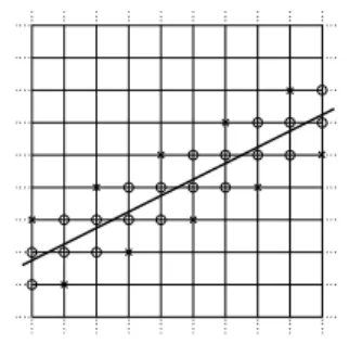
, where the four basic functions are (1±x)(1±y) in a local (x, y) frame. The displacement decomposition (4) is therefore particularized to account for the shape functions of a finite element discretization. For the enrichment, the choice proposed by Hansbo and Hansbo [6] is used (Figure 1). Each node of an element whose support is completely cut by the discontinuity holds an additional degree of freedom for each
component of the displacement associated with the function He
He(x) = H(x) − H(xe) (11)
where the vector xe gives the location of node e, and H is the Heaviside step function. Consequently,
the enrichment function He is equal to 0 over the area of the support of e (elements that have e within
their connectivity) on the same side of the crack as e. The main advantage of this function is that it avoids so-called blending elements (elements in which the enrichment is not supported by a partition of unity, i.e., elements that do not have all their nodes enriched). Furthermore, enriched terms of the matrix are only to be computed for the elements cut by the crack. Ill-conditioning may occur due to elements for which the enriched function is not vanishing over a small area. As a remedy, enriched degrees of freedom corresponding to nodes whose distance to the crack is about the element size are set to zero
and not considered as unknowns of the system. Those nodes are depicted using crosses on Figure 1. The numerical integration is performed pixel by pixel and any subdividing or special quadrature for the enriched elements are not needed. However, when a discontinuous kinematics is added to an element, the elementary matrix is to be computed over two different areas of the deformed image.
Figure 1. Discontinuous enrichment on a typical mesh. Circles denote nodes that hold discontinuous degrees of freedom, cross nodes that hold discontinuous degrees of freedom considered as fixed. Enrichissement discontinu sur un maillage. Les cercles correspondent `a des degr´es de libert´e avec discontinuit´es et les croix `a des degr´es de libert´e avec discontinuit´e gel´es.
2. Application to a bolted assembly
The X-Q4 algorithm is now applied to a practical configuration corresponding to a tensile test on a bolted assembly [7]. In the experiment, there are three aluminum plates assembled by a bolt. The previous algorithm is suited for the analysis of the displacement field on the edge of the sample. The region of interest is depicted in Figure 2-a. Upon loading, the central plate may slip with respect to the other ones, giving rise to two tangential discontinuities of the displacement along the interfaces. Only one (left side) of the two discontinuities is analyzed with the extended correlation algorithm. The other one is studied with a plain Q4 algorithm, where no enrichment is used. Thus we have a direct evaluation of the performance of the proposed enrichment. In the present case, the location of the discontinuity line is (easily) chosen by the user.
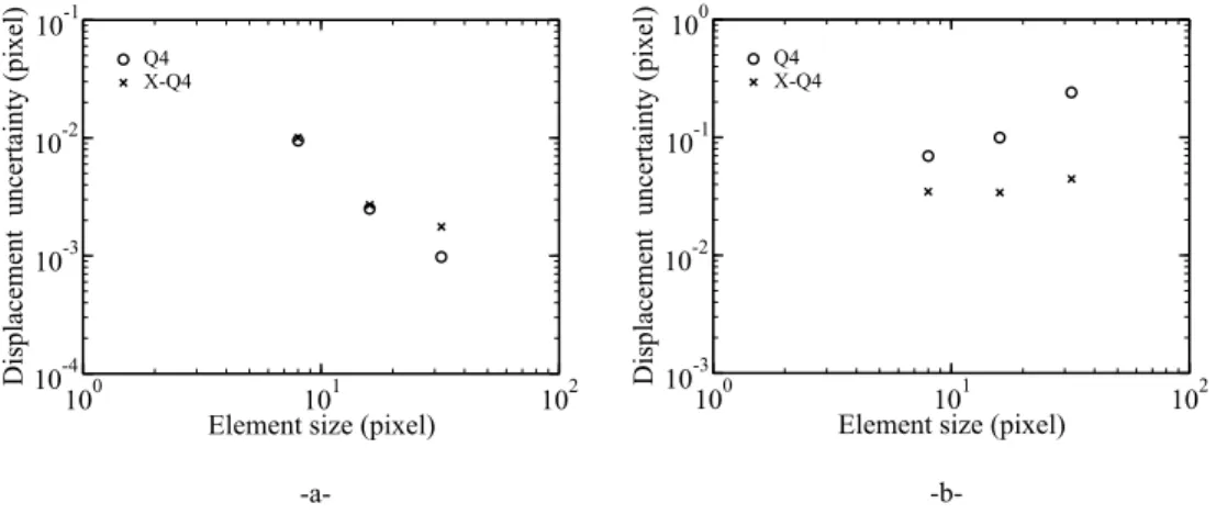
Before commenting the results, it is worth analyzing the performance of the correlation algorithm. A common baseline analysis consists in prescribing known displacements to the ROI and evaluate the displacement uncertainty [4]. Two cases are considered. First, a uniform displacement ranging from 0 to 1 pixel is prescribed. This allows one to estimate both the systematic and fluctuating parts of the error in the measured displacement. The fluctuation part is typically much larger, and thus only the latter is documented here, and quantified through the standard deviation of the displacement field. It is shown for both Q4 and X-Q4 algorithms in Figure 3-a. Even though the kinematic basis of the extended algorithm is richer than in the Q4 version, the overall performance is conserved. The only difference is that it levels
off earlier than the Q4 algorithm, yet at the very low value of 10−3 pixel. To capture without enrichment
a rapid variation of the displacement such as a discontinuity, a small element size would be needed, thus implying a rather large uncertainty. Conversely, with enrichment, the full benefit of the very small uncertainty attached to large element sizes is preserved without any prejudice to the description of the discontinuity.
The second configuration consists in applying a sub-pixel displacement discontinuity along a prescribed line. Figure 3-b shows that extended algorithm yields better results. The displacement uncertainty in-creases with the element size (when an element is cut by a discontinuity, the neighboring ones are also concerned because of the continuity of the shape functions). Conversely, the extended algorithm yields uncertainties that, in the present case, are roughly independent of the element size.
20 40 60 80 100 120 140 160 20 60 100 50 100 150 200 250 300 350 2.5 3 3.5 4 4.5 5 Ux (pixels) 20 60 100 50 100 150 200 250 300 350 0.2 0.3 0.4 0.5 0.6 0.7 Uy (pixel) 20 60 100 50 100 150 200 250 300 350 ROI x y Φ (gray levels) -a- -b- -c-
-d-Figure 2. -a-Analyzed bolted assembly and rectangular region of interest (ROI) delimited by a white dashed line. -b-Vertical displacement field in pixels. -c-Horizontal displacement field. -d-Gray level residual map. -a-Assemblage boulonn´e et r´egion d’´etude rectangulaire d´elimit´ee par un trait blanc discontinu. -b-Champ de d´eplacement vertical en pixels. -c-Champ de d´eplacement horizontal. -d-Carte de r´esidus en niveaux de gris.
100 101 102
Element size (pixel) -a-10-4 10-3 10-2 10-1 D ispla c ement u n c er taint y (pixel) Q4X-Q4 100 101 102
Element size (pixel) -b-10-3 10-2 10-1 100 D ispla c ement u n c er taint y (pixel) Q4X-Q4
Figure 3. Displacement uncertainties as a function of element size for a Q4 and an extended (X-Q4) algorithm when a uniform displacement is prescribed (a), and a discontinuous displacement (b). Incertitudes en d´eplacement en fonction de la taille des ´el´ements pour un algorithme Q4 et X-Q4 lorsqu’un champ constant (a) ou discontinu (b) est impos´e.
For the previous analysis, it is concluded that the displacement uncertainty is less than 0.05 pixel in the presence of a discontinuity. It is worth remembering that this result is related to the gray level distribution along the assumed discontinuity. In the present case, the latter is poor due to lighting conditions and the texture itself. When the element size is equal to 16 pixels, the displacement fields are shown in Figure 2-b,c. From the error map (Figure 2-d) it is concluded that the kinematics is well described by the extended algorithm (left discontinuity), whereas, as expected, the Q4 algorithm smears out the (right) discontinuity. The fact that the random texture is poor induces displacement fluctuations that are clearly visible on the horizontal displacement map.
The same type of analysis is performed by decreasing the element size (12 pixels and 8 pixels). The left discontinuity is still analyzed with an extended algorithm whereas the right one with a Q4 algorithm. As the element size decreases, the smeared out zone decreases (Figure 4). Conversely, the displacement field
0 20 40 60 80 100 120 140 20 60 100 140 50 100 150 200 250 300 350 2 2.5 3 3.5 4 4.5 20 60 100 140 50 100 150 200 250 300 350 2.5 3 3.5 4 4.5 20 60 100 140 50 100 150 200 250 300 350 0 20 40 60 80 100 120 140 160 20 60 100 140 50 100 150 200 250 300 350 Ux (pixels) Φ (gray levels)
-a- -b- -c-
-d-Φ (gray levels) Ux (pixels)
Figure 4. Vertical displacement field in pixels and corresponding error map in gray levels when the element size is equal to 8 pixels (a and b), 12 pixels (c and d). Champ de d´eplacement vertical en pixels et r´esidus correspondants lorsque la taille d’´el´ement est ´egale `a 8 (a et b) ou 12 pixels (c et d).
around the left discontinuity remains almost unaltered thanks to the extended algorithm. The fact that the displacement level along the discontinuity is significantly greater than the measurement uncertainty makes the results given by the extended algorithm less sensitive to the element size than those with a Q4 algorithm.
3. Summary and perspectives
An extended correlation algorithm was presented in this Note. It allows one to analyze situations in which discontinuities in the displacement field arise. It is the experimental counterpart to an enriched finite element kinematics. Sub-pixel and localized discontinuities are measurable. The algorithm was applied to study an experiment on a bolted assembly for which a much more accurate kinematic description is obtained as compared to a Q4 basis without enrichment.
The approach presented herein was particularized to describe a discontinuity that traverses the whole region of interest. It can be further generalized [as already exemplified by Eqn. (10)] to the analysis of cracked surfaces or even to the case of weak discontinuities. Furthermore, an automatic detection and optimization of the discontinuity geometry is desirable and will be presented in a forthcoming communi-cation.
Acknowledgements
This work is part of a project (PHOTOFIT) funded by the Agence Nationale de la Recherche. The authors wish to thank St´ephane Guinard, Nicolas Swiergiel and Julien Vignot of EADS for providing the pictures of the bolted assembly analyzed herein.
References
[1] P.K. Rastogi, ed., Photomechanics, Springer, Berlin (Germany), (2000).
[2] F. Hild, S. Roux, Measuring stress intensity factors with a camera: Integrated Digital Image Correlation (I-DIC), C.R. Mecanique 334 (2006) 8-12. See also, S. Roux, F. Hild, Stress intensity factor measurements from digital image correlation: post-processing and integrated approaches, Int. J. Fract. 140 (2006) 141-157.
[3] N. M¨oes, J. Dolbow, T. Belytschko, A finite element method for crack growth without remeshing, Int. J. Num. Meth. Eng. 46 (1999) 133-150.
[4] G. Besnard, F. Hild, S. Roux, “Finite-element” displacement fields analysis from digital images: Application to Portevin-Le Chˆatelier bands, Exp. Mech. 46 (2006) 789-803.
[5] I. Babuska, J.M. Melenk, The partition of unity method, Int. J. Num. Meth. Eng. 40 (1997) 727-758.
[6] A. Hansbo, P. Hansbo, A finite element method for the simulation of strong and weak discontinuities in solid mechanics, Comp. Meth. Appl. Mech. Eng. 193 (2004) 3523-3540.
[7] S. Guinard, N. Swiergiel, J. Vignot, Personal communication, 2006.