Computational insights into multivalently binding polymers

(1)

Computational Insights into Multivalently

Binding Polymers

by

Emiko Zumbro

S.B., Harvard University (2013)

Submitted to the Department of Materials Science and Engineering

in partial fulfillment of the requirements for the degree of

Doctor of Philosophy in Materials Science and Engineering

and the Program in Polymers and Soft Matter

at the

Massachusetts Institute of Technology

September 2020

© Massachusetts Institute of Technology 2020. All rights reserved.

Author . . . . Department of Materials Science and Engineering

August 7, 2020

Certified by. . . . Alfredo Alexander-Katz Associate Professor of Materials Science and Engineering Thesis Supervisor Accepted by . . . .

Frances M. Ross Chair, Departmental Committee on Graduate Studies

(2)

(3)

Computational Insights into Multivalently Binding Polymers

by Emiko Zumbro

Submitted to the Department of Materials Science and Engineering on August 7, 2020, in partial fulfillment of the requirements for the degree of

Doctor of Philosophy in Materials Science and Engineering and the Program in Polymers and Soft Matter

Abstract

Multivalent binding is commonly used throughout biology to create strong, conformal bonds using multiple weak binding interactions simultaneously. Bonds are considered multivalent when multiple ligands on one species simultaneously bind to multiple receptors on another species. Together, this bond can be much stronger than the sum of its parts. Throughout this thesis, we use theory and coarse-grain Brownian dynamics simulations with specific reactive-binding to explore general characteristics of multivalent polymer interactions. Our simulations bridge length and timescales and can sample large polymer systems that bind targets at the sub-nanometer lengthscale. While the simulation and theory presented is very general and can be applied to many diﬀerent systems of multivalent polymers, this thesis specifically explores consequences for two applications: multivalent polymers as decoys to inhibit infection and polymers as scaﬀolds for biocondensates.

Many pathogens use multivalent bonds to attach to our cell surfaces before entering and causing infection. Therefore, there is significant interest in preventing infection from viruses, bacteria, and toxic proteins by inhibiting this attachment step using multivalent decoys. There have been many experiments showing successful binding of long polymers or other large multivalent architectures to colloids or small proteins that pathogens use to bind to our cells. While these experiments have shown how promising multivalent inhibitors are for preventing infection, a theoretical understanding of why design parameters of multivalent polymers result in a particular binding aﬃnity is still missing. Simulations can easily isolate a single design parameter to provide direct links between structure and function, when experiments cannot always do so. This research is intended to provide a systematic study linking structure of multivalent polymers to their binding behavior.

In the first half of this thesis, we explore design properties of polymeric binders and how degree of polymerization, solvent quality, binding site affinity patterns, backbone stiffness, and target concentration change the multivalent binding affinity. We provide simple theory to show that multivalent polymers are limited by their ability and the energetic costs of forming polymer loops. We go on to show how these results and theory have implications on the binding affinity of polymers with heterogeneous binding sites and determines the effect of polymer backbone flexibility and solvent quality on binding affinity.

Multivalent polymers are also an essential component of biocondensates, liquid-like droplets comprised of proteins and nucleic acids are found throughout cells. Although the function of these biocondensates is still an active field of study, it is clear that multivalent polymers are essential to their formation through liquid-liquid phase separation (LLPS). There is lit-tle theoretical study of biocondensates that contain binding between species of asymmetric

(4)

size and valency and the eﬀects of multivalent polymers on the dynamics of these liquid droplets is not well understood. Studying how multivalent polymers modulate droplet dy-namics is important because droplet crystallization or solidification is often associated with neurodegenerative disorders such as dementia and amyotrophic lateral sclerosis (ALS).

Therefore, in the second half of this thesis, we present research on the role multivalent polymers play in LLPS droplets and their resulting dynamics. We consider how a host of design parameters can change the phase boundary of systems with multivalent polymers binding to smaller targets including solvent quality, valency, binding affinity, specific versus non-specific binding sites, and backbone stiffness. We found that consistent with previous work on other systems, asymmetric valency systems also showed increased phase separa-tion with increased binding affinities and valencies. We show that phase separasepara-tion due to non-specific bonds is highly sensitive to changes in attraction, but that phase separation through specific-bonds is much more robust. By combining specific and non-specific multi-valency, systems can precisely tune the phase separation boundary. Polymer stiffness can also modulate the phase boundary, where stiff, rod-like polymers were less able to cause phase separation than their flexible counterparts. We also elucidate how polymer-target binding affinities can be used to form micro-phase separated droplets. Lastly, we show that increasing attraction to polymers can slow target diffusion inside droplets while decreasing the density of droplets, with implications for droplet solidification.

We hope that this work will provide direction for the rational design of synthetic mul-tivalent polymer systems such as pathogen inhibitors as well as improve understanding of native biological systems like biocondensates.

Thesis Supervisor: Alfredo Alexander-Katz

(5)

Acknowledgments

This work could not have happened without the help of my many supporters.

First and foremost, I’d like to thank Alfredo for being the best advisor and friend a graduate student could ever ask for. Alfredo was first recommended to me as a great scientist and advisor before I became a graduate student when I was actually visiting another school, and he has definitely lived up to his reputation. I entered graduate school with no previous education on soft materials and no traditional laboratory experience, but Alfredo wasn’t deterred from welcoming me into his research group. Alfredo is a brilliant scientist, who has spent countless hours discussing research problems with me, practicing for qualifying exams, and teaching me polymer physics. No research problem is too small or too big for him to be fully dedicated to solving, and he always knew just what to say to encourage me when a project wasn’t going well or started to lose steam. Alfredo deeply cares about all of his students, as evidenced by him winning every award there is at MIT for his advising. He places equal emphasis on working hard and taking time for our families, our friends, and our wellbeing, all of which make up so much of the graduate student experience. His compassion and support have carried me through my graduate experience, and I could not be more grateful to him.

To the Alexander-Katz group: Shayna, Hejin, Karim, Mukarram, Shahrzad, Zhen, Josh, Yi, and Pierre, you are all amazing. I feel so lucky to have been a part of this group. When I joined the group, one of you told me that it was the best group because it is like a little family, and that couldn’t be more accurate. Even though all of our projects are separate, each of you would drop anything to help me on a research or homework problem I was stuck on, practice a conference talk, study for quals, or just take a snack break. Even after graduating and moving away, you’re still so generous with your time and energy. So much of my time here was shaped by having such wonderful people to share my oﬃce with, and I am very thankful to have gained such incredible lifelong friends throughout this experience.

Thank you to my thesis committee, Prof. Darrell Irvine, Prof. Katharina Ribbeck, and Prof. Jim Swan. You are all amazing scientists and have provided me with many insightful scientific suggestions over the past 5 years that have greatly improved the quality of my thesis research.

A huge part of the grad school is all of the wonderful people you meet outside of the lab, and I have met so many friends all over MIT. You have brought so much joy and fun to my graduate experience. A special thank you to Niels and the Holten-Andersen lab, the Ribbeck lab

(6)

who welcomed me with open arms and taught me everything they knew about mucus, the Polymer Graduate Student Association, TD’s cohort from Nuclear Science and Engineering, and all of the wonderful friends in my materials science cohort especially Hugo, PJ, and Irina.

To my friends from before grad school, thank you for constantly checking on me and making sure I sometimes left the MIT bubble. I feel your love and support always. You all inspire me every day with all the amazing things you’re accomplishing and I am excited to continuing watching you grow.

Thank you to my extended family, family friends, and in-laws. The MacDonald family treated me like one of their own since the first time I met them. They always make me smile when I need it, and I can’t imagine a family I could be happier to join. To my extended family and family friends, you have helped me every step of the way with your endless love and support. From Friday night dinners to helping with grade school science projects to putting together a last minute wedding, you have all contributed so much to getting me here. Thank you to Katy and Christina for making me an Aunt by giving us Tilly and Billie, and bringing so much happiness when our family needed it most.

Thank you to my siblings, Mari and Austin, who have been there since day 1, supporting me and challenging me to be the best person I can. Thank you for always stepping up when I need you, and for your endless love. Thank you to my mom and dad, for their unconditional love and support. Thank you for always pushing us to be the best we could be, for building the stable foundation and loving family that made this all possible, and thank you for for always being my biggest cheerleaders. With a dad as a math teacher and a mom as an elevator mechanic, one of your children had to turn out to be a scientist. I love you all so much and feel incredibly lucky to have you.

Last but not least, thank you to my husband TD for being there for every day of my PhD. The best part of this experience has been meeting you. You have been my rock and best friend throughout all of this, and I could not have done it without you. I love you very much.

(7)

List of Figures

1-1 Pathogenic proteins can bind to the complex sugars on the surface of our cells as one of the first steps of infection. Using multivalent polymers as decoys is a promising avenue for blocking the binding of pathogens and the resulting infection of healthy cells. In this work we are interested in how the properties of multivalent polymers change their binding to these toxic proteins. . . 40 1-2 Cells contain liquid-like droplets called biocondensates that contain multivalent

poly-mers and their cognate binding proteins. The multivalent polypoly-mers are depicted as RNA, but can also be linear multivalent proteins. We are interested in how properties of multivalent polymers can alter the phase separation that leads to these condensed droplets and the resulting dynamics of the droplet. . . 41 2-1 Polymers are represented by spherical beads (light blue) connected by gaussian springs.

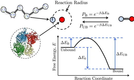
Each polymer bead has a single ligand. Targets can have multiple binding sites and are represented by a single spherical bead (red). Polymer ligands and target bind-ing sites interact when they are within a reaction radius that is dependent on the timestep. Within this reaction radius, they have a probability of binding PB that

depends on the depicted free energy landscape. Once bound, the target and poly-mer beads are connected by a gaussian spring, and with some probability PUB can

return to being unbound and interacting solely through a Lennard-Jones potential. Rendering from the Protein Data Bank [68,69]. . . 46 2-2 Simulated end-to-end distance of a polymer with degree of polymerization NP= 64

for various solvent qualities. The polymer has a size of 2apNP= 8, consistent with

(12)

2-3 A plot of the fraction of time bound for diﬀerent monomeric polymer bead concen-trations interacting with a monovalent target. By fitting to the Langmuir adsorption curve [P ]/([P ] + KD) (dashed lines), we can find the KD of monovalent binding

cor-responding to the values of E0 noted in the plot legend. Simulation results (circles)

and Langmuir adsorption equation fits (dashed lines) are shown for E0= 2, 3,

4, 5, and 6kBT. When results are rescaled to Molar using an estimated target

diameter of 5 nm, the KD for these binding energies is in the mM to µM range typical

of monovalent glycan – lectin and some protein - nucleic acid binding interactions [81–85]. Fit values of KD are shown above their corresponding lines. . . 50

3-1 Schematic of the scenarios tested when comparing binding avidity’s dependence on degree of polymerization. The volume and number of inhibitor ligands are held constant to maintain a constant concentration of ligands at 64 ligands per box. The connectivity of the inhibitor ligands was varied from monomers to 64mers in multiples of two so that degrees of polymerization, 1, 2, 4, 8, 16, 32, and 64 were all investigated. This ensured that all polymers in each simulation were monodisperse. . . 55

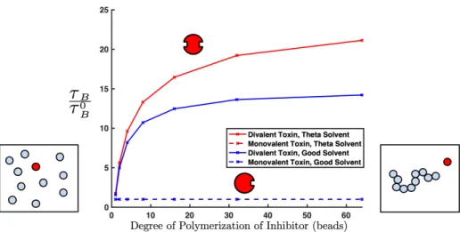
3-2 Average time interval a monovalent or divalent target are bound to polymeric in-hibitors of various lengths, normalized by the average time bound for a monovalent target, ⌧0

B. The time interval bound for a monovalent toxin does not depend on the

in-hibitor length (dashed blue line and dashed red line overlap). For the divalent target (solid), oligomeric inhibitors spend significantly more time bound than monomeric inhibitors, exhibiting the enhancement of multivalent binding avidities over mono-valent binding. At high degrees of polymerization of the inhibiting polymer, as the length of the inhibitors is increased further, there is only a small gain in the average time interval the target is bound. The time spent bound approaches some maximum value with increasing inhibitor length. Inhibitors in theta solvent (red, Case 1 in Table 3.1) spend more time bound than good solvent (blue, Case 2 in Table 3.1). Error bars are smaller than symbol size. . . 56

(13)

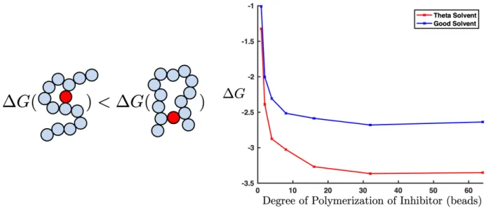
3-3 A plot of the free energy of binding for the degree of polymerization of the inhibitor. The free energy of binding is calculated using the average time interval the target spends bound to the polymer ⌧B(meaning one or more binding sites is bound) divided

by the average time interval the target spends completely unbound ⌧UB. Longer loops

are entropically unfavorable, so while they are possible in longer polymers, they are unlikely to form. We can see that this leads to a limiting minimum binding energy as degree of polymerization of our inhibitor increases. This is true in both good (blue) and theta (red) solvents. . . 57

3-4 Log-log plot of the percent of time a divalent target forms various loop sizes for diﬀerent length polymers. For reference, 1% frequency is shown with dashed black line. In theta solvent (A) and good solvent (B), loops larger than 13 and 9 beads, respectively, are formed less than 1% of the time. mref = 3⌫ is a reference slope

where ⌫ is the Flory exponent. . . 58

3-5 Schematic of the scenarios tested when comparing binding avidity’s dependence on degree of polymerization with multiple targets present. The volume and number of inhibitor ligands are held constant to maintain a constant concentration of ligands at 64 ligands per box. The connectivity of the inhibitor ligands was varied from monomers to 64mers in multiples of two so that degrees of polymerization, 1, 2, 4, 8, 16, 32, and 64 were all investigated. This ensured that all polymers in each simulation were monodisperse. The concentration of targets was held constant in all simulations. 60

3-6 Plot of average time bound (⌧B) for targets when multiple targets are present.

Y-axis is normalized by the average time bound for monomeric inhibitors, ⌧0

B. Data

presented is for polymer-target binding energy of E0 = 4 kBT in theta solvent.

Similar to with a single target, ⌧Bhas a limited increase with degree of polymerization

of the inhibiting polymer. More attractive inter-target potentials (orange, ✏TT = 18₁₂)

(14)

3-7 Distribution of times spent bound for single target scenarios (yellow) and scenarios with multiple targets (orange and blue). The rate of unbinding corresponds to the slope of the line in these two regions, shown in black. There is a fast and a slow timescale on which targets unbind. The former corresponds to singly bound targets unbinding and does not change with inter-target potentials. The second, longer timescale corresponds to doubly bound targets that unbind. When there are favorable target-target interactions (orange), the decay in doubly bound times is faster than if there is not an attraction between targets (blue), or if there is no competition from other targets (yellow). . . 62 3-8 There are two types of competition bound targets experience that lead to shorter

times bound for divalently bound targets. (A) shows competition from neighboring bound targets and (B) shows competition from nearby unbound targets which is increased for more favorable inter-target potentials. . . 63 3-9 Percent of inhibitor beads bound in theta solvent when the target-polymer binding

aﬃnity is E0 = 4kBT (A) and 2kBT (B). (A) As inhibitor length increases, a

transition occurs that allows the polymer to bind a significantly higher percentage of targets when there is some inter-target attraction. This transition happens at approximately degree of polymerization of 10 for monovalent targets and degree of polymerization of around 3 for divalent targets. (B) At very low polymer-target binding aﬃnities, such as 2kBT, a critical percentage of targets never bind to the

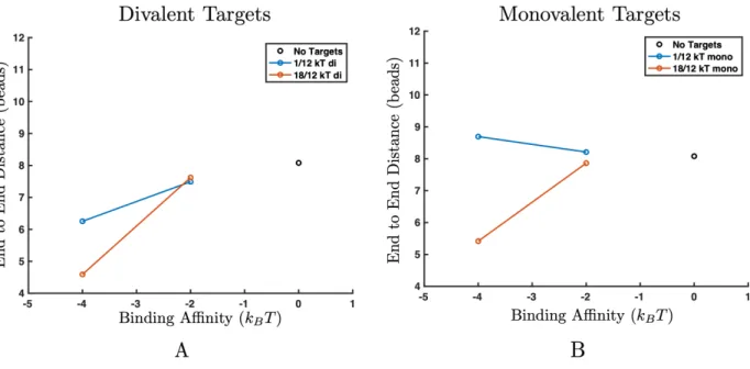
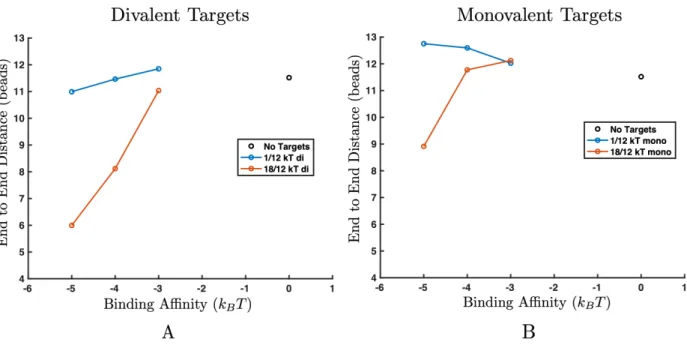
inhibiting polymer, so even at high degrees of polymerization, a transition in binding does not occur. Error bars are smaller than symbol size. . . 64 3-10 End to end distance for 64-mer polymers in theta solvent in the presence of

diva-lent targets (A) and monovadiva-lent targets (B). (A) Increasing binding aﬃnity between the targets and polymers induces a transition where the polymer collapses in size for both inter-target attractions. (B) Only high inter-target attraction leads to a collapse transition (orange). Low inter-target attraction (blue) does not provide enough en-thalpic gain to overcome the entropic loss of phase separation. Error bars are smaller than symbol size. . . 65

(15)

3-11 The amount of time each inhibitor bead spends bound when interacting with monova-lent, 4 kBT binding targets. Plots compare binding times for monomeric inhibitor

beads (red) and beads that are part of a 64-mer polymer (blue). (A) Time bound when interacting with targets that have low (✏ = 1/12 kBT) target-target attraction.

Monomers are each bound for a uniform amount of time, but the polymer ends are bound much more frequently than the polymer beads in the center of the chain. (B) When interacting with targets that have higher target-target attraction (✏ = 18/12 kBT), the polymer collapses, making the center beads bound more frequently than

the chain ends. Monomeric inhibitor beads continue to experience uniform binding preference. . . 66

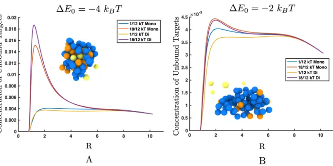
3-12 Plot of the minimum distance away from the polymer that unbound targets are found, normalized by the volume of a sphere with radius R, where R is the distance the center of the target is from the center of the nearest polymer bead. Data is shown for 64mer polymers in theta solvent with polymer-target binding aﬃnities of (A) 4kBT and

(B) 2kBT. (A) The concentration of unbound targets is approximately the same as

the bulk when there is low inter-target attraction, but the concentration of unbound target near the polymer is higher than the bulk concentration when the inter-target potential is increased. The rendering in the inset shows unbound targets (yellow) clustered inside the polymer (blue) by the bound targets (orange). (B) Fewer targets have bound to the polymer, so the polymer has not collapsed. This makes the local concentration of unbound targets near the polymer approximately the same as the bulk concentration for both high and low inter-target attractions. . . 67

3-13 Percent of inhibitor beads bound in good solvent when the target-polymer binding aﬃnity is 4 kBT. As inhibitor length increases, fewer monovalent targets (blue) are

bound for both inter-target attractions because the enthalpic gain of targets binding does not overcome the loss of entropy. For divalent targets (red), longer polymers lead to an increase in binding avidity with higher inter-target attraction. . . 68

(16)

3-14 End to end distance for 64-mer polymers in good solvent in the presence of divalent targets (A) and monovalent targets (B). (A) Increasing binding aﬃnity between the targets and polymers induces a collapse transition where the polymer distinctly col-lapses in size for higher inter-target attractions. This collapse in good solvent occurs at a stronger target-polymer binding aﬃnity than in theta solvent. (B) Only high target attraction leads to a transition where the polymer collapses. Low inter-target attraction does not provide enough enthalpic gain to overcome the entropic loss of phase separation. . . 69 3-15 Plot of the minimum distance away from the polymer that unbound targets are

found, normalized by the volume of a sphere with radius R, where R is the distance the center of the target is from the center of the nearest polymer bead. Data is shown for polymer-target binding aﬃnity of 4 kBT in good solvent. The concentration of

unbound targets is approximately the same as the bulk when there is low inter-target attraction, but the concentration of unbound target near the polymer is higher than the bulk concentration when the inter-target potential is increased. This clustering of unbound targets is slight for monovalent targets because the polymer has not gone through a collapse transition, but unbound target clustering is significant for divalent targets because the polymer end to end distance has been greatly reduced. . . 70 4-1 Multivalent polymers have shown promise as inhibitors for toxic lectins by preventing

their attachment and subsequent infection to cells, as shown in the right panel. . . . 73 4-2 Schematic of simulation. The globular protein target is approximated as a sphere with

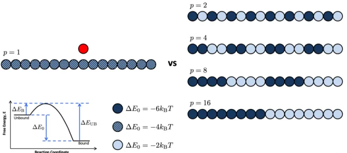
one or more binding sites. The polymeric inhibitor is represented by a bead spring model where each bead has a single binding site and is connected to its neighbors through harmonic springs. Rendering from the Protein Data Bank [68,69]. This figure is reprinted from Zumbro et al. with permission from Elsevier [86]. . . 75 4-3 Schematic of the polymer patterns tested when exploring binding of a target (red)

to homopolymers and copolymers (blues). The periodicity, p is labeled above each polymer pattern. Here, dark circles indicate high aﬃnity binding sites with E0 =

6kBT, light circles represent low aﬃnity binding sites with E0 = 2kBT, and

striped circles represent a medium binding aﬃnity used only for the homopolymer comparison with E0= 4kBT. . . 77

(17)

4-4 Plot of the average time bound ⌧B vs the periodicity of the polymer p. The binding

dependence on polymer pattern is diﬀerent for divalent targets (blue) and monova-lent targets (orange). Periodically patterned polymers are represented by connected circles (-o), homopolymers are represented as x’s (x), and random copolymers are represented by squares (⇤). Because the binding of 100 co-polymer patterns were averaged, the standard deviation of the ⌧B across random polymer patterns is

de-picted as error bars. The eﬀect of pattern is also dependent on the concentration of targets. (A) At dilute target concentrations, target binding increases with copolymer periodicity but (B) at higher target concentrations low periodicity copolymers have higher ⌧B. The sampling error for all data points is smaller than the symbol size. . . 78

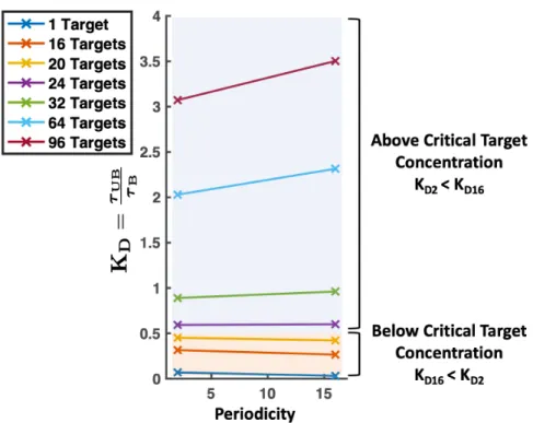
4-5 Frequency that a polymer bead is bound throughout the simulation when (A) a single divalent target and (B) 64 divalent targets are present for homopolymers (blue), alternating copolymers (red), and blocky copolymers (green). (A) For the patterned copolymers, low affinity binding sites are bound with almost the same frequency. However, the high affinity binding sites on the blocky polymer are bound much more frequently than the low affinity binding sites on the alternating polymer. (B) For the patterned copolymers, attractive binding sites are bound with almost the same frequency. However, the low affinity binding sites on the blocky polymer are bound much less frequently than the low affinity binding sites on the alternating polymer. Error bars are smaller than the symbol size. . . 80 4-6 Dissociation constant KD versus periodicity of polymer pattern for target

concen-trations from 1 to 96. We have marked the concenconcen-trations below the critical target concentration where the blocky polymer (p = 16) has a KD less than that of an

al-ternating polymer (p = 2) with an orange background. The values above the critical target concentration where the alternating polymer has a lower KD than the blocky

polymer has been labeled with a blue background. . . 83 4-7 Frequency monovalent targets are bound to binding sites on homopolymers and

copolymers with alternating and blocky patterns. Results are shown for (A) when a single target is placed with 4 16mer inhibiting polymers and (B) when 64 targets are placed with 4 16mer inhibiting polymers. Frequency of time bound depends on the aﬃnity of that polymer binding site and not on polymer binding site pattern. . . 86

(18)

4-8 Dissociation constant for alternating (p = 2) and blocky (p = 16) polymers with E0 pairs (0, 6kbT), ( 2, 6kbT), and ( 3, 5kbT). All data shown is for high

competition simulations with 64 targets. . . 87

4-9 Fraction of all time spent bound that a target is bound divalently for a single target interacting with four polymers in orange (-⇤) and for 64 targets interacting with polymers in blue (-⇤). Fraction of time bound is also plotted for all three divalent bond types: two high affinity bonds (–x), two low affinity bonds (–⇤), and bonds with one low and one high affinity bonds, labeled as “Both" in the legend (–o). Values are shown for two polymer periodicities where (p = 2) is an alternating polymer and (p = 16) is a block copolymer. . . 89

5-1 Depiction of simulation scheme. Polymers are represented by spherical beads (light blue) connected by harmonic springs. To introduce stiﬀness, we employ a simple scheme used also by some commonly utilized force fields (e.g. MARTINI [119]), where an additional spring is placed between every next nearest neighbor along the chain. Each polymer bead has a single ligand, meaning it can only bind monovalently, but making the polymer as a whole multivalent. Targets, on the other hand, can have multiple binding sites and are represented by a single spherical bead (red) with one or two binding sites as shown. Polymer ligands and target binding sites interact when they are within a reaction radius. Within this reaction radius, they have a probability of binding PB that depends on the free-energy landscape, as depicted. Once bound,

the target and polymer bead are connected by a harmonic spring, and they can unbind with probability, PUB. Apart from the reactive kinetics that we include here to model

the specific binding mechanisms, we use a Lennard-Jones potential to maintain the chain conformation and prevent target-target and target-polymer overlap. This figure is adapted from Zumbro et al. with permission from Elsevier [86]. . . 95

(19)

5-2 Simulated average end-to-end distance R of 16mer polymer chain normalized by the contour length L0 plotted versus chain stiﬀness spring coeﬃcient is shown as blue

X’s. Values of R and at which simulations were run are highlighted with dashed lines. These values of were chosen to explore a wide range of polymer flexibilities and represent the point where R ⇡ 4 for a perfectly flexible polymer, and 25%, 50%, and 75% of the distance between the most flexible chain R ⇡ 4 and a perfectly rigid rod where R = L0 = 15. End-to-end distances were converted to C1 on the right

axis and persistence length, p on the top axis using the empirical wormlike chain fit relating R/L0 to p/L0 (black solid line) [121,55]. . . 96

5-3 (A) Schematic of the single target simulation set up with a single mono- or divalent target shown in red and four polymers with a length of 16 beads. (B) The average time interval bound ⌧B of a single divalent target (blue) and a monovalent target

(orange) versus the polymer stiffness controlled by the angle-bending spring coefficient . Higher corresponds to stiffer springs and more rigid polymers. The monovalent target ⌧B seems unaffected by the polymer chain stiffness while the divalent targets

show a decrease in ⌧B with . Error bars are smaller than symbol size. . . 98

5-4 Percent of time that a polymer bound twice to a target is in a certain loop length plotted in (A) log-log scale and (B) log-linear scale. Each color represents a different polymer stiffness, the dashed black line represents 1%, and the solid black line is an example of y = x 1.8_{. The frequency of long loops decreases as polymer stiffness}

increases. (A) More flexible chains ( = 0, 1) have a power law decay in loop size due to the entropic cost of forming loops[86]. This manifests as a straight line in the log-log scale. (B) Stiﬀer chains ( = 4.3, 7.65) have an exponential decay in loop lengths for short loops due to the energetic cost of bending. We can see this manifest in the log-linear plot as a straight line for short loop lengths (lloop = 1, 2, 3). Lines

are for aiding the eye and are not a theoretical fit. . . 100 5-5 Frequency of loop sizes in Log-Linear scaling. ‘x’s denote simulation data and dashed

( ) lines represent the best linear fit following equation 5.3 with values of C1 and

C2listed in Table 5.2 and 5.3. (A) Loop data and linear fits for matched size polymer

and target beads (aP= 0.5, aT = 0.5). (B) Loop data and linear fits for mismatched

bead sizes with smaller polymer beads and larger target bead (aP= 0.25, aT = 1.0)

(20)

5-6 (A) The average time interval unbound ⌧UB for a single mono- (orange) or divalent

(blue) target binding to a polymer. The ⌧UBdecreases similarly for both target

valen-cies because it is dependent on the distribution of polymer binding sites throughout the simulation volume. Standard error is denoted by error bars. (B) Dissociation constant KD for a divalent target versus polymer stiﬀness. The longer ⌧UB is not

enough to overcome the longer ⌧B for flexible polymers and flexible polymers show a

lower KD(higher aﬃnity) than rigid ones. A plot of the KDfor a monovalent target

is dominated by ⌧UB and is shown in Figure 5-16. . . 104

5-7 Schematic of simulations with multiple targets. In this case, 32, 64, 96, or 128 targets are placed in a box with four 16mer polymers to examine how target-target interactions and competition between targets for binding sites on the polymer can change the phase behavior of the system. . . 105

5-8 Phase diagrams of (A) targets only with increasing concentration of targets on one axis and increasing target-target Lennard-Jones attraction on the other and (B) sim-ulations of 96 targets mixed with four 16mer polymer. To highlight the change in phase separation with stiﬀness, the polymer stiﬀness on one axis and target-target Lennard-Jones attraction on the other. Results are shown for both mono and divalent targets. Not phase separated or “mixed" systems are denoted by a red letter “N" for “no", a phase separated system where the polymer and targets are both components of the condensed phase is denoted by a green “Y" for “yes", and a purple “Y" denotes a system where the targets phase separated by themselves, in this case because no polymer was added. Regions where targets can phase separate by themselves, with-out the help of the polymer are shaded with a purple background. Systems where phase separation only occurs through interaction between polymers and targets we call "co-phase separation" and is shaded with a blue background. . . 107

(21)

5-9 Phase diagrams of divalent targets mixed with four 16mer polymers with increasing concentration of targets on one axis and increasing target-target Lennard-Jones at-traction on the other. Phase diagrams are shown for five polymer flexibilities. Phase separation occurs at lower energies and target concentrations for flexible polymers than stiﬀ polymers. Not phase separated or “mixed" systems are denoted by a red letter “N" for “no", a phase separated system where the polymer and targets are both components of the condensed phase is denoted by a green “Y" for “yes", and a pur-ple “Y" denotes a system where the targets phase separated by themselves, without polymers. Regions where targets can phase separate by themselves, without the help of the polymer are shaded with a purple background. Systems where phase separa-tion only occurs through interacsepara-tion between polymers and targets we call “co-phase separation" and is shaded with a blue background. . . 108

5-10 (A) KD for 96 divalent targets binding to four 16mer polymers. As target-target

attraction ✏TT increases, KD decreases. For ✏TT= 1.0, binding aﬃnity is dominated

by the increased ⌧UBand flexible polymers are slightly lower aﬃnity than stiﬀ ones.

At ✏TT 1.5, ⌧B dominates and flexible polymers have higher aﬃnity than stiﬀ

polymers. We can see a sharp increase in KD for ✏TT = 1.7 as increases from 4.3

to 7.65 signaling the phase boundary where flexible polymers are able to nucleate a condensed target phase but stiff polymers are not. (B) Binding efficiency of polymers calculated as the average fraction of sites on the polymer bound versus . This plot closely mimics the one for KD, with a sharp decrease in binding efficiency for divalent

targets at ✏TT = 1.7 denoting the phase transition between = 4.3 and 7.65. For

phase separated systems at ✏TT = 2.0, there is an approximately 10% decrease in

sites bound on the polymer between the = 2.25 and = 7.65 for both target valencies. This is due to rigid polymer resistance to bending and their tails sticking out away from the condensed phase as shown in Figure 5-8B. Error bars are smaller than symbol size. . . 111

(22)

5-11 Radial distribution function (RDF) for concentration of unbound targets found near the polymer chain where the x-axis R is the distance from a target center of the closest polymer bead. Data is for 96 divalent target simulations. In all plots, the dashed line represents low target-target interaction ✏TT = 1.0. (A) The solid lines represent the

RDF of targets for ✏TT = 1.5. Only small changes in the RDF occur with stiﬀness.

(B) The solid lines represent the RDF of targets for ✏TT = 1.7. Note that the solid

blue, red, and yellow ( = 0, 1, 2.25) lines overlap. Here, flexible polymers show a much higher concentration of unbound targets near the chain because they are able to induce phase separation at this target-target potential. (C) The solid lines represent the RDF of targets for ✏TT = 2.0. Note that the blue, red, yellow, and purple lines

overlap ( = 0, 1, 2.25, 4.3). All polymers cause phase separation at this ✏TT, so all

flexibilities show increased concentration of unbound targets near the polymer. . . . 113

5-12 Phase diagrams of monovalent and trivalent targets mixed with four 16mer poly-mers with increasing concentration of targets on one axis and increasing target-target Lennard-Jones attraction on the other. Phase diagrams are shown for five polymer flexibilities. Phase separation occurs at lower energies and target concentrations for flexible polymers than stiﬀ polymers. Not phase separated or “mixed" systems are denoted by a red letter “N" for “no", a phase separated system where the polymer and targets are both components of the condensed phase is denoted by a green “Y" for “yes", and a purple “Y" denotes a system where the targets phase separated by them-selves, without polymers. Regions where targets can phase separate by themthem-selves, without the help of the polymer are shaded with a purple background. Systems where phase separation only occurs through interaction between polymers and targets we call “co-phase separation" and is shaded with a blue background. . . 115

5-13 Example of a typical system energy profile over time. The total energy is shown for a system with four 16mer polymers and 96 divalent targets with a target-target attraction ✏TT = 1.7kBT. Simulation energy is shown every 10000 timesteps. There

is an initial large drop in energy while the system equilibrates. Production research data is taken from the second half of the simulation, past this equilibration time period.117

(23)

5-14 Flux of an unbound target toward a cylinder (orange) and sphere (blue) vs the system volume. The cylinder and sphere represent a rigid and flexible polymer respectively. At the simulation volume per polymer ( black line), the diﬀusive flux toward the cylinder (rigid polymer) is greater than the diﬀusive flux toward the sphere (flexible polymer). . . 119

5-15 (A) Average time interval bound ⌧B and (B) unbound ⌧B for 96 targets. Monovalent

targets are shown in orange and divalent targets are shown in blue, with diﬀerent values of ✏TT denoted by diﬀerent line styles and points. (A) Divalent targets see a

decrease in ⌧B with increasing ✏TT due to additional competition for sites between

targets. Nucleation of a condensed polymer/target phase also results in increased competition, lowering the ⌧B more than in the mixed/not phase separated state.

Monovalent target ⌧B is unaﬀected by stiﬀness or phase separation and lines for

all ✏TT overlap. (B) For mixed systems, where no condensed phase is nucleated,

⌧UB is dominated by diﬀusion and flexible polymers with spherical morphology

ex-perience longer ⌧UB than rigid polymers for both divalent and monovalent targets.

When systems are phase separated, flexible polymers have slightly shorter ⌧UB than

stiﬀ polymers, likely due to a higher concentration of polymer binding sites in the condensed phase. Stiﬀ polymers lower their concentration of binding sites in the condensed phase by extending their tails away from the targets as shown in Figure 5-8B and 5-9. Error bars are smaller than symbol size. . . 119

(24)

5-16 Dissociation constant KDof monovalent targets for the single target case (A) and the

96 target case (B). (A) For one monovalent target, KD is dominated by the time it

takes the target to diﬀuse to a polymer. Because it takes longer for a target to diﬀuse to a sphere than to a rod, ⌧UB is longer for flexible polymers than rigid polymers, so

flexible polymers are lower aﬃnity (higher KD) for dilute monovalent targets. (B)

For 96 monovalent targets, systems that don’t phase separate behave similarly to the single target case; flexible polymers have lower aﬃnity (higher KD) than stiﬀ

polymers. When the system phase separates at ✏TT = 2.0kBT, flexible polymers

become higher affinity (lower KD) than stiff polymers because stiff polymers extend

away from the condensed target and are therefore bound less eﬃciently with a lower concentration of polymer binding sites in the condensed droplet. At ✏TT = 1.7kBT,

flexible polymers are significantly higher affinity than stiff polymers because they can induce phase separation at  4.3 while stiff polymers ( = 7.65) cannot. Error bars are smaller than symbol size. . . 120

5-17 Percent of time the divalent target spends bound in loops between two polymers (inter-polymer) out of all loops formed. (A) Results for the single target case. Stiﬀer polymers have a higher percentage of inter-loops than flexible polymers, likely due to the energetic cost of bending for stiﬀ polymers to form intra-polymer loops. (B) Results for 96 targets. For low inter-target attraction (blue, ✏TT = 1.0) and systems

where all polymer stiﬀnesses are phase separated (purple, ✏TT = 7.65), behavior is

similar to single target case where stiﬀness increases inter-polymer crosslinks. For ✏TT = 1.7 (yellow), flexible polymers have more crosslinks than stiﬀ ones. In this

case, more flexible polymers lead to droplets at ✏TT = 1.7 which brings polymer

chains close together in a condensed phase and reduces the penalty for bonds across two polymers. At ✏TT = 1.5, flexible polymers are likely on the verge of phase

separation and there are some transient small polymer-target droplets even though they don’t nucleate a stable condensed phase. We suspect that crosslinks might occur less in phase separated systems with ✏TT = 2.0than in ✏TT = 1.7because the targets

can phase separate by themselves and exclude the polymer from the droplet center through microphase separation. The eﬀects of microphase separation will be explored in future work. . . 122

(25)

5-18 Percent of time a bound target has both binding sites bound simultaneously versus polymer stiﬀness. A target is considered bound if one or more of its binding sites is occupied. Data is shown for 96 divalent targets binding to four 16mer polymers. Lines represent constant target-target attraction. Error bars are smaller than symbol size. . . 123 5-19 Simulation results for divalent targets with = 0. Data is shown for 32, 64, 96,

and 128 divalent targets interacting with four 16mer polymers with target-target attractions ranging from ✏TT = 1.0 to 2.0. Lines connect points of constant target

concentration. (A) Average energy of the system. (B) Binder cumulant. (C) Average Rg of all polymer beads relative to the collective system center of mass. (D) Average

Rg of each individual polymer relative to its own center of mass. . . 124

5-20 Simulation results for divalent targets with = 1.0. Data is shown for 32, 64, 96, and 128 divalent targets interacting with four 16mer polymers with target-target attractions ranging from ✏TT = 1.0 to 2.0. Lines connect points of constant target

(26)

5-24 Simulation results for monovalent targets with = 0. Data is shown for 32, 64, 96, and 128 monovalent targets interacting with four 16mer polymers with target-target attractions ranging from ✏TT = 1.0 to 2.0. Lines connect points of constant target

5-25 Simulation results for monovalent targets with = 7.65. Data is shown for 32, 64, 96, and 128 monovalent targets interacting with four 16mer polymers with target-target attractions ranging from ✏TT = 1.0 to 2.0. Lines connect points of constant target

5-26 Simulation results for trivalent targets with = 0. Data is shown for 32, 64, 96, and 128 trivalent targets interacting with four 16mer polymers with target-target attractions ranging from ✏TT = 1.0 to 2.0. Lines connect points of constant target

5-27 Simulation results for trivalent targets with = 7.65. Data is shown for 32, 64, 96, and 128 trivalent targets interacting with four 16mer polymers with target-target attractions ranging from ✏TT = 1.0 to 2.0. Lines connect points of constant target

(27)

6-1 Depiction of simulation scheme. Polymers are represented by spherical beads (light blue) connected by harmonic springs. These polymers could represent either nucleic acids or long modular binding proteins found in biocondensates. Each polymer bead has a single binding ligand. Target binding proteins are represented as spherical beads (red) and can have multiple binding sites (BS) depicted as green blocks. These protein beads also encompass a intrinsically disordered region (IDR) that modulates their non-specific attraction to the polymer and between the proteins themselves. When the polymers and binding proteins are mixed together, they can undergo a phase transition into a condensed droplet. . . 136

6-2 Two types types of protein-polymer interactions are explored in this work. (A) Non-specific excluded volume interactions controlled by a Lennard-Jones potential. These potentials are not valence limited and are felt by any target or polymer bead in accordance with their distance apart r. (B) Specific, valence-limited, lock-and-key type binding. Polymer ligands and target protein binding sites interact when they are within a reaction radius that is dependent on the timestep. Within this reaction radius, they have a probability of binding PBthat depends on the depicted free-energy

landscape. Once bound, the target and polymer bead are connected by a harmonic spring, and with some probability, PUB, can return to being unbound and interacting

solely through a Lennard-Jones potential. This figure is adapted from Zumbro et al. with permission from Elsevier [86]. . . 137

(28)

6-3 Properties of a single species alone, before mixing them together. (A) Average end-to-end distance of a 64mer polymer under various Lennard-Jones attractions ✏PP.

The polymer behaves as it would in ✓ conditions, as a perfect random walk, when ✏PP = ₁₂5. ✏PP = 8.5₁₂ is highlighted with an arrow to denote the attraction at which

four 16mer polymers aggregate into a single condensate. From this, we can see there is a region of poor solvent where polymers are collapsed but still soluble. (B) Phase diagram showing solubilities of binding proteins alone. When targets form a condensed phase without polymer, it is denoted with a purple "Y", and when they do not form a condensed phase, it is denoted with a red "N". From this chart, we see that all target concentrations tested are phase separated when ✏TT = 3.0, no

target concentrations nucleate a condensed phase at ✏TT = 1.7, and only high target

concentrations 96 and 128 targets phase separate at ✏TT = 2.0. This phase diagram

will serve as a control for the eﬀects of mixing polymers and target proteins. . . 138

6-4 Phase diagram resulting from specific lock-and-key binding to four 16mer polymers. Results are shown for mono, di, and trivalent binding proteins with E0= 2, 4, and

6kBT. Letters and letter coloring were determined by visual inspection, with example

renderings shown on the left of “Mixed" states labeled as a red “N" for no phase separation, fully phase separated systems with both polymers and proteins found in the condensed phase labeled with a green “Y" for yes phase separated, and purple ‘Y"s denoting systems in which a single species phase separated without the other such as the proteins condensing on their own. Yellow “Y"s denote systems in a the crossover region between phase separated and mixed where 60% of simulations showed a stable condensed droplet. Purple background shading denotes regions where pure protein simulations phase separated on their own without the help of the polymer. Blue background shading denotes the regions where phase separation was also indicated by Binder cumulant of the system energy. Yellow background shading denotes that aggregation of polymers into a droplet was indicated by a significant drop in the total Rg of the polymer system accompanied by a reduction in the Rg of individual

polymers. Phase separation occurs at lower protein target concentrations and lower ✏T T as valency and binding aﬃnity are increased. . . 140

(29)

6-5 Examples of simulation properties for divalent protein targets with four 16mer poly-mers in theta solvent and E0 = 6kBT, shown with lines of protein concentration.

(A) Total average energy of simulation (B) Binder cummulant comparing average energy fluctuations to average system energy. A maximum in the Binder cumulant corresponds to a phase boundary. (C) Rg of all polymers in the system. A large

reduction in system Rg signifies that all four polymers aggregated into a single body.

(D) Average Rg of individual polymers across the simulation time. A reduction in

Rg signifies a change in eﬀective solvent conditions for the polymer as a result of

complexation with binding proteins. After a critical concentration of protein binding is achieved, the polymers swell if the simulation isn’t protein concentration-limited. (E) Number of polymer sites bound with a maximum of 64. A plateau in sites bound occurs when a protein-polymer droplet is formed because the local concentration of protein targets reaches a maximum. (F) Variance in polymer binding sites occupied normalized by the average number of sites bound. The variance also plateaus when a condensed droplet is formed due to the smaller fluctuations in local concentration of proteins near the polymer in a liquid droplet. . . 141

6-6 Phase diagrams for polymers of diﬀerent of degrees of polymerization Np = 4 (Top

Row), 16 (Middle Row), and 64 (Bottom Row) with reactive, specific binding aﬃnities E0 = 4 and 6kBT. All simulations are for divalent proteins targets and theta

solvent for the polymer. Letter color coding and area shading have the same meanings as described in Figure 6-4. . . 144

6-7 Phase diagram of simulations comparing the behavior of four 16mer polymers with lock and key binding to divalent protein targets in theta solvent (✏PP= 5/12) to two

types of poor solvent (✏PP = 6/12 and 7/12). Polymers do not phase separate on

their own at any values of ✏PP tested. Lettering color codes and shading follow the

same key as Figure 6-4, with “Y"s indicating “yes" phase separation occurred and “N"s representing “no" phase separation occurred. In poor solvent, phase separation occurs when polymers are mixed with binding targets at lower ✏TTs and protein

(30)

6-8 Phase diagram for proteins binding to polymers through a non-specific Lennard-Jones potential. Diagrams use the same key described in detail in Figure 6-4 where phase separated systems are marked with a “Y" for “yes" and not phase separated systems are marked with an “N" for “no". Results are shown for simulations with increasing polymer binding attractions ✏TP from left to right (columns) with four

16mer polymers (Top) and one 64mer polymer (Bottom). . . 147

6-9 Phase diagram of targets and polymer with both nonspecific binding aﬃnity ✏TP =

5/12and specific lock and key binding (Bottom Row) compared with polymers that have lock and key binding but almost no non-specific attraction to the targets ✏TP=

5/12(Top Row). Protein targets in these simulations are divalent. Diagrams use the same key described in detail in Figure 6-4 where phase separated systems are marked with a “Y" for “yes" and not phase separated systems are marked with an “N" for “no". Results are shown for simulations with specific polymer binding attractions

E0= 2, 4, and 6kBT from left to right (columns) with four 16mer polymers. . 149

6-10 Simulation renderings depicting ordered and mixed droplets with a cross section view through the middle of the droplet and a perspective view showing the inside and outside of the droplet. Polymer beads are blue and protein target beads are yellow. Results shown are for simulations with non-specific binding to four 16mer polymers in theta solvent and 96 target binding proteins. Note that the x-axis on this phase diagram is now protein-polymer aﬃnity ✏TPin units of kBT and the y-axis is still the

intra-protein attraction ✏TTseen on previous phase diagrams also in kBT. By moving

vertically down the phase diagram from ✏TT = 2.0to 1.5 the droplet morphology goes

from ordered to mixed due to changes in surface tension of the liquid protein phase. The droplet also goes from ordered to mixed as we move from left to right across the phase diagram from ✏TP = 1.0 to 2.0 due to increasingly favorable protein-polymer

(31)

6-11 Simulation renderings depicting ordered and mixed droplets with a cross section view through the middle of the droplet and a perspective view showing the inside and outside of the droplet. Polymer beads are blue, unbound protein targets are yellow, and bound protein targets are orange. Results shown are for simulations with specific binding to four 16mer polymers in theta solvent and 96 divalent target binding proteins. Note that the x-axis on this phase diagram is now protein-polymer aﬃnity E0 in units of kBT and the y-axis is still the intra-protein attraction ✏TT in

kBT. By moving vertically down the phase diagram from ✏TT = 2.0 to 1.5 we also

see the droplet morphology change from ordered to mixed due to changes in surface tension of the liquid protein phase. . . 151

6-12 Average mean squared displacement (MSD) of all proteins for several different protein-protein affinities. Corresponding regions of the phase diagrams are highlighted with a blue rectangle above each plot. The black dotted line ( ) represents normal 3-D Brownian diffusion. (A) MSD of pure proteins without polymers present. Colors represent different protein concentrations and line pattern represents intra-protein affinity. Not phase separated proteins diffuse with normal Brownian motion whereas phase separated proteins see much slower diffusion rates. Higher ✏TT leads to lower

MSD and slower protein diﬀusion. (B) MSD for 64 proteins interacting with 16mer polymers through non-specific attraction at ✏TP = 1.7. Color corresponds to ✏TT.

Average MSD for all proteins is shown with a solid line ( ) and average MSD for all polymer beads is shown with a dashed line ( ). In the presence of polymers, higher intra-protein attraction still leads to slower protein diﬀusion times. . . 153

6-13 Neighbor persistence of a binding protein (A) without a polymer present and (B) with a polymer present that interacts through non-specific interactions. In both cases the time proteins spent with the same neighbors is lengthened as the intra-target attraction ✏TT increases. (A) Line color corresponds to protein concentration

and line pattern denotes ✏TT. (B) Line color denotes ✏TT in simulations with 64

(32)

6-14 Average MSD for proteins with ✏TT= 1.7kBT interacting with four 16mer polymers in

theta solvent. Dotted black line ( ) represents normal Brownian diﬀusion, dashed lines ( ) represent the average MSD over all proteins in the simulation, solid lines ( ) represent the average MSD over all proteins that started with at least one neighbor at the beginning of the time interval, and the colored dotted ( ) lines represent the average MSD over all polymer beads in the simulation. Colors represent two attraction energies between protein targets and polymers with blue denoting lower aﬃnity than orange. Each plot contains the corresponding phase diagrams with the plotted regions highlighted with a blue rectangle. Cases plotted include (A) non-specific binding polymer with 64 targets and ✏TP= 1.25and 1.5kBT, (B) non-specific

binding polymer with 96 targets and ✏TP = 1.25 and 1.5kBT, (C) specific binding

polymer with 64 divalent targets and E0= 4and 6kBT, and (D) specific binding

polymer with 96 divalent targets and E0 = 4and 6kBT. Protein diﬀusion slows

with increasing protein-polymer attraction, but the polymer has less influence on droplet dynamics when the ratio of proteins to polymer is high. . . 156

6-15 Average time proteins spend with the same neighbors normalized by the average number of initial neighbors. Faster decays to zero indicate a more liquid-like droplet where proteins can move through or exit the droplet freely. Increasing binding aﬃnity to the polymer results in longer protein neighbor persistence. Results are shown for the same cases as Figure 6-14. (A) Non-specific binding polymer with 64 targets and ✏TP = 1.25 and 1.5kBT, (B) non-specific binding polymer with 96 targets and

✏TP = 1.25 and 1.5kBT, (C) specific binding polymer with 64 divalent targets and

E0 = 4 and 6kBT, and (D) specific binding polymer with 96 divalent targets

(33)

6-16 Average MSD and neighbor persistence of 96 proteins with ✏TT = 2.0kBT compared

with the dynamics of a pure protein droplet (purple). (Top Row) Proteins experienc-ing non-specific attraction with the polymers ✏TP= 1.25(blue) and 1.5kBT (orange).

(Bottom Row) Divalent proteins experiencing specific attraction with the polymers E0 = 4 (blue) and 6kBT (orange). In MSD plots (Left Column), dotted black

line ( ) is reference for normal Brownian diﬀusion, dashed lines ( ) represent the average MSD over all proteins in the simulation, solid lines ( ) are the average MSD over all proteins that started with at least one neighbor at the beginning of the time interval, and the colored dotted ( ) lines represent the average MSD over all polymer beads in the simulation. . . 158 7-1 Binding site aﬃnity patterns appear to lend themselves well to neural networks which

could take the binding site aﬃnity sequence as input and give the overall polymer binding aﬃnity as output. . . 166 7-2 Systems of two multivalent polymers can phase separate into hemispherically

segre-gated droplets. A schematic is shown on the bottom left, with simulation renderings on center and right. Initially, small ordered droplets formed that coalesced into one large ordered droplet at long timescales. Polymers with specific binding sites are shown in yellow and polymers without specific binding sites are shown in blue. . . . 167 A-1 Variables for polyvalent binding. A) Polymer contains N ligands, spaced by contour

length l, and may bind to a receptor with M binding sites. B) In a particular binding conformation, there will be k sites bound (so 1  k  M), which will eﬀectively split the polymer into k + 1 fragments, in which all but the first and (k + 1)th fragments must be looped. The lengths of the fragments are y1l, . . . , yk+1l . . . 172

A-2 Free energy of binding G as a function of degree of polymerization NP for good and

theta solvent. Note that we are holding the total number of receptors in the system constant, only changing the connectivity. . . 183

(34)

(35)

List of Tables

3.1 ✏ values for Polymer-Polymer (PP), Polymer-Target (PT), and Target-Target (TT) bead Lennard-Jones Interactions . . . 53 4.1 ✏ values for Polymer-Polymer (PP), Polymer-Target (PT), and Target-Target (TT)

bead Lennard-Jones Interactions . . . 85 5.1 ✏ values for Polymer-Polymer (PP), Polymer-Target (PT), and Target-Target (TT)

bead Lennard-Jones Interactions . . . 97 5.2 Slopes and intercepts for lines fitted to loop lengths for Eq. 5.3 and plotted in Figure

5-5A - matched bead sizes. . . 102 5.3 Slopes and intercepts for lines fitted to loop lengths for Eq. 5.3 and plotted in Figure

(36)

(37)

Chapter 1 Introduction

Multivalent binding interactions are used throughout biology and synthetic systems to enhance weak, monovalent binding between molecules or surfaces. Multivalent binding occurs when multi-ple ligands on one species interact with multimulti-ple receptors on another species simultaneously. In biology, multivalency has evolved for a variety of reasons including enhancing weak monovalent interactions, creating conformal interfaces such as those between cells or those inducing endocyto-sis, and increasing specificity of binding using a limited number of receptor and ligand types [1,2]. Examples of native multivalency include targeting of antibodies, endocytosis, binding of a viral or bacterial pathogen to a host cell, and cell-cell adhesion [1,3,4].

1.1 Thermodynamics and kinetics of multivalency

Multivalency is a robust strategy for increasing binding affinities of individually low affinity ligands, with the energetic benefits of multivalency explained in different ways throughout literature such as decreased loss of entropy, increased local binding site concentrations, and increased rebinding [1,5,6]. Mammen et al. provides a clear thermodynamic description of multivalent binding where binding of a target depends on contributions from enthalpy and entropy. When a ligand and receptor bind, enthalpy is gained from favorable ligand-receptor interactions, such as hydrophobicity or charge, while entropy is lost from the decrease in rotational and translational degrees of freedom. Although there can be enthalpic penalties for a multivalent species where the linker between ligands has to stretch or compress to match the receptor spacing on the target, to a first approximation, the change in enthalpy of a multivalent species with valency n is approximately equal to the enthalpy change of n individual or “monovalent" binding events. In contrast, the entropy of multivalent

(38)

versus monovalent binding can be very diﬀerent. Translational and rotational entropy are only weakly dependent on particle mass and dimensions, so the translational and rotational entopy cost of binding is roughly the same for a monovalent or multivalent species [1]. Therefore, binding of n monovalent targets costs entropy:

Smono = n( Strans+ Srot) (1.1)

while binding of an n-valent target costs only:

Smulti= Strans+ Srot+ Sconf (1.2)

where Strans, Srot, and Sconf represent the translational, rotational, and conformational entropy

respectively. In the case of a multivalent species with rigid linkers between binding sites, Sconf = 0

because there is only one molecule conformation. Therefore, the entropic cost of binding for a multivalent target is approximately the monovalent entropy cost divided by a factor of n, clearly demonstrating the increased binding free energy of multivalency. If the linker between sites on a multivalent binder are flexible, available conformations are reduced upon binding, but as long as the conformational entropy cost is less than (n 1)( Strans+ Srot), the n-valent species will have

enhanced avidity over n monovalent binders. This demonstrates the entropic avidity enhancement of multivalency.

Another way to think about the enhanced avidity of multivalent binders is through kinetic eﬀects. While multivalency may not improve the kon or initial rate of binding of a multivalent

polymer to a receptor, once a multivalent species makes an initial bond, there is a higher change of making additional bonds. This is because multivalent species create an increased local concentration of ligands for the receptors to encounter [5]. This is not true in monovalent species where the ligands would be relatively dispersed throughout the system.

A third description of the avidity enhancement of multivalency is described by Weber et al. as an increased “rebinding eﬀect" [6]. To imagine this eﬀect, think of a piece of Velcro. If some of the hooks in the center of the strip get detached but the two ends are still stuck, they center hooks are still held nearby the free loops they were previously attached to. Because recently unbound hooks are trapped close to unbound loops, they are very likely to rebind once they unbind. In order to unbind a Velcro strip, the user has to pull it from one side in a peeling motion. This type of directional applied force is unlikely to happen randomly, and therefore, once a multivalent species is

(39)

bound, it has a much lower rate of unbinding, ko↵, than monovalent equivalents (whose unbinding

is uncorrelated with it’s neighbors).

1.2 Functional benefits of multivalency

In addition to enhanced avidity, multivalency has many other advantages, including enhanced ficity. In native immune systems, antibodies use multivalency to target pathogens with highly speci-ficity [1,4]. In synthetic systems, multivalent species have shown properties of “super-selectivity" [7–10]. The concentration of monovalent nanoparticles bound to a surface was shown to increase proportionally to the concentration of surface receptors, but multivalent nanoparticles demonstrated almost switchlike behavior, where, upon reaching a threshold surface receptor concentration, the concentration of bound nanoparticles increased almost exponentially [11]. Nanoparticles with mul-tiple ligand types were also shown to superselectively target surfaces with similar concentration ratios of ligand types [12]. The specificity of multivalent binding makes it ideal for targeting tumor cells that often display higher concentrations of binding motifs [12,13].

Multivalency is also an eﬃcient way to evolve new binding interactions; instead of creating a completely new molecule, organisms could just repeat the same ligand [2,1]. This same concept is helpful in a synthetic context where chemists may be able to use a simpler, weaker binding ligand and graft it to a polymer instead of searching for a complex and highly specific monomer that exactly matches a receptor binding site. Because mono and multivalent avidities can vary greatly, valency also provides a simple way to tune interaction strengths and signals.

Many architectures can be used to display multivalency, and have been investigated as multi-valent pathogen inhibitors with benefits and drawbacks of each described by S. Bhatia et al [14]. Architecture possibilities include nanoparticles, dendrimers, linear random coil polymers, bottle-brush polymers, and sheets. With such a large design space available, we chose to reduce the number of variables we consider by focusing only on linear polymers. A wide variety of synthesis techniques can produce linear polymers [15], many experimental research studies have been con-ducted on the binding of multivalent linear polymers [16–21], and at least one study found them to be more potent than other architectures in vivo [22]. The flexibility of multivalency, enhanced aﬃnity, and improved specificity all using a limited number of binding motifs have made multivalent binders prevalent in native systems and have made synthetic multivalent binders a promising class of therapeutics.