HAL Id: hal-02381176
https://hal.univ-lorraine.fr/hal-02381176
Submitted on 19 Jan 2021
HAL is a multi-disciplinary open access
archive for the deposit and dissemination of sci-entific research documents, whether they are pub-lished or not. The documents may come from teaching and research institutions in France or abroad, or from public or private research centers.
L’archive ouverte pluridisciplinaire HAL, est destinée au dépôt et à la diffusion de documents scientifiques de niveau recherche, publiés ou non, émanant des établissements d’enseignement et de recherche français ou étrangers, des laboratoires publics ou privés.
Distributed under a Creative Commons Attribution - NonCommercial - NoDerivatives| 4.0 International License
equiaxed dendritic solidification
Mahdi Torabi Rad, Miha Založnik, Hervé Combeau, C. Beckermann
To cite this version:
Mahdi Torabi Rad, Miha Založnik, Hervé Combeau, C. Beckermann. Upscaling mesoscopic simulation results to develop constitutive relations for macroscopic modeling of equiaxed dendritic solidification. Materialia, Elsevier, 2019, 5, pp.100231. �10.1016/j.mtla.2019.100231�. �hal-02381176�
DOI: 10.1016/j.mtla.2019.100231
1
Upscaling mesoscopic simulation results to develop constitutive relations for macroscopic modeling of equiaxed dendritic solidification
M. Torabi Rad1, M. Založnik2, H. Combeau2, and C. Beckermann1
1 Department of Mechanical Engineering, University of Iowa, Iowa City, IA 52242, USA 2 Université de Lorraine, CNRS, IJL, F–54000 Nancy, France
Corresponding Author: M. Torabi Rad1 ([email protected])
Keywords: binary alloys, dendritic solidification, grain growth, macro and meso scales,
constitutive equations
Abstract
Macroscale solidification models incorporate the microscale and mesoscale phenomena of dendritic grain growth using constitutive relations. These relations can be obtained by simulating those phenomena inside a Representative Elementary Volume (REV) and then upscaling the results to the macroscale. In the present study, a previously developed mesoscopic envelope model is used to perform three-dimensional simulations of equiaxed dendritic growth at a spatial scale that corresponds to a REV. The mesoscopic results are upscaled by averaging them over the mesoscopic simulation domain. The upscaled results are used to develop new constitutive relations, which, unlike the currently available relations, do not rely on highly simplified assumptions about the grain envelope shape or the solute diffusion conditions around it. The relations are verified by comparing the predictions of the macroscopic model with the upscaled
1 Present address: Access e.V., Intzestraße 5, D-52072, Aachen, Germany, Tel: +49 0241 8098016, Email:
2
mesoscopic results at different solidification conditions. These relations can now be used in macroscopic models of equiaxed solidification to incorporate more realistically the microscale and mesoscale phenomena.
1 Introduction
Solidification is a complex multiscale problem that is controlled by phenomena occurring at length scales that are distinct from each other and range over roughly five orders of magnitude [1, 2]. At the macroscale (i.e., the scale of the whole casting) heat transfer and typically melt convection take place, grains can move, and the solid might deform. At the mesoscale (i.e., the scale of the primary dendrite arms spacing ranging from 1 to 0.1 mm) grains grow controlled by solute and heat diffusion and under the influence of collective interactions; this determines the final grain structure. At the microscale (i.e., the scale of a dendrite tip radius ranging from 10-2 to 10-3 mm) the competition between the microscale heat/solute diffusion and surface tension determines the dendrite tip radius and velocity. What makes solidification modeling a complex task is that there is a strong inter-scale coupling between the phenomena occurring at the different length scales. For example, macroscale melt convection influences the microscale solute diffusion, and is, itself, influenced by the microscopic structure of the semi-solid mush. Because of this coupling, a model that simulates the macroscale behavior of a solidifying system needs to incorporate the microscale and mesoscale phenomena. Incorporating these phenomena by directly simulating them will, however, require having computational cells as small as one micrometer in the simulation domain that can be as large as few meters. This will result in having millions of cells in each direction. The computational cost of such a simulation will continue to remain beyond the reach of computer powers in the foreseeable future. Therefore, one needs to find another way to incorporate the microscale and mesoscale phenomena in models that simulate the macroscale behavior.
3
Microscale and mesoscale phenomena can be incorporated in the models that simulate the macroscale behavior using volume-averaging methods. Averaging concepts were first applied in the solidification field by Beckermann and Viskanta [3] in the mid to late 1980s and later significantly extended by Ni and Beckermann [4] and Wang and Beckermann [5-9]. Volume-averaging is now a widely accepted method in developing macroscale solidification models as is indicated by more than one thousand citations to the original papers. Volume-averaged macroscale models have been used to simulate solidification in systems as large as steel ingots [10-12]. It is beyond the scope of this paper to review the governing equations in detail, but thorough reviews are available [6, 13]. In brief, these models are derived by averaging the local equations (i.e., equations that are valid at the microscopic scale) for each phase over a volume that contains all the phases present in the system and is called the Representative Elementary Volume (REV). The size of an REV must be small compared to the size of the entire system, but large compared to the scale on which the microscale phenomena takes place. The resulting volume-averaged equations contain phase fractions and source terms. These source terms, which account for the microscale and mesoscale transport phenomena occurring at the interfaces between the different phases, depend on variables that are not predicted by the macroscopic model, because the lower scale information that these variables represent has been lost in the averaging process. Accurate calculation of these source terms, therefore, requires one to do a formal analysis on the REV scale and then pass up the information to the macroscale, through constitutive relations, in a process called upscaling. The term upscaling simply means that in the ladder of length scales information is passed up from a smaller scale to a larger scale by averaging. This upscaling has never been tried in the field of solidification, mainly because of the complexity that arises as the result of the large range of length scales that need to be resolved. In other words, in solidification, there is a large gap between the involved micro and macro length scales. Therefore, the currently available constitutive relations have been based on somewhat simplistic assumptions rather than a formal analysis of the REV scale.
4
The gap between the micro and macro scales can be bridged using the mesoscopic model originally developed for pure materials by Steinbach et al. [1, 2], extended for binary alloys by Delaleau et al. [14], and further validated by Souhar et al. [15] by performing three-dimensional simulations of equiaxed growth and comparing the results with experimental scaling laws [16]. Mesoscopic models directly resolve the transport phenomena on the REV scale, by solving an equation for the heat/solute transport on this scale, and incorporate microscale phenomena, by using a local analytical solution for the microscale heat/solute transport. The computational power requirement of these models is significantly lower than the models that resolve the microscale phenomena directly, such as the phase field models [1, 2]. This allows one to do three-dimensional simulations at low undercoolings, corresponding to realistic process conditions, and at relatively large domain sizes that correspond to a REV.
In this paper, the mesoscopic envelope model of Delaleau et al. [14] is used to perform three-dimensional simulations of equiaxed growth on a spatial scale that corresponds to a REV. Simulations are performed for several initial undercoolings and grain densities and the results were upscaled by averaging them over the volume of the REV. The upscaled results are examined in detail and used to develop new, more accurate constitutive relations for macroscale solidification models. The new constitutive relations are verified by comparing the predictions of the volume-averaged macroscopic model with the upscaled mesoscopic results at different solidification conditions.
The paper is organized as follows: The macroscopic model is introduced in section 2. A brief introduction of the mesoscopic model and mesoscopic results are presented in section 3. The constitutive relations are developed in section 4 and are verified in section 5.
5
2 Volume-averaged Macroscopic Model
In this section, the conservation equations of the volume-averaged macroscopic model used in the present study are first introduced. It is shown that these equations contain variables that need to be obtained from constitutive relations. The constitutive relations are discussed next.
2.1 Conservation Equations
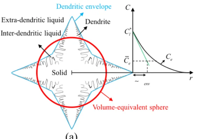
Following the pioneering work of Wang and Beckermann [5-9], to develop a macroscopic model for equiaxed solidification in an undercooled melt, a solidifying system is first assumed to consist of three phases: solid, inter-dendritic liquid, and extra-dendritic liquid. The two liquid phases are separated by the grain envelope, which is a virtual and smooth surface that connects the primary tips and the tips of actively growing secondary arms. A secondary arm is defined as active when it is longer than the next active secondary arm closer to the primary tip. Two liquid phases are introduced in the model because the solute diffusion is governed by length scales of different orders of magnitude: the secondary arm spacing in the inter-dendritic liquid and the distance between grains in the extra-dendritic liquid. Figure 1 shows a schematic of a grain envelope and the regions of the solid, inter-dendritic liquid, and extra-dendritic liquid phases, denoted by s, d, and e, respectively. Writing the local (i.e., the microscopic level) equation for the mass conservation in the extra-dendritic liquid in the absence of melt convection and solid motion, and using the averaging theorems discussed in detail in Wang and Beckermann [5] to average that equation over the volume of the REV, V0, results in the following volume-averaged equation for
the average growth kinetics:
0
1
env
env
env env env A
dg
dA S w
6
where genv, Aenv, wen v, n, Senv, and wenv are the envelope volume fraction (i.e., grain fraction),
envelope surface area, local envelope growth velocity vector, unit vector normal to the envelope surface and pointing outside the envelope, envelope surface area per unit volume of the REV (i.e.,
0
env
A V ), and average envelope growth velocity, respectively. This equation indicates that the
envelope volume fraction genv will increase, in other words growth will continue, as long as wenv
is greater than zero. The terms on the left-hand and right-hand sides of the first equality represent the change in the mass inside the envelope and the net rate of mass exchange at the envelope surface.
Writing the local equation for the solute conservation in the extra-dendritic liquid and following a procedure similar to the one discussed above equation (1) gives the volume-averaged equation for the average solute diffusion rates from the dendrite envelopes as:
* * * 1 1 env env e l e e l env e l env l e R E V A R E V A env g D g C C dA dA C S C C t V w n V j n t (2) where ge 1 genv, Ce, * l
C , je, Dl and env are the extra-dendritic liquid fraction, average solute
concentration in the extra-dendritic liquid, equilibrium solute concentration in the liquid, solute diffusion flux in the extra-dendritic liquid, solute mass diffusivity in the liquid, and average diffusion length around the envelopes, respectively. Note that, on the right-hand side of the first equality, the negative and positive signs of the first and second terms, respectively, reflect the fact that the unit vector n is defined to be pointing outside the envelope. These terms represent the
microscopic solute transfer (from the inter-dendritic to extra-dendritic) at the envelope surface. The first term represents the solute transfer due to the growth of the envelope and can be simply substituted using the first equality in equation (1) (note that *
l
7
REV and be, therefore, taken outside the integral). The second term represents the solute transfer due to the solute diffusion; the integral in this term can be modeled as the product of the envelope specific surface area Senv and a mean diffusive flux at the envelope surface. This flux can be
assumed to be directly proportional to the driving force for diffusion, which is the difference between the solute concentration in the extra-dendritic liquid adjacent to the envelope and the average solute concentration in the extra-dendritic liquid (i.e., *
l e
C C ), and inversely proportional
to the average diffusion length around the envelopes env; envis a measure of how far the solute has diffused away from the envelope. To better understand the concept of diffusion length, one can look at Figure 1, where a schematic of the solute distribution in the extra-dendritic liquid ahead of the primary tips is shown. The green line in the plot shows the tangent to the profile at the primary tip. The tangent intersects with the horizontal dashed line representing Ce , at a distance that is proportional to the envelope diffusion length env. Finally, the term *
l e
C C is linked to the
average undercooling in the extra-dendritic liquid, which is the driving force for growth.
In equations (1) and (2), the variables Senv, wenv, and env need to be obtained from constitutive
relations. The next section discusses the procedure to derive these relations and also the assumptions that have been commonly used in the literature to derive the currently available constitutive relations.
2.2 Constitutive Relations
To obtain the constitutive relations for the envelope variables Senv, wenv, and env, the envelope is
first approximated by the volume-equivalent sphere, referred to as sphere hereafter. A schematic of the sphere is also shown in Figure 1. Then, the envelope variables are related to the sphere variables as follows.
8
2.2.1 Relating envelope variables to sphere variables
The envelope surface area per unit volume of the REV, Senv, is related to the sphere surface area
per unit volume of the REV, Ssp, directly from the definition of the envelope sphericity
sp env
S
S (3)
One should note that the sphericity is a purely geometrical variable (i.e., it depends solely on the geometry of the envelope). The sphericity of a sphere is equal to unity by definition, and any other shape has a sphericity less than unity (for example, the sphericity of an octahedron is 0.85 [17]).
To relate the average envelope velocity, wenv to the sphere growth velocity, wsp, one needs to
recognize that equation (1) holds for any shape; since the volume of an envelope and its sphere are equal, the time derivative of envelope volume fraction and sphere volume fraction will be equal and one can, therefore, write Sen vwen v S wsp sp. In this relation, Senv can be substituted from
equation (3) to give:
env sp
w w (4)
Next, the variation of during growth is discussed. Equiaxed growth starts from a spherical nucleus, which has 1 and, from equation (4), wen v wsp 1. As the spherical nucleus grows into
the undercooled melt surrounding it, its shape becomes unstable and relatively fast growth along the energetically favorable crystallographic directions, compared to growth along the other directions, gradually transitions the shape into a dendrite, which has 1and, again from
9
equation (4), wen v wsp 1. Therefore, during growth, and wen v wsp decrease from their initial value of unity.
In the current literature, there are no relations to predict the decrease in or wen v wsp during growth. Therefore, macroscopic models had to rely on pre-determined and constant values for and wen v wsp . For example, in the study of Martorano et al. [18], and wen v wsp have been assumed to be equal to unity during the entire growth period; in other words, it is assumed that grains retain their initial spherical shape. In the studies of Appolaire et al. [19] and of Ludwig and Wu [20, 21], is assumed to be equal to 0.85 (i.e., the sphericity of an octahedron) and wen v wsp is assumed to be equal to the sphericity. Disregarding the decrease in and wen v wsp during growth can be expected to result in inaccuracies in the macroscopic models. In fact, Rappaz and Thevoz [22], compared the cooling curves measured in the experiments with the ones predicted by their solute diffusion model and noticed that their model does not predict the recalescence very well. They attributed this partly to the fact that in their model, sphericity was assumed to be equal to unity during the entire growth. As another example, Wu et al. [23, 24] did columnar to equiaxed transition (CET) simulations with different values for sphericity and found that the CET position is highly sensitive to the sphericity value. Developing a relation to predict the decreases in and, therefore, in wen v wsp , during growth is one of the objectives of this study.
To relate env to the sphere diffusion length, s p, one needs to realize that the envelope diffusion length is determined by the diffusion field around the envelope. It is therefore, in general, a complicated function of the envelope shape, size and growth velocity and a relation between env and s p cannot be obtained from a simple and purely geometrical analysis, such as the one we did to obtain equation (4). Such a relation has never been proposed in the literature mainly because the complex nature of solute diffusion field around an envelope precludes one from finding an analytical relation for env. Macroscopic models, therefore, have simply assumed en v sp[5-9,
10
18, 25]. This assumption might have reasonable accuracy during the initial stages of growth, when the envelope is spherical; however, as the envelope becomes dendritic with growth, the assumption can be expected to become increasingly inaccurate. Developing a relation for env is another objective of this study.
2.2.2 Relations for Sphere Variables
In the previous section, the envelope variables were related to the sphere variables. In this section, the relations for the sphere variables are outlined first and then interesting limiting cases of the relation for sp are discussed.
The sphere surface area per unit volume of the REV, Ssp , is calculated from
2 2 3 0 4 4 3 4 3 sp sp env sp sp sp env nR nR g S V nR g R (5)
where n and Rsp are the effective number of grains and the sphere radius, respectively. Note that,
in this equation, the first equality simply follows from the definition of Ssp and the second equality
follows from the definition of genv (i.e., the ratio of the total envelope volume to the REV volume
0
V ) and the fact that the envelope volume is equal to the sphere volume. The sphere radius Rsp is
calculated from sp sp dR w dt (6)
Next, the model needs a relation for wsp. Currently, macroscopic models assume simple fixed
11
constant geometrical factor [7, 17-24]. In reality, wsp depends on the velocity of the primary and secondary tips, and on the envelope shape. Developing a relation for wsp that accounts for the
realistic evolving envelope shape is one of the objectives of the present study.
The sphere diffusion length s p is calculated from the relation developed by Martorano et al. [18]
2 1 2 2 3 2 3 3 2 2 3 1 Iv Iv f sp sp f sp sp R P e R sp sp f sp sp sp sp f f sp f sp sp sp sp sp sp R P e R sp f sp sp f sp sp sp f sp sp R R R R R R R R e R R R P e P e P e P e R P e R R P e R P e e R P e R R P e (7)
where P esp w Rsp sp Dl is the sphere growth Péclet number, Rf is the final grain radius, and
Iv is the Ivantsov function. This equation indicates that the diffusion length around a sphere
depends on the radius and growth velocity of the sphere and the final grain radius. A better insight into this dependence can be obtained by simplifying equation (7) in two interesting limiting cases: the high P esp limit and the high Rf limit (i.e., the single grain limit). This is discussed next.
In the high P esp limit,
1
sp f sp
Pe R R
e converges to zero and therefore, inside the curly brackets on
the right-hand-side of the equation, the first three terms and the seventh term can be dropped; the fifth term becomes negligible compared to the fourth term; and, finally, in the last term, Iv Pesp
can be approximated by 1 1 P esp [26]. Therefore, equation (7) simplifies to
1
sp
sp sp
12
Interestingly, equation (8) indicates that in in the high P esp limit, s p does not depend on Rf . Using the definition of P esp, equation (8) can be recast into
l sp
sp
D
w (9)
The second interesting limiting case of equation (7) is the high Rf limit. In this limit, similar to
the high P esp limit discussed above,
1
sp f sp
Pe R R
e converges to zero. Therefore, inside the curly
brackets, the first three terms and the seventh term can be dropped; the fourth and fifth terms become negligible compared to the sixth term; finally, in the denominator of the term outside the curly brackets, 3
sp
R becomes negligible compared to R3f ; therefore, equation (7) reduces to
1 Iv sp sp sp P e R (10)
Note that the high P esp limit of this equation is, as expected, identical to the high P esp limit of equation (7) (i.e., equation (8)). In the low P esplimit, one has Iv Pesp 0[18] and equation (10) reduces to
sp Rsp (11)
2.2.3 Primary Tip Velocity
Macroscopic models need to predict the primary tip velocity, Vt , referred to as the tip velocity hereafter, because the growth of an envelope, at least during the early stages, is mainly driven by the growth of its primary arms. Therefore, the tip velocity, Vt can be expected to be one of the
13
main, if not the main factor, in determining wsp . In addition, Vt is required in predicting the primary arm length lt from
t t
dl V
dt (12)
To understand the variations of Vt during the quasi-steady growth of an assembly of dendrites,
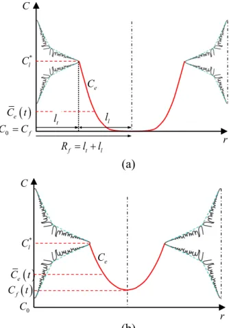
let us first consider two dendrites located at the distance 2Rf from each other inside a uniformly
undercooled melt, as shown schematically in Figure 2 at (a) an early time and (b) a late time during growth. Due to the symmetry, only half of the dendrites are shown. The profiles of solute concentration in the extra-dendritic liquid are also shown in the figure. Note that the concentration at the tip is equal to the equilibrium concentration *
l
C and it decreases as one moves away from
the tip towards the liquid. At the early time (i.e., Figure 2(a)), this decrease continues until some distance ahead of the tip, where the concentration reaches the initial solute concentration C0 and
remains constant after that; therefore, the concentration at the symmetry line between the grains f
C is equal to C0: Cf C0; at the late time (i.e., Figure 2(b)), the decrease continues through the
entire liquid region up to the symmetry line between the two grains, where the concentration reaches Cf , which has a value greater than C0: Cf C0.
At the early stage of growth, shown in Figure 2(a), there is a distance between the edges of the solutal boundary layers ahead of the tips and, therefore, the solutal field ahead of one dendrite is not influenced by the presence of the other. In other words, the dendrites are not interacting. This stage of growth is, therefore, referred to as the non-interacting stage. At this stage, the growth of the dendrites is virtually the same as the growth of a single dendrite into an essentially infinite medium. As the dendrites keep growing, the distance between the edges of the boundary layers decreases and at some intermediate time the edges meet. Once that happens, the solutal boundary layer ahead of each of the dendrites starts to get influenced by the presence of the other dendrite.
14
In other words, the dendrites start to interact. This stage is called the interacting stage. Next, the variations of Ce and Cf during these two stages and the relationships between them and C0 are
discussed. During the non-interacting stage, Cf remains constant and equal to C0 ; furthermore,
f
C is less than the average solute concentration in the extra-dendritic liquid Ce t :
0 f e
C C C t . During the interacting stage, however, Cf is greater than C0 but still less than
e
C t : C0 Cf Ce t . These two relations are important, and will be referred to subsequently when the time variations of Vt during these two stages is discussed.
As the primary arm of a dendrite grows, it rejects solute (assuming k0 1). For growth to continue, the rejected solute needs to be dissipated away from the tip towards the bulk liquid. The balance between the solute flux rejected at the tip and the solute flux diffusing away from the tip determines the tip velocity. The latter flux is proportional to the solute gradient at the tip. During the non-interacting stage of growth, the diffusion field ahead of the tip and therefore the diffusion flux at the tip remain constant. This causes Vt to remain constant. During the interacting stage, however,
f
C increases with time, which makes the solute profiles progressively smoother; therefore, the
solute diffusion flux at the tip and consequently Vt both decrease with time. Prediction of Vt during these stages is discussed next.
In macroscopic models of solidification, the most commonly used relation for predicting Vt is the relation proposed by Ivantsov [27]:
, exp E1
t eff P et P et P et (13)
where t eff, is an effective tip undercooling (i.e., the undercooling corresponding to the effective
far-field solute concentration, which should not be confused with the solute concentration at the symmetry line between two adjacent grains Cf discussed earlier in connection with Figure 2) and
15 2
t t t l
P e V R D is the dendrite tip Péclet number, Rt d D0 l Vt is the tip radius, k0 is
the partition coefficient, d0 is the capillary length, is the tip selection parameter, and the
function E1 is the exponential integral function. Equation (13) is the exact similarity solution for the solute diffusion field around a paraboloid of revolution during its quasi-steady shape-preserving growth into an infinite medium with uniform and constant far-field undercooling t eff,
. This equation has been shown to provide accurate predictions of the primary tip velocity Vt
during the quasi-steady growth of a single dendrite into an essentially infinite medium [28]. For the quasi-steady growth of multiple dendrites, equation (13) can be expected to accurately predict
t
V during the non-interacting stage. To predict Vt during the interacting stage, modifications to
this equation have been proposed [29, 30]. These modifications are, however, limited to isothermal dendrites and specific dendritic arrangements and a generally valid relation to predict Vt during the interacting stage is still not available. Therefore, similar to the numerous studies in the literature [5, 7, 8, 18, 31], in this paper, equation (13) is used to predict Vt during both non-interacting and interacting stages.
In using equation (13) to predict Vt during the growth of multiple dendrites one should keep in mind that, as depicted in Figure 2 and discussed in the figure discussion, during both the interacting and non-interacting stages, one has Cf Ce; since the effective far-field solute concentration is equal to and less than Cf during the non-interacting and interacting stages, respectively, the effective tip undercooling t eff, will be always higher than the average undercooling in the extra-dendritic liquid e , which is defined as
* * 0 1 l e e l C C k C (14)
16
In other words, during the entire growth period, one has e t eff, . Therefore, if, in equation (13),
e is used instead of t eff, , the tip velocity Vt will be underpredicted. Using e in this equation has been, however, a common practice in the literature [5, 7, 8] because, currently, there are no relations to predict t eff, . Developing a relation to predict t eff, is one of the objectives of this study.
3 Mesoscopic Envelope Model
The mesoscopic envelope model used in the present study was originally developed by Delaleau [14] and recently used by Souhar et al. [15] to perform three-dimensional simulations of equiaxed growth. The reader is referred to these papers for the details of the model and the complete set of equations. In brief, the model approximates the complex dendritic structure with an envelope and a solid fraction field inside the envelope. The normal growth velocity at any point on the envelope is calculated from the local dendrite tip velocity, obtained from an analytical stagnant film model, and the angle between the growing dendrite arm and the envelope normal. The stagnant film model gives the tip local velocity as a function of the undercooling of the liquid in the vicinity of the envelope. The envelope growth and the solute transport in the liquid around the envelope are thus coupled. The liquid inside the envelope and on the envelope surface is assumed to be well-mixed and in equilibrium with the solid while the liquid outside the envelope is generally undercooled. The solid fraction field inside the envelope and the solute concentration field in the extra-dendritic liquid outside the envelope Ce are obtained from the numerical solution of a solute conservation
equation that is valid both inside and outside the envelope. Hence, the solutal interactions between the growing grains are fully resolved.
17
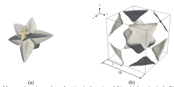
The first set of mesoscopic simulations were performed for the isothermal growth of a single grain growing into an essentially infinite domain (Figure 3(a)) and for multiple grains (Figure 3(b)) with high/low grain densities of Rf D Vl Iv 0 = 4.03/6.31, where VIv 0 is the Ivantsov tip velocity (i.e., the velocity predicted by equation (13)) corresponding to the initial undercooling
0. Each case was simulated for 0 0.05 and 0.15. For the multiple grain cases, the grains were
arranged periodically in a BCC lattice, with the primary arms growing along the axes (Figure 3(b)).
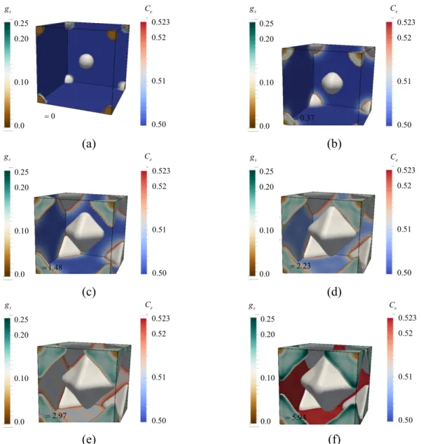
In Figure (4), an example of the mesoscopic simulation results is shown. The figure, which is for the multiple grain case with the low undercooling ( ) and high grain density (
0 4.03
f l Iv
R D V ), shows the solid fraction, gs, and the solute concentration in the
extra-dendritic liquid Ce, plotted in the interior and exterior of the envelopes, respectively, at different
times. The dimensionless time, , is scaled by the time needed for a steady-state tip to advance by one diffusion length: VIv 0 D Vl Iv 0 . It can be seen that, as expected (see the discussion
below Equation (4)), the envelope is initially spherical (see Figure 4(a)), but it gradually becomes dendritic during growth. It can also be seen that during the growth, the envelopes reject solute to the extra-dendritic liquid and, therefore, Ce increases. At the early times (i.e., 0.37), this
increase is limited to a relatively small distance ahead of the envelopes; therefore, Ce further away
from the envelopes is still at the initial value of 0.5 wt. pct.. At the later times (i.e., 2.23), Ce
everywhere in the domain has become greater than 0.5. Finally, at 5.94, Ce everywhere has
reached the equilibrium solute concentration *
0.523
l
C ; the undercooling has fully vanished and
the growth has ended.
Another example of the mesoscopic simulation results is shown in Figure 5. The figure, which, similar to Figure 4, is for the multiple grain case with the low undercooling and high grain density, shows the final envelope shape and the profiles of solute concentration in liquid along the line connecting the primary arms of two dendrites growing towards each other. Different curves show
18
the profiles at different times. From the plot it can be seen that at 2.6 the solutal fields ahead of the grain envelopes overlap and, therefore, the grains start interacting.
3.2 Upscaling Mesoscopic Results
To upscale the mesoscopic simulations results, they were averaged over the volume of the REV. For example, at any time during growth, the solute concentration field in the extra-dendritic liquid was averaged over the volume of the REV to give the value of Ce at that time. In Figure 6, the upscaled mesoscopic results are plotted as a function of the non-dimensional time defined as
2 0
Iv l
tV D . Results for a single grain are shown as black curves and for multiple grains with
high and low grain density as red and blue curves, respectively. Results for and 0.15 are plotted as solid and dashed curves, respectively.
Figure 6(a) shows the envelope volume fraction genv. Squares in the figure represent the start of
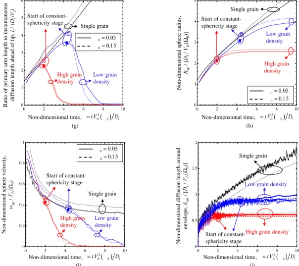
the second stage of growth and the definitions of the first and second stages will become clear subsequently, when Figure 6(g) is discussed. Figure 6(b) shows the non-dimensional average undercooling in the extra-dendritic liquid e 0 , where e was calculated from equation (14). Figure 6(c) and Figure 6(d), a close-up of 6(c) around 5, show the sphericity, which was calculated using equation (3) after calculating Senv and Ssp as follows: Senv was measured directly from the simulated envelope shape, and Ssp was calculated from equation (5), after computing Rsp from an equation that is derived subsequently in connection with Figure 6(h). Figure 6(e) shows the non-dimensional primary arm length lt D Vl Iv 0 , where lt was measured directly from
the simulated envelope shape. Figure 6(f) shows the non-dimensional tip velocity V Vt Iv 0 , where Vt was calculated from equation (12). Figure 6(g) shows the scaled primary arm length lt* defined as
19 * t t diff l l l (15)
where ldiff is the instantaneous diffusion length ahead of the primary tip, which is defined as
l diff t D l V (16)
Figure 6(h) shows the non-dimensional sphere radius Rsp D Vl Iv 0 . The sphere radius, Rsp ,
is calculated using an equation that relates Rsp to the final grain radus Rf , to the envelope fraction, env
g , and to the effective number of grains inside the REV, n. In what follows, this equation is
first derived using a formal procedure, to show that the equation is the integrated form of equation (1). Next, it is discussed that the equation can be written directly from the definition of the sphere. The formal derivation of the equation starts with first substituting the right-hand side of equation (1) using Sen vwen v S wsp sp (see the discussion above equation (4)); then, Ssp and wsp are substituted from equations (5) and (6), respectively, to give
sp env env sp dR dg dt g dt R dt 1 3 (17)
Next, the definite integrals of both sides of this equation are taken from time zero to time t to give
sp env env sp R g g t R t 3 0 0 (18)
In this equation, genv t 0 and Rsp t 0 are the envelope fraction and sphere radius corresponding to the initial spherical seeds. Since the initial seeds have the same size, genv t 0 and Rsp t 0 can be related as
1 3 1 3
0 2 3 4 0
sp f env
20
number of grains inside the REV, which is equal to unity for a single grain and two for multiple grains in the BCC arrangement. Substituting this equation into equation (18) gives
1 3 1 3 3 2 4 sp f env R R g n (19)
Note that this equation has a simple physical meaning: it indicates that, as expected, at any time during growth, the total volume of the spheres (i.e., 3
4 sp 3
n R ) is equal to the total volume of
the envelopes (i.e., 3
8R gf env). In fact, one can write this equation directly from the definition of the
sphere. Here, however, the more formal procedure to derive it is provided to show that equation (19) is indeed the integrated form of equation (1).
Figure 6(i) shows the non-dimensional sphere velocity wsp VIv 0 , where wsp was calculated from equation (6). Figure 6(j) shows the non-dimensional average diffusion length around the envelopes env D Vl Iv 0 , where env was determined from equation (2) by solving this
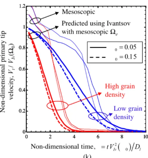
equation for env, using the upscaled mesoscopic values for all the other quantities. Finally, Figure 7 shows the comparison between the mesoscopic primary tip velocities and the Ivantsov tip velocities corresponding to e. Next, the important observations that can be made from these plots are discussed.
From Figures 6(a) and 6(b) it can be seen that for a single grain genv and e remain close to zero and 0, respectively, during the entire growth. This is because for the single grain cases the size of the simulation domain was chosen to be large enough to remain much larger than the envelope size during the entire growth. For the multigrain cases, however, the envelope fraction increase relatively fast initially because e, which is the driving force for growth, is relatively high; as e decreases, due to the solute rejection from the envelopes to the extra-dendritic liquid, the rate of
21
increase in genv decreases. Finally, when the undercooling is fully consumed (at about 4 and 9
for the high and low grain density cases, respectively) genv ceases to increase further and growth
ends.
From Figures 6(c) and 6(d) it can be seen that, as expected, the initial value of is equal to unity and as the envelope becomes progressively more dendritic with growth, decreases. For a single grain, this decrease continues until 40. At this time, we stopped the simulations because the diffusion field around the envelope started to interact with the boundaries of the simulation domain. For the multigrain cases, however, after a relatively small initial decrease (of about 0.1 for the high grain density cases and 0.2 for the low grain density cases) stops to decrease further and then remains constant.
From Figure 6(f) it can be seen that at an early stage of growth ( less than two) we have 0
1 Vt VIv : the mesoscopic tip velocities Vt are greater than the Ivantsov tip velocities
corresponding to the initial undercooling VIv 0 . This is because of the presence of an initial transient stage in the mesoscopic simulations, where the Ce field is transitioning from the initial
value of Ce C0 (see Figure 6(a)) to the quasi-steady values. During this stage, the solutal gradient
ahead of the tip and therefore the tip velocity is greater than the quasi-steady values predicted by equation (13).
At the end of the initial transient stage ( about 2), the quasi-steady stage starts. During this stage, t
V for a single grain (i.e. the black curves) remains, as expected, constant, but at a value that is
slightly (about 10 percent) lower than the Ivantsov tip velocity corresponding to the initial undercooling 0. This minor underprediction of the tip velocities by the mesoscopic model is of no significant consequence and should not distract; however, for the sake of completeness, the reason for it is explained next. As already discussed in detail by Steinbach et al. [1, 2] and Souhar
22
et al. [15, 32], in the mesoscopic model, the predicted tip velocities depend on a parameter in the model known as the stagnant film thickness f . For the high values of f (i.e. f 3ld iff [15, 32]) the mesoscopic tip velocity for a single grain will be equal to the Ivantsov tip velocity. However, with such a high value of f , the predicted grain envelope shapes will be unrealistic (compared to the experimentally observed ones [16]). Therefore, to have relatively accurate predictions for both Vt and the envelope shape, a compromising intermediate value for f needs to be chosen. As a result of this compromise, the quasi-steady mesoscopic tip velocities are slightly lower than the Ivantsov tip velocities.
The tip velocity Vt for the multiple grain cases starts to rapidly decrease at some intermediate time (about = 2 for the high grain density cases and 4.5 for the low grain density cases). This rapid decrease is physically important and indicates that the tips are solutally interacting.
From Figure 6(g) it can be seen that *
t
l , which was defined in equation (15), for single grain cases
increases with time during the entire growth period. For the multigrain cases, however, *
t
l increases
with time initially, but, at some intermediate time which is denoted by the squares in the figure, *
t
l
starts to decrease with time and eventually reaches zero (since ld iff as the result of Vt 0). Therefore, the entire growth period can be divided into two stages: the first stage, where *
0
t
d l d t
, and the second stage, where *
0
t
d l d t . These two stages should not be confused with the
interacting and interacting stages discussed in connection with Figure 2. The interacting and non-interacting stages concerned the growth of the primary arms, while the first and second stages introduced here concern the average growth kinetics of the envelopes. It will be shown below that the first and second stages can be referred to as variable-sphericity and constant-sphericity stages, respectively. Dividing the entire growth period into variable-sphericity and constant-sphericity stages based on the sign of *
t
d l is an important premise that is proposed in this study and will be
23 Variations of *
t
l during these two stages can be understood by following the variations of lt and
t
V , shown in Figures 6(e) and 6(f), respectively, and focusing on how the nominator and
denominator of equation (15) change with time. During the first stage, Vt is relatively high (i.e.,
greater than 0.8 VIv 0 ) and therefore, lt, which appears in the nominator of equation (15), increases relatively fast; this causes *
t
l to increase with time during the first stage. When the second
stage starts, Vt has an intermediate value and, more importantly, is decreasing fast. Therefore,
unlike in the first stage, the increase in lt is not fast anymore and becomes insignificant compared to the fast increase in ldiff , which appears in the denominator of equation (15); this causes,
*
t
l to
decrease with time during the second stage.
There is one last interesting point about Figure 6(c) that can be discussed now because the first and second stages of growth were defined. It can be seen from this figure that the variations of the sphericity during the second stage of growth (i.e., the right-hand side of the squares) are negligible compared to these variations during the first stage of growth and, therefore, the sphericity can be assumed to be constant during the second stage of growth. Consequently, in the rest of the paper, the first and second stages of growth are referred to as variable-sphericity and constant-sphericity stages, respectively.
Figure 6(i) shows the time variations of the non-dimensional sphere velocity. From the figure, it can be seen that during the variable-sphericity stage of growth (i.e., the left-hand side of the squares), the multigrain curves collapse on the single grain curves. This indicates that during the variable-sphericity stage of growth, wsp for multigrain and single grain cases can be expected to
be predicted by the same relation. When the constant-sphericity stage starts, however, the multigrain curves cease to collapse on the single grain curves, and they start decreasing relatively
24
rapidly. This indicates that wsp during the constant-sphericity stage of growth needs to be predicted
from a separate relation.
Comparing the time variations of Vt, shown in Figure 6(f), and time variations of wsp, shown in
Figure 6(i), reveals another interesting observation. Focusing first on the low grain density cases (the blue curves), one can see that at 8, Vt is zero: the primary tips have fully stopped. At the
same time, however, wsp is still greater than zero: the envelopes are still growing. This indicates
that growth continues (at least until 10) even after the primary tips stop. A similar trend is observed for the low grain density curves. Growth of an envelope after the primary tips stop is due to the growth of the secondary arms.
In Figure 7, the mesoscopic primary tip velocities (the thin curves) are compared with the Ivantsov tip velocities, predicted using equation (13) with t eff, e (the thick curves). Data are shown only for the multigrain cases. One can see from the figure that, as expected (see the discussion below equation (14)), setting t eff, e in the Ivantsov solution significantly underpredicts the tip velocities.
Finally, this section is ended by summarizing the important observations that can be made from the upscaled mesoscopic results: 1) for the multiple grain cases, the entire growth period can be divided into the variable-sphericity and constant-sphericity stages and these two stages correspond to the positive and negative values of *
t
d l , respectively; 2) for the single grain cases, the growth
takes place entirely in the first stage; 3) setting t eff, e in the Ivantsov relation will significantly underpredict the tip velocities.
25 4.1 Postulates
It is postulated that during the variable-sphericity stage of growth, is a function of lt Rsp only and during the constant-sphericity stage of growth, is, obviously, constant.
* * 0 0 0 t t sp t l dl R dl d (20)
It is known from the literature [27] that the shape of a dendrite depends on the surface tension anisotropy; therefore, one might wonder why such a dependence is not introduced in equation (20). This is because in this equation (and through the entire paper) is the sphericity of the dendrite envelope and, therefore, depends on the envelope shape (which shall not be confused with the dendrite shape). From what is available in the literature, it is not clear whether the envelope shape depends on the surface tension anisotropy or not. What is known from the literature is that the envelope shape, and therefore, the sphericity predicted by the mesoscopic model, has been validated against experiments of equiaxed solidification of SCN-acetone [1,15] and of directional solidification of Al-Cu [14]. Since, as will be shown in section 5, the mesoscopic values of are accurately predicted by taking the sphericity as a function of lt Rsp only, introducing surface tension anisotropy effects in equation (20) does not seem to be necessary.
To develop a relation for wsp, one first needs to recognize that the average growth kinetics, and
therefore wsp, are in general determined by the growth of both the primary and the secondary arms.
At early stages of growth, the primary arms grow much faster than the secondary arms. Therefore, their velocity can be expected to be the main factor in determining wsp. As the growth continues,
the primary arms slow down and finally stop, but the secondary arms and therefore the sphere continue to grow, until the undercooling in the extra-dendritic liquid fully vanishes (i.e., the
26
average undercooling in the extra-dendritic liquid reaches zero). In other words, at some intermediate time during growth, the main mechanism that drives the envelope growth, and thus determines wsp, transitions from the primary tip velocity to the average undercooling of the
extra-dendritic liquid. This transition and the time at which it occurs need to be properly taken into account in developing the relation for wsp. In this paper, it is first postulated that the transition
occurs when the constant-sphericity stage of growth starts. The postulates to determine wsp during
the variable-sphericity and constant-sphericity stages are discussed next.
During the variable-sphericity stage, wsp is assumed to scale with the primary tip velocity Vt. It
should be noted that wsp Vt cannot be taken as constant because the shape of the envelope changes significantly during the variable-sphericity stage. In the macroscopic model, the envelope shape is represented solely by the envelope sphericity . In other words, is assumed to contain all the geometrical information about the envelope shape. Since itself is postulated to be a function of
t sp
l R only (see equation (20)), wsp Vt is similarly postulated to be a function of lt Rsp only.
During the constant-sphericity stage, wsp is assumed to scale with wsp ts , where ts is the time at
the start of the constant-sphericity stage, and the ratio wsp wsp ts is postulated to be a function
of the scaled Ivantsov velocity corresponding to e, VIv e VIv e ts , only. The above three postulates can be expressed mathematically as
* * 0 0 sp sp t t t t sp sp sp Iv e t sp s sp s Iv e s w w l dl V V R w w V dl w t w t V t (21)
27
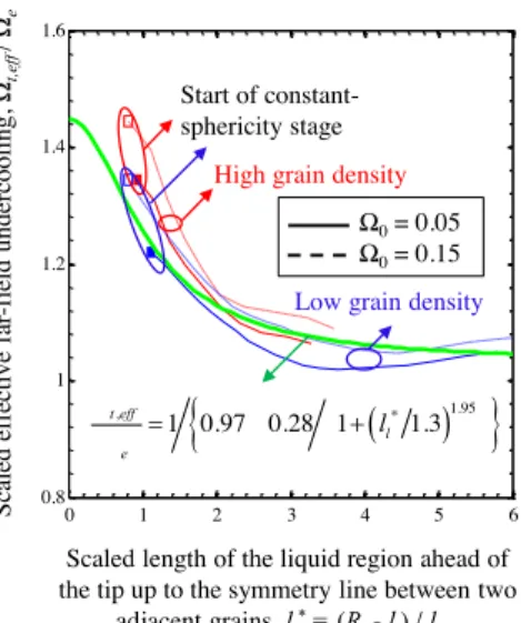
Through the entire growth period, t eff, is assumed to scale with e, and the ratio t eff, e is assumed to be a function of the scaled length of the free liquid region ahead of the primary tip up to the symmetry line between two adjacent grains * * *
l f t l R l , where R*f Rf ldiff : , , * t eff t eff l e e l (22)
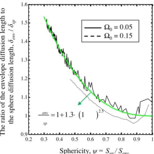
The envelope diffusion length, en v, is assumed to scale with the sphere diffusion length, sp (Eq. (7)), and the ratio env sp is assumed to be a function of sphericity only:
env env
sp sp
(23)
Note that env sp could have been formulated as a function of lt Rsp instead of , because is a function of lt Rsp only (see equation (18)) but here it is formulated as a function of the
envelope sphericity to better illustrate that the ratio of the envelope diffusion length to the sphere diffusion length is a function of the envelope geometry, which is represented by the envelope sphericity.
4.2 Fitting Functions
In this section, the upscale mesoscopic results, presented in section 3.2, are used to plot the left-hand-side of equations (20) to (23) as a function of the independent variable on the right-hand-side. The constitutive relations are then developed by curve fitting these plots. In the following figures, mesoscopic results for a single grain are shown as black curves and for multiple grains with high and low grain density as red and blue curves, respectively. Results for and
28
0.15 are plotted as solid and dashed curves, respectively; the green curves depict our curve fits and the squares show the start of the constant-sphericity stage of growth.
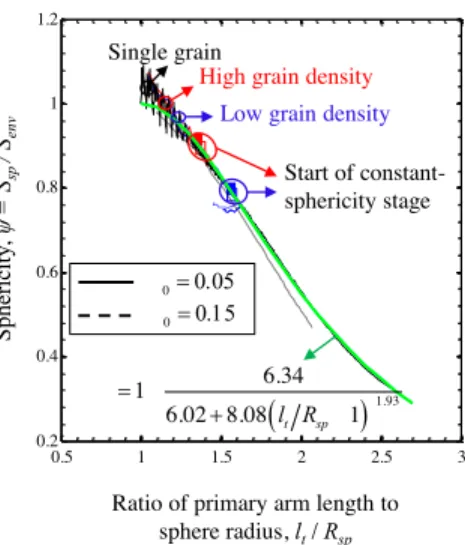
In Figure 8, the sphericity is plotted as a function of the ratio of the primary dendrite arm length to the sphere radius lt Rsp . It can be seen that for a single grain, the mesoscopic simulation results for the two different initial undercoolings 0 collapse onto a single curve. This indicates that the
sphericity is indeed a function of lt Rsp only. The multigrain data in the plot fall on the same curve as the single grain data during the variable-sphericity stage of growth. However, when the constant-sphericity stage starts, the multigrain data start to deviate slightly from the sphericity curve for a single grain. The variation of during this stage are, however, extremely small and are disregarded. The final fit of the sphericity data for both the single grain and the multigrain cases is then given by:
* 1.93 * 6.34 0 1 8.08 6.02 1 0 0 t t sp t dl l R dl d (24)
This equality can be understood as follows. Initially (i.e., 0), the envelope is spherical and t sp
l R is equal to unity; therefore the denominator on the right-hand side will be large, which will
make the sphericity become equal to unity. During growth, as the envelope shape transitions from a spherical to a dendritic, lt Rsp increases; the second term on the right-hand-side increases, and
therefore decreases.
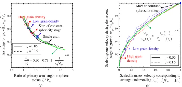
In Figure 9(a), wsp Vt during the variable-sphericity stage of growth is plotted as a function of
t sp
l R . It can be seen that wsp Vt decreases monotonically as lt Rsp increases. Since the single
29
the variable-sphericity stage of growth is indeed a function of lt Rsp only, and can be fit by
0.85
0.80 0.78 1 1
sp t t sp
w V l R . In Figure 9(b), wsp wsp ts is plotted as a function of Iv e Iv e s
V V t . Single grain data cannot be included in this plot because, as discussed in
connection with Figure 6(g), for a single grain growth takes place solely at the variable-sphericity stage. One can see that the multigrain data for the two different initial undercoolings 0 collapse
onto a single curve. This indicates thatwsp wsp s is indeed a function of VIv e VIv e s only. The final fit for wsp wsp s is then given by
0.50
sp sp s Iv e Iv e s
w w t V V t .
Summarizing the fits proposed in Figures 9(a) and 9(b), we get
0.85 * 0.50 * 1 0 0.80 0.78 1 0 sp t t t sp sp Iv e t sp s Iv e s w d l V l R w V d l w t V t (25)
In Figure 10, the scaled effective far-field undercooling t eff, e is plotted as a function of *
l
l ;
,
t eff was calculated from Equation (13), together with the relation for the tip radius (see the discussion below Equation (13)), using the mesoscopic values for Vt . Note that t eff, is an
effective undercooling that is to be used in the Ivantsov relation (Eq. (13)) in order to obtain accurate tip velocities for the primary tips of interacting dendrites. Data is shown only during the variable-sphericity stage of growth because the curves for the different mesoscopic cases did not collapse during the constant-sphericity stage of growth. This, however, should not distract because, as will become clear at the end of this section, in the macroscopic model, the calculation of Vt and
therefore t eff, are not required during the constant-sphericity stage. Variations of t eff, e with
*
l
l can be best understood by first focusing on the data for the high undercooling low grain density
case (i.e., the dashed blue curve). Initially (i.e., at 0), *
l
l has its highest value (about six) and
,
30
and due to the presence of the initial transient stage, Vt is initially greater than VIv 0 . During growth, lt increases and therefore
*
l
l decreases. For ll* 2, t eff, e remains almost constant because the rate of decrease in t eff, and e are almost the same; however, at
*
l
l about two,
,
t eff e starts to increase because the rate of decrease in e starts to become greater than the rate of decrease in t eff, . The curves for the other mesoscopic cases behave in a similar fashion and,
despite the minor spread between them, they can be fit by a single curve given by
, 1.95 * 1 0.28 0.97 1 1.3 t eff e l l (26)
There are two more points about Figure 10 and equation (26) that need to be discussed before pursuing. First, focusing on the blue curves in the figure, it can be seen that they do not collapse fully and have a minor spread. This minor spread causes imperfections in the fit for f e and is attributed to the presence of an initial transient stage in the mesoscopic simulations. The collapse between these curves cannot reasonably be expected to be better because, as was shown in Figure 6(f), the curves representing Vt for the mesoscopic cases with different initial undercoolings did
not collapse during the initial transient stage. Similarly, the collapse between the red curves in Figure 10 cannot be expected to be better. Second, the first term in the denominator of the right-hand-side is chosen to be slightly less than unity. In this way, for free growth of a single grain and at the early stages of multigrain growth, where the second term in the denominator is almost zero because *
l
l is high, t eff, becomes slightly higher than e ( t eff, 1.031 e). Therefore, initially (i.e., at 0), the predicted tip velocity Vt will be higher than VIv 0 . This means that the macroscopic model can predict the initial transient effects on the tip velocity. However, since the stagnant-film model used to calculate the tip velocity in the mesoscopic model is based on the assumption of a steady-state diffusion field within the stagnant film, the tip velocities predicted by the macroscopic model during the initial transient stage can only be expected to be approximate.
31
In Figure 11, env sp for the single grain cases is plotted as a function of . It can be seen that as decreases during growth, env sp increases monotonically above unity. This indicates that the diffusion length around a complex shaped dendritic envelope is greater than the diffusion length for the sphere. Since the data for the two different initial undercoolings collapse, env sp is indeed a function of only. A curve fit to the data for the single grain is given by:
2.5
1 1.3 1
env
sp
(27)
In summary, the macroscopic model consists of equations (1) to (7), (12) to (16), and (24) to (27). It requires two inputs: the initial undercooling 0 and the final grain radius Rf . Also, note that lt and Vt appear only in the first relation of equations (24) and (25), respectively. Therefore, the
model needs to calculate Vt during the variable-sphericity stage only.
5 Comparing the Macroscopic Predictions with the Upscaled Mesoscopic Results
In this section, the constitutive relations are verified by comparing the predictions of the macroscopic model against the upscaled mesoscopic results. It is pointed out that the individual constitutive relations that were each separately fitted to the upscaled mesoscopic simulations are now used in conjunction in a closed macroscopic model. The comparisons are first made for the isothermal mesoscopic cases, presented in section 3.2, and used in section 4 to develop the constitutive relations. Next, to provide further confidence in the constitutive relations, comparisons are made against new upscaled mesoscopic results that are representative for conditions in solidification processing of metal alloys.
32 5.1 Isothermal Cases
Figures 12 and 13 show the comparisons between the predictions of the macroscopic model for different quantities (the thick curves) with the corresponding upscaled mesoscopic results (the thin curves) for the four isothermal cases. Figure 12 shows the comparisons for the low grain density cases with the low/high undercoolings (the solid/dashed curves) and Figure 13 shows the similar comparison for the high grain density cases. For all the four cases, the overall agreements between the macroscopic predictions and the upscaled mesoscopic results are good and, as is discussed next, cannot realistically be expected to be much better.
In Figures 12(e) and 13(e) the tip velocities predicted by the macroscopic model are compared with the mesoscopic tip velocities. Note that, as discussed at the end of section 4, in the macroscopic model the tip velocities need to be predicted only during the variable-sphericity stage. Plotting the tip velocities during the constant-sphericity stage for the isothermal cases is only because, for these cases, the mesoscopic and macroscopic predictions of the tip velocity were in good agreement. It can be seen that, during the entire growth period, the predicted tip velocities agree reasonably well with the mesoscopic tip velocities. Contrasting this agreement with the vast difference that was observed in Figure 7 between the mesoscopic tip velocities and the Ivantsov velocities corresponding to e, one can easily acknowledge that the tip velocities predicted by our model (i.e., the Ivantsov velocities corresponding to t eff, ) are, as expected, significantly more
accurate (when compared against the mesoscopic tip velocities) than the Ivantsov velocities corresponding to e.
The minor difference between the macroscopic and mesoscopic tip velocities is attributed to the presence of the initial transient stage in the mesoscopic simulations, which, as discussed in connection with Figure 10, causes imperfections in our fit for t eff, e .
33
Before proceeding, it is necessary to iterate that the constitutive relations developed in this paper are based only on the upscaled mesoscopic results for a single grain growing into an essentially infinite medium as well as multiple grains with the periodic arrangement. In reality, however, grains can have a random arrangement. Therefore, a necessary future work is to examine the agreement between the predictions of the macroscopic model and the upscaled mesoscopic results for multiple grains with a random arrangement. If this agreement is found to be not as good as the agreement that was achieved in Figures 12 and 13, then the constitutive relations will need to be improved. We, however, expect that the predictions of the relation for (i.e., equation (24)), and the relation for wsp during the variable-sphericity stage of growth (i.e., the first equality in equation
(25)), will be still in a good agreement with the corresponding mesoscopic results for multiple grains with random arrangment. This is because, for and wspduring the variable-sphericity
stage, the mesoscopic data for multiple grains with BCC arrangement collapsed on the data for a single grain (see Figure (8) and 9(a)); therefore, it can be expected that data for multiple grains with random arrangement will also collapse on the single grain data. As a result, it is expected that the fit in Figure 8, and therefore the relation for , and also the fit in Figure 9(a), and therefore the relation for wsp during the variable-sphericity stage of growth, will remain unchanged even if
mesoscopic data for multiple grains with random arrangement is added to Figure 8 and Figure 9(a). The agreements between the predictions of the relations for wsp during the constant-sphericity
stage of growth, t eff, and env with the corresponding mesoscopic values might not be as good as the agreement observed in Figures 12 and 13. If that turns out to be the case, these relations will need to be improved, and this is a necessary future work.
5.2 Recalescence Cases
To further verify the constitutive relations, new mesoscopic simulations were performed and the predictions of the macroscopic model were compared with the upscaled mesoscopic results. These