Learning to Detect Motion Boundaries

HAL Id: hal-01142653

https://hal.inria.fr/hal-01142653

Submitted on 15 Apr 2015

HAL is a multi-disciplinary open access

archive for the deposit and dissemination of

sci-entific research documents, whether they are

pub-lished or not. The documents may come from

teaching and research institutions in France or

abroad, or from public or private research centers.

L’archive ouverte pluridisciplinaire HAL, est

destinée au dépôt et à la diffusion de documents

scientifiques de niveau recherche, publiés ou non,

émanant des établissements d’enseignement et de

recherche français ou étrangers, des laboratoires

publics ou privés.

Learning to Detect Motion Boundaries

Philippe Weinzaepfel, Jerome Revaud, Zaid Harchaoui, Cordelia Schmid

To cite this version:

Philippe Weinzaepfel, Jerome Revaud, Zaid Harchaoui, Cordelia Schmid. Learning to Detect Motion

Boundaries. CVPR - IEEE Conference on Computer Vision & Pattern Recognition, Jun 2015, Boston,

United States. pp.2578-2586, �10.1109/CVPR.2015.7298873�. �hal-01142653�

Learning to Detect Motion Boundaries

Philippe Weinzaepfel

Jerome Revaud

Zaid Harchaoui

Cordelia Schmid

a

_Inria

_NYU

firstname.lastname@inria.fr

Abstract

We propose a learning-based approach for motion boundary detection. Precise localization of motion bound-aries is essential for the success of optical flow estimation, as motion boundaries correspond to discontinuities of the optical flow field. The proposed approach allows to pre-dict motion boundaries, using a structured random forest trained on the ground-truth of the MPI-Sintel dataset. The random forest leverages several cues at the patch level, namely appearance (RGB color) and motion cues (optical flow estimated by state-of-the-art algorithms). Experimen-tal results show that the proposed approach is both robust and computationally efficient. It significantly outperforms state-of-the-art motion-difference approaches on the MPI-Sintel and Middlebury datasets. We compare the results ob-tained with several state-of-the-art optical flow approaches and study the impact of the different cues used in the ran-dom forest. Furthermore, we introduce a new dataset, the YouTube Motion Boundaries dataset (YMB), that com-prises60 sequences taken from real-world videos with man-ually annotated motion boundaries. On this dataset, our ap-proach, although trained on MPI-Sintel, also outperforms by a large margin state-of-the-art optical flow algorithms.

1. Introduction

Digital video content, such as home movies, films and surveillance videos, is increasing at an exponential rate. Au-tomated analysis of such video content requires fast and scalable approaches for many computer vision tasks, such as action and activity recognition [19, 34], video surveil-lance of crowds [15], sport video understanding [23]. All these latter approaches rely on optical flow. Therefore, de-signing a fast and precise optical flow estimation method is essential.

State-of-the-art methods for optical flow computation are usually cast into an energy minimization framework. Coarse-to-fine algorithms [6] are then used to efficiently

∗_{LEAR team, Inria Grenoble Rhone-Alpes, Laboratoire Jean}

Kuntz-mann, CNRS, Univ. Grenoble Alpes, France.

(a) Image (b) Ground-truth motion boundaries

(c) Flow gradient (Classic+NL) (d) Proposed method

Figure 1. For the image in (a), we show in (b) its ground-truth motion boundaries, in (c) motion boundaries computed as gradi-ent of the Classic+NL [28] flow, and in (d) the proposed motion boundary detection. Despite using the Classic+NL flow as one of our cues, our method is able to detect motion boundaries even at places where the flow estimation failed, such as on the spear or the character’s arm.

minimize the energy objective [2,9,28,33]. However, such approaches can be sensitive to initialization. Therefore, the prior information that is encoded in the design of energy is key to the success in optical flow estimation.

Optical flow can be simply described as a field that con-sists of large regions where it varies smoothly, divided by boundaries where the flow abruptly changes. Yet, energy minimization frameworks assume that the flow is continu-ous. Consequently, while smooth variations of optical flow are estimated well most of the time, capturing the sharp dis-continuities remains more challenging. We propose here to focus on the prediction of such motion boundaries, see Figure 1. To prevent any ambiguities, we define this no-tion precisely as follows: mono-tion boundaries (MB) are the discontinuities of the ground-truth optical flow between 2 frames.

Other computer vision tasks could benefit from the knowledge of accurate motion boundaries, for e.g. action recognition [34], stereo depth computation, object segmen-tation in videos [24] or object tracking [4]. Several ap-proaches have been proposed to predict motion bound-aries [4,5,22,26]. In particular, motion boundaries have recently been computed using the norm of the gradient of

the optical flow [24,34]. However, even using state-of-the-art optical flow estimation [28] as input, such an approach can result in disappointing results, see Figure1.

We choose instead a learning-based approach for the mo-tion boundary predicmo-tion problem. This requires a high volume of training data. Thankfully, the MPI-Sintel [10] dataset, composed of animated movies generated using computer graphics, is now available and contains ground-truth optical flow. Thus, motion boundaries can be directly computed from the ground-truth flow. The dataset is large (more than 1000 high resolution training images), and paves the way to the training of sophisticated learning algorithms for this task. We choose random forests as the learning al-gorithm, as they are are both flexible and stable.

Our contributions are three-fold:

• We propose a learning-based motion boundary predic-tion approach, using structured random forests [12] in com-bination with image and optical flow cues, which accurately estimate motion boundaries.

• We show in experiments that our approach is robust to failure cases of the input optical flow.

• We introduce a new dataset, called the YouTube Mo-tion Boundaries (YMB) dataset, that comprises 60 real-world videos downloaded from YouTube, for which we pro-vide annotations of the motion boundaries.

The paper is organized as follows. After reviewing the state of the art in Section 2, we present our approach for learning motion boundaries in Section3. We then intro-duce the datasets used in our experiments, including our YMB dataset, and the evaluation protocol in Section 4. Finally, Section 5 presents the experimental results. The dataset and code are available online athttp://lear.

inrialpes.fr/research/motionboundaries.

2. Related Work

Motion boundaries. Most methods for estimating motion boundaries are based on optical flow [24,34]. The early work of Spoerri [26] shows that local flow histograms have bimodal distributions at motion boundaries. Using statisti-cal tests on histograms and structural saliency based post-processing, this work develops a method to recover and segment motion boundaries in synthetic footage. Similar considerations are used later by Fleet et al. [14] to propose a low-level motion boundary detector that measures the squared error in fitting a local linear parameterized motion model: the fitting error is larger at motion boundaries. This model is in turn improved by Black and Fleet [5] by casting the motion boundaries detection problem into a probabilis-tic framework. In their work, local pixel patches are either modeled with a translational motion or as a motion disconti-nuity. In the latter case, different configurations of depth dering are incorporated in the model. This aspect (depth or-dering at discontinuities) is also leveraged by Liu et al. [20]

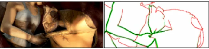
Figure 2. Example of depth discontinuities (in red) and motion boundaries (in green, extracted from the ground-truth flow). No-tice how flow discontinuities differ from depth discontinuities. In addition, the presence of non-rigid objects causes most motion boundaries to form non-closed contours.

to estimate optical flow in textureless images. They propose a bottom-up approach to track and group hypothetical mo-tion edge fragments. However, their approach heavily de-pends on the preliminary detection of edge fragments, and is not applicable to realistic videos with textures. Further-more, none of these approaches are based on learning the relation between local features and motion boundaries.

Closely related to estimating motion boundaries is the task of segmenting a video frame into different regions with coherent motion, referred to as layers [11,35]. Recently, several works have considered the joint estimation of mo-tion layers and optical flow [7,29,31]. However, the joint task is challenging, and these methods depend on a com-plex minimization of non-convex energy functions. As a result, the estimation is unreliable for difficult, yet common cases, such as videos with fast motion, large displacements or compression artifacts. More generally, motion layer seg-mentation can be ill-defined, as there exist cases where mo-tion boundaries form non-closed regions, see Figure2. Occlusion detection and boundaries. The related task of occlusion boundary detection has recently received some at-tention [16,30,17]. Occlusion boundaries refer to depth discontinuities. They can correspond to motion boundaries, as they can create differences in flow when the camera or the objects are moving. However, in many cases two re-gions of different depth can have the same flow, see Fig-ure2 where many of the depth discontinuities actually do not correspond to motion boundaries. Most approaches for occlusion boundary detection [30,16,27] rely on an over-segmentation of the image, using for instance [1], followed by a merging procedure. Like our approach, they all use temporal information as a cue, e.g. as the difference be-tween consecutive images [30]. Nevertheless, the final re-sult highly depends on the optical flow accuracy, while our method is robust to failures in the optical flow.

Learning methods for edge and occlusion detection. Re-cent work casts the edge and occlusion detection tasks into a learning framework [12,17]. These approaches rely on a random forest classifier applied to features extracted in a local neighborhood. The approach of [17] for occlusion detection takes as input optical flow estimated with four different algorithms and learns pixel-wise random forests.

input patch Image

Optical flow

Structured output

Figure 3. Illustration of the prediction process with our structured decision tree. Given an input patch from the left image (repre-sented here by image and flow channels), we predict a binary boundary mask, i.e., a leaf of the tree. Predicted masks are aver-aged across all trees and all overlapping patches to yield the final soft-response boundary map.

In contrast, our method leverages information at the patch level and is robust to failures in the optical flow by using an estimated flow error. Dollar and Zitnick [12] use structured random forests for edge detection, which is shown to out-perform the state of the art. We build on their approach and show how to extend it to motion boundary detection.

3. Learning motion boundary detection

In this section, we first present the structured random forests approach. We then detail the set of cues used for motion boundary detection.

3.1. Structured Random Forests

We propose to cast the prediction of local motion bound-ary masks as a learning task using structured random forests. Motion boundaries in a local patch often have similar patterns, e.g. straight lines, parallel lines or T-junctions. The structured random forest framework lever-ages this property by predicting boundaries at the patch level. In practice, several trees are learned independently with randomization on the feature set, leading to a forest of decision trees. Each tree takes as input a patch and pre-dicts a structured output, here a boundary patch. Given an input image, the predictions of each tree (Figure3) for each (overlapping) local patch are averaged in order to yield a fi-nal soft boundary response map. Structured random forests have a good performance and are extremely fast to evaluate. We now describe the learning model in more detail. Here, a decision tree ft(x) is a structured classifier that

takes an input N × N patch with K channels, vectorized as x ∈ RKN2_{, and returns a corresponding binary edge map}

y ∈ BN2

. Internally, each tree fthas a binary structure, i.e.,

each node is either a leaf or has two child nodes. During in-ference, a binary split function h(x, θj) ∈ {0, 1} associated

to each node j is evaluated to decide whether the sample x descends the left or right branch of the tree until a leaf

is reached. The output y associated to the leaf at training time is then returned. The whole process is illustrated in Figure3.

The split functions h(x, θ) considered in this work are ef-ficient decision stumps of two forms: (i) a thresholding op-eration on a single component of x. In this case, θ = (k, τ ) and h1(x, θ) = [x(k) < τ ], where [.] denotes the indicator

function; (ii) a comparison between two components of x. Thus, θ = (k1, k2, τ ) and h2(x, θ) = [x(k1) − x(k2) < τ ].

We choose the same training algorithm for learning the random forest model as [12], using the publicly available code1_{. The success of our approach lies in the choice and}

design of the features, which we now detail.

3.2. Spatial and Temporal Cues

We consider here static appearance features and tempo-ral features to predict motion boundaries. We use the in-dex t to denote the frame for which we predict the motion boundaries (t + 1 being the next frame).

Color (13 channels). We use the three RGB channels in addition to 10 gradient maps, computed in the luminance channel from the Lab color space. We compute the norm of the gradient and oriented gradient maps in 4 directions, both at coarse and fine scales, resulting in (1 + 4) × 2 channels. Optical flow (7 channels). We also use the optical flow wt,t+1between frame t and t+1. Let u and v be the

compo-nents of wt,t+1. In addition to u and v channels, we use an

unoriented gradient map computed aspk∇uk2_{+ k∇vk}2_,

and oriented gradient maps (again at 4 orientations) where the gradient orientation is obtained by averaging the orien-tations of ∇u and ∇v, weighted by their magnitudes. Con-trary to the RGB case, we compute these 5 gradient maps at a coarse scale only. We found that adding the fine scale does not improve the results, probably due to the blur in optical flow estimation. To compute the optical flow, we experi-ment with different state-of-the-art algorithms and compare their performance in Section5.

Image warping errors (2 channels). Optical flow esti-mation can often be partially incorrect. For instance, in Figure 4(c), some object motions are missing (spear) and some others are incorrect (feet). To handle these errors, we propose to add channels indicating where the flow estima-tion is likely to be wrong, see Figure 4(d). To this end, we measure how much the color and gradient constancy assumptions [6,32] are violated. We compute the image warping error, which is defined at a pixel p as ED(p) =

kDt(p) − Dt+1(p + wt,t+1(p))k₂, where D is an image

representation dependent on which constraint (color or gra-dient) is considered. For the color case, D corresponds to the Lab color-space, in which Euclidean distance is closer to perceived color distances. For the gradient case, D is a pixel-wise histogram of oriented gradients (8 orientations),

(a) image (b) ground-truth flow

(c) estimated flow (Classic+NL) (d) image warping error

Figure 4. Illustration of the image warping error (d) computed for the image in (a) and the estimated flow in (c). The ground-truth flow is shown in (b). Errors in flow estimation clearly appear in (d), e.g. for the spear, the dragon’s claws or the character’s feet.

individually normalized to unit norm. We set the warping error to 0 for pixels falling outside the image boundaries. Backward flow and error (9 channels). There is no reason to consider that the forward flow may provide better infor-mation for detecting motion boundaries than the backward flow. Consequently, we add the same 7 channels of optical flow and the 2 channels of image warping errors with the backward flow wt,t−1.

Summary. By concatenating all these channels, we ob-tain a feature representation at the patch level that com-bines several cues: appearance, motion and confidence in motion. The feature representation includes 31 channels in total. Since the 32×32 patches are subsampled by a factor 2 when fed to the classifiers, the final dimension for an input vector x is (32/2)2_{× 31 = 7936.}

4. Datasets and evaluation protocol

In this section, we first present existing optical flow datasets used to train and evaluate our approach. We then introduce our YouTube Motion Boundaries (YMB) dataset and explain the evaluation protocol.

4.1. Optical flow datasets

For training and evaluating our approach, we rely on two state-of-the-art optical flow datasets: Middlebury and MPI-Sintel. Both come with dense ground-truth optical flow, which allows to extract ground-truth motion boundaries. The Middlebury dataset [3] is composed of 8 training se-quences of 2 to 8 frames with ground-truth optical flow for a central frame. Although this dataset contains complex mo-tions, they are limited to small displacements. Thus, the average endpoint error of state-of-the-art optical flow meth-ods is low, around 0.2 pixel.

The MPI-Sintel dataset [10] is composed of animated se-quences generated using computer graphics. Ground-truth optical flow is available for each frame. We only use the training set, as ground-truth flows are not available for the

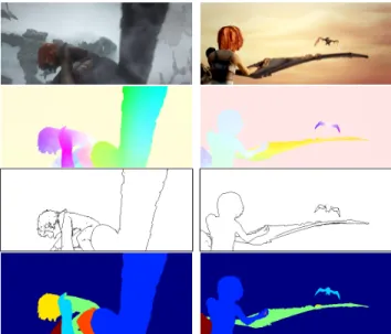
Figure 5. From top to bottom: example images, corresponding ground-truth flow, ground-truth motion boundaries and motion layers used for training.

test set. The training set contains 23 high resolution se-quences of 20 to 50 frames. The presence of fast motion and large occluded areas makes optical flow estimation chal-lenging. This dataset is available in two versions: clean and final. In the final version, realistic effects (e.g. atmospheric fading, motion blur) are included, making the dataset even more challenging for optical flow estimation. We compare results for both versions in the experiments, see Section5. We train our model using all sequences, except when testing on MPI-Sintel. In this case, we alternatively train on half of the sequences and test on the other half.

Ground-truth motion boundaries from flow. For evalu-ation, we need to compute binary motion boundaries from ground-truth optical flow. However, the resulting bound-aries depend on a threshold applied to the norm of the flow gradient. We, thus, propose to generate, for each image, several versions of ground-truth boundaries corresponding to different thresholds. Thresholds are spread regularly on a logarithmic scale. For our experimental evaluation, we have set the lowest threshold to a norm of 0.5 for Middlebury and to 1 for MPI-Sintel. Note that the threshold for Middle-bury is lower than for MPI-Sintel, as motions in this dataset are smaller. Examples for ground-truth motion boundaries (extracted at norm 2) are shown in Figure5. We refer to Section4.3for the evaluation protocol.

4.2. The YMB dataset

Existing optical flow benchmarks have several limita-tions. They are often restricted to synthetic and high qual-ity videos and have limited variabilqual-ity. For instance, MPI-Sintel contains 23 synthetic sequences sharing characters,

Figure 6. Illustration of our YMB dataset. The two left examples comes from YouTube Objects, the three other ones from Sports1M. Top: images. Middle: human annotations of motion boundaries. Bottom: our predictions.

Videos from #videos resolution #annotated px max kwk2 mean kwk2 YouTube Objects [25] 30 225×400 700 (0.7%) 16 5

Sports1M [18] 30 1280×720 3200 (0.3%) 50 8 Table 1. Some statistics of our YMB dataset (averaged across the videos for each part). w denotes the flow, here estimated with LDOF [8].

objects and backgrounds.

Therefore, we propose a new dataset, the YouTube Mo-tion Boundaries dataset (YMB), composed of 60 real-world videos sequences, ranging from low to moderate qual-ity, with a great variability of persons, objects and poses. For each sequence, motion boundaries are manually anno-tated in one frame by three independent annotators. The dataset includes two types of videos: 30 sequences from the YouTube Objects dataset [25], and 30 others from the Sports1M [18] dataset.

YouTube Objects dataset [25] is a collection of video shots representing 10 object categories, such as train, car or dog. For the sake of diversity, we select 3 shots per cate-gory. The annotated frame is the same as the one annotated by Prest et al. [25] for object detection.

Another 30 sequences are sampled from the Sports1M [18] dataset. This dataset comprises 487 classes and is dedicated to action recognition in YouTube videos. We select each video from a different class. The annotated frame is chosen to be challenging for optical flow estimation, see Figure6.

Table1shows some statistics about image sizes and mo-tions. Videos from YouTube Objects have a lower resolu-tion (225×400) than the ones from Sports1M (1280×720). Both datasets contain large motions, some of them of thin parts, e.g. the limbs of the humans. Note that a supplemen-tary challenge of the YMB dataset is due to the high com-pression level of the videos, which causes many block-like

artifacts to appear.

We evaluate the consistency between the annotations. To this end, we compute precision and recall using the proto-col described below (Section 4.3), using one annotator as ground-truth, another one as estimate, and averaging across all pairs of annotators. We obtain a precision and recall over 91%, showing that the annotations are consistent.

4.3. Evaluation protocol

We quantitatively evaluate our motion boundary predic-tions in term of precision-recall. We use the evaluation code of the BSDS [21]2 _{edge detection benchmark. Given}

a binary ground-truth and a soft-response motion bound-ary prediction, we compute the pixel-wise recall and preci-sion curve (Figure10), where each point of the curve cor-responds to a different threshold on the predicted motion boundary strength. For instance, a high threshold will lead to few predicted pixels, i.e., a low recall and high precision. For a lower threshold, the recall will be higher but the pre-cision will drop. To avoid issues related to the over/under-assignment of ground-truth and predicted pixels, a non-maxima suppression step is performed on the predicted mo-tion boundary map, and a bipartite graph problem is solved to perform a 1-to-1 assignment between each detected and ground-truth boundary pixel.

Precision-recall curves are finally averaged for all im-ages and all binary versions of the ground-truth (i.e., anno-tations for the YMB dataset, thresholded maps for the flow benchmarks) to compute mean Average-Precision (mAP). In other words, for optical flow benchmarks, the stronger is a motion boundary, the higher is its impact on the evaluation score.

5. Experimental results

In this section, we first give details on how we train the structured random forest. We then evaluate different aspects of the method, in particular the impact of optical flow algo-rithms and different cues. Furthermore, we compare our approach to various baselines.

5.1. Training the forest

Training random forests typically requires a large num-ber of examples in order to learn a model that generalizes well. MPI-Sintel constitutes an excellent choice for training our model, as the dataset is large and comes with reliable ground-truth flow.

Generating motion layers. When training each node, Dol-lar and Zitnick [12] map the output structured labels (i.e., edge map of a patch) into a set of discrete labels that group similar structured labels. However, computing similarities between edge maps of patches is not well defined. Conse-quently, they propose to approximate it by computing a dis-tance based on the ground-truth segmentation of the image. In the same spirit, training our motion boundary detector will require a segmentation, i.e., motion layers, in addition to the ground-truth motion boundary patches. We now de-scribe the method we use to compute motion layers from the ground-truth optical flow.

We employ a hierarchical clustering approach on flow pixels, where each pixel is connected to its 4 neighbors with a connection weight set to the magnitude of the flow difference between them. From this initial graph, we then grow regions using average linkage by iteratively merging regions with the lowest connection weight. For each im-age, we generate 3 segmentations, with different number of target regions and with randomness in the clustering pro-cess. Generating several segmentations helps to deal with the intrinsic ambiguity of motion layers, whose boundaries only partially correspond to motion boundaries, e.g. in the case of deformable objects, see Figure2. Examples of the resulting segmentation are shown in Figure5(bottom). Random forest parameters. The parameters of the struc-tured random forest are the following. The forest has 8 trees, each with a maximum depth of 64 levels. Trees are trained using a pool of 500k patches containing boundaries and 500k without any boundary. To introduce randomiza-tion in the tree structure, each tree is trained from a random subset (25%) of all training patches.

Clean versus final version. The training set of MPI-Sintel comes in two different versions (clean and final). We con-duct an experiment in which we train two separate models, one for each set. Their performance on the different datasets is evaluated in Table2using Classic+NL [28] flow estima-tion. It turns out that, surprisingly, results are consistently better across all datasets when the model is trained on the clean version of MPI-Sintel – even when detecting motion

Training / Test Middlebury MPI-Sintel clean MPI-Sintel final YMB train on clean 91.1 76.3 68.5 72.2 train on final 90.9 74.6 67.6 70.7 Table 2. Comparison of the performance (mAP) of our motion boundary estimation, when training on the clean or the final ver-sion of the MPI-Sintel dataset. The flow is estimated with Clas-sic+NL [28].

Ground-Truth Farneback

TV-L1 Classic+NL

LDOF DeepFlow

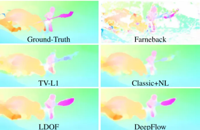
Figure 7. Optical flow estimated with different methods.

boundaries on the final version. This might be explained by the fact that training is affected by noise, which is de factoabsent from the clean set. In contrast, noise is clearly present in the final version, in particular in the form of mo-tion blur that tends to smooth evidence of momo-tion bound-aries. This result is confirmed for all the optical flow al-gorithms evaluated. We, thus, choose the clean version of MPI-Sintel to train our models in the remainder of the ex-periments.

5.2. Impact of the optical flow algorithm

Our approach relies on several temporal cues, see Sec-tion3.2. These cues directly depend on the algorithm used to estimate the optical flow. We compare five different al-gorithms: Farneback [13], TV-L1 [37], Classic+NL [28], LDOF [8] and DeepFlow [36], see Figure7. We can ob-serve that Farneback’s approach results in a noisy estima-tion and is unreliable in untextured regions. The reason is that this approach is local and does not incorporate a global regularization. The four other approaches minimize a global energy using a coarse-to-fine scheme. TV-L1 uses the dual space for minimizing this energy. A fixed point it-erations allows the three remaining approaches to obtain the linear system of equations derived from the energy. They, thus, produce more accurate flow estimations, see Figure7. Classic+NL includes an additional non-local smoothness term that enhances the sharpness of motion boundaries. For instance, the contour of the character is better respected than with the other methods. LDOF and DeepFlow inte-grate a descriptor matching term, allowing to better handle large displacements. This is visible on the spear in

Fig-Middlebury MPI-Sintel clean MPI-Sintel final YMB flow MB ours flow MB ours flow MB ours flow MB ours Farneback 26.6 66.0 18.4 60.0 19.3 52.2 28.4 59.4 TV-L1 78.4 85.7 44.3 73.0 38.1 62.7 45.4 70.1 Classic+NL 90.5 91.1 68.5 76.3 58.0 68.5 59.4 72.2 LDOF 70.2 86.7 50.7 75.2 42.0 65.6 48.9 70.5 DeepFlow 80.6 89.0 56.9 75.8 46.3 67.7 44.7 68.6

Table 3. Comparison of the performance (mAP) of our approach for different input flows. We also compare to a baseline of motion boundaries directly computed from the flow (flow MB).

ure7, whose motion is partially captured. DeepFlow im-proves over LDOF in the matching scheme, making it cur-rently top-performer on MPI-Sintel [10]. Both DeepFlow and LDOF tend to over-smooth the flow: for instance, the motion of the spear spreads in the background.

For each of these flows, we train a separate model and report mean Average-Precision (mAP) for all datasets in Table3. The performance of our approach is rather inde-pendent of the flow algorithm used, with the exception of Farneback’s method which results in a significantly worse performance. Classic+NL gives the best performance on all datasets. This can be explained by the sharpness of the flow boundaries thanks to the non-local regularization.

5.3. Comparison to a state-of-the-art baseline

In Table3, we compare our method to baseline motion boundaries, extracted as the gradient norm of each flow. Note that the performance of our approach largely outper-forms this baseline, for all flow methods and on all datasets. The gap is especially large for the most challenging datasets (e.g. +25% in mAP for LDOF on MPI-Sintel and YMB). Note that results on Middlebury and YMB datasets are ob-tained with the model trained on MPI-Sintel. This demon-strates that our approach for motion boundary estimation performs well on low-resolution YouTube videos despite the fact that it was trained on synthetic high resolution data from MPI-Sintel. In addition, this shows that our method generalizes well to another dataset with different content and does not require specific tuning.

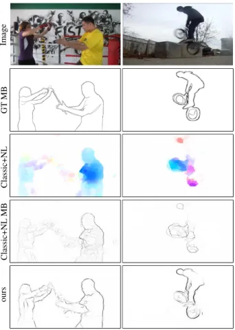
Figure8provides qualitative comparisons between Clas-sic+NL flow boundaries and our predictions for two images from MPI-Sintel [10]. Some object motions, like the char-acter in the left column, are missed in the flow estimation. Likewise, errors due to over-smoothing are visible at the bottom of the right column. They are well recovered by our model, which accurately predicts the motion bound-aries. The robustness of our model to incorrect or over-smooth flow estimates is confirmed by the examples from YMB shown in Figure9. The motion of the arm is badly estimated by the flow (left) and the motion of the wheels (right) spreads in the background. In both cases, our model is able to accurately estimate motion boundaries. This

re-Image GT flo w GT MB Classic+NL Classic+NL MB ours

Figure 8. Example results from the MPI-Sintel dataset with, from top to bottom: image, ground-truth flow, ground-truth motion boundaries, flow estimation using Classic+NL [28], norm of the flow gradient (Classic+NL MB), and the motion boundaries esti-mated by our method (ours).

silience can be explained by the integration of appearance and flow confidence cues (Section3.2) in our model, which certainly helps the classifier to recover from errors in the flow estimation, as shown in the next section.

5.4. Impact of the temporal cues

We conduct an ablative study to determine the impor-tance of the temporal cues used as feature channels by the classifier. Table4shows the improvements resulting from adding one cue at a time. In addition, Figure10shows the precision recall curves for the MPI-Sintel dataset. Perfor-mance is reported for Classic+NL, but all flow estimators

Image GT MB Classic+NL Classic+NL MB ours

Figure 9. Example results from the YMB dataset with, from top to bottom: images, annotated motion boundaries, flow estimation using Classic+NL [28], norm of the flow gradient (Classic+NL MB), and the motion boundaries estimated by our method (ours).

channels used Middlebury MPI-Sintel YMB clean final SED [12] 48.8 32.4 30.1 31.3 RGB only 48.0 41.1 37.5 36.3 +Flow 91.8 72.2 66.3 69.6 +Image warping error 91.2 74.2 66.1 70.5 +Backward flow&error 91.1 76.3 68.5 72.2 Table 4. Importance of temporal cues for predicting motion bound-aries. We also compare to SED [12] that uses the same framework, learned on different data.

result in a similar behavior.

First, we notice that using static cues alone already out-performs the SED edge detector [12], which uses the same RGB cues and learning approach, but a different training set. This indicates that, based on appearances cues alone, one is able to ‘learn’ the location of motion boundaries. Af-ter examining the decision tree, we find that, in this case, the classifier learns that a color difference between two objects is likely to yield a motion boundary.

On Middlebury, using only the first two cues (appearance and flow) suffices to accurately predict motion boundaries.

0.0 0.2 0.4 0.6 0.8 1.0 recall 0.0 0.2 0.4 0.6 0.8 1.0 precision

Result AP curves on MPI-Sintel (clean version)

SED edges Ours, RGB only Ours, +Flow

Ours, +Image warping error Ours, +Backward flow & error

Figure 10. Precision-recall curves when studying the importance of temporal cues on MPI-Sintel dataset, clean version.

0.00 0.01 0.02 0.03 0.04 0.05 0.06

color gradient flow flow gradient BW flow BW flow gradient color er ror grad er ror BW color er ror BW grad erro r

Figure 11. Frequency of each feature channel in the decision stumps of the random forest learned on MPI-Sintel clean. ‘BW’ refers to backward, ‘color error’ (resp. ‘grad error’) denotes the color-based (resp. gradient-based) image warping error. All chan-nels are about equally important.

The initial flow estimate is already very close to the ground-truth for this relatively easy dataset. On the more challeng-ing datasets (MPI-Sintel and YMB), addchalleng-ing the flow con-fidence cue (i.e., image warping errors) allows to further gain up to 2% in mean Average-Precision. As shown in Figure4, the error maps indeed accurately indicate errors in the flow estimation. Finally, backward flow cues lead to an additional gain of 2%. We also conduct an analysis of the frequency of usage of each channel in the decision stumps of our learned forest. Figure11plots the resulting histogram, which confirms that, overall, all channels have approximately the same importance.

6. Conclusion

In this work, we have demonstrated that a learning-based approach using structured random forests is successful for detecting motion boundaries. Thanks to the integration of diverse appearance and temporal cues, our approach is re-silient to errors in flow estimation. Our approach outputs ac-curate motion boundaries and largely outperforms baseline flow-based motion boundaries, in particular on challenging video sequences with large displacements, motion blur and compression artifacts. Future work will include improving optical flow based on these motion boundaries.

Acknowledgments

This work was supported by the European integrated project AXES, the MSR-Inria joint centre, the LabEx Persyval-Lab (ANR-11-LABX-0025), the Moore-Sloan Data Science Environment at NYU, and the ERC advanced grant ALLEGRO.

References

[1] P. Arbelaez, M. Maire, C. Fowlkes, and J. Malik. Contour detection and hierarchical image segmentation. IEEE Trans. PAMI, 2011.2

[2] S. Baker and I. Matthews. Lucas-Kanade 20 years on: A unifying framework. IJCV, 2004.1

[3] S. Baker, D. Scharstein, J. P. Lewis, S. Roth, M. J. Black, and R. Szeliski. A database and evaluation methodology for optical flow. IJCV, 2011.4

[4] S. T. Birchfield. Depth and motion discontinuities. PhD the-sis, Stanford University, 1999.1

[5] M. J. Black and D. J. Fleet. Probabilistic detection and track-ing of motion boundaries. IJCV, 2000.1,2

[6] T. Brox, A. Bruhn, N. Papenberg, and J. Weickert. High ac-curacy optical flow estimation based on a theory for warping. In ECCV, 2004.1,3

[7] T. Brox, A. Bruhn, and J. Weickert. Variational motion seg-mentation with level sets. In ECCV. 2006.2

[8] T. Brox and J. Malik. Large displacement optical flow: de-scriptor matching in variational motion estimation. IEEE Trans. PAMI, 2011.5,6

[9] A. Bruhn, J. Weickert, C. Feddern, T. Kohlberger, and C. Schn¨orr. Variational optical flow computation in real time. IEEE Trans. on Image Processing, 2005.1

[10] D. J. Butler, J. Wulff, G. B. Stanley, and M. J. Black. A naturalistic open source movie for optical flow evaluation. In ECCV, 2012.2,4,7

[11] T. Darrell and A. Pentland. Cooperative robust estimation using layers of support. IEEE Trans. PAMI, 1995.2

[12] P. Doll´ar and C. L. Zitnick. Structured forests for fast edge detection. In ICCV, 2013.2,3,6,8

[13] G. Farneb¨ack. Two-frame motion estimation based on poly-nomial expansion. In Scandinavian conference on Image analysis, 2003.6

[14] D. J. Fleet, M. J. Black, Y. Yacoob, and A. D. Jepson. Design and use of linear models for image motion analysis. IJCV, 2000.2

[15] L. Gorelick, M. Blank, E. Shechtman, M. Irani, and R. Basri. Actions as space-time shapes. IEEE Trans. PAMI, 2007.1

[16] D. Hoiem, A. Efros, and M. Hebert. Recovering occlusion boundaries from an image. IJCV, 2011.2

[17] A. Humayun, O. Mac Aodha, and G. J. Brostow. Learning to Find Occlusion Regions. In CVPR, 2011.2

[18] A. Karpathy, G. Toderici, S. Shetty, T. Leung, R. Sukthankar, and L. Fei-Fei. Large-scale video classification with convo-lutional neural networks. In CVPR, 2014.5

[19] I. Laptev and P. P´erez. Retrieving actions in movies. In ICCV, 2007.1

[20] C. Liu, W. T. Freeman, and E. H. Adelson. Analysis of con-tour motions. In Advances in Neural Information Processing Systems, 2006.2

[21] D. Martin, C. Fowlkes, D. Tal, and J. Malik. A database of human segmented natural images and its application to evaluating segmentation algorithms and measuring ecologi-cal statistics. In ICCV, 2001.5

[22] M. Middendorf and H. Nagel. Estimation and interpretation of discontinuities in optical flow fields. In ICCV, 2001.1

[23] P. Nillius, J. Sullivan, and S. Carlsson. Multi-target track-ing - linktrack-ing identities ustrack-ing Bayesian network inference. In CVPR, 2006.1

[24] A. Papazoglou and V. Ferrari. Fast object segmentation in unconstrained video. In ICCV, 2013.1,2

[25] A. Prest, C. Leistner, J. Civera, C. Schmid, and V. Fer-rari. Learning object class detectors from weakly annotated video. In CVPR, 2012.5

[26] A. Spoerri. The Early Detection of Motion Boundaries. PhD thesis. Massachusetts Institute of Technology, Department of Brain and Cognitive Sciences, 1991.1,2

[27] A. Stein and M. Hebert. Occlusion boundaries from motion: Low-level detection and mid-level reasoning. IJCV, 2009.2

[28] D. Sun, S. Roth, and M. Black. A quantitative analysis of current practices in optical flow estimation and the principles behind them. IJCV, 2014.1,2,6,7,8

[29] D. Sun, J. Wulff, E. B. Sudderth, H. Pfister, and M. J. Black. A fully-connected layered model of foreground and back-ground flow. In CVPR, 2013.2

[30] P. Sundberg, T. Brox, M. Maire, P. Arbelaez, and J. Malik. Occlusion boundary detection and figure/ground assignment from optical flow. In CVPR, 2011.2

[31] M. Unger, M. Werlberger, T. Pock, and H. Bischof. Joint motion estimation and segmentation of complex scenes with label costs and occlusion modeling. In CVPR, 2012.2

[32] C. Vogel, S. Roth, and K. Schindler. An evaluation of data costs for optical flow. In GCPR, 2013.3

[33] S. Volz, A. Bruhn, L. Valgaerts, and H. Zimmer. Modeling temporal coherence for optical flow. In ICCV, 2011.1

[34] H. Wang, A. Kl¨aser, C. Schmid, and C.-L. Liu. Dense tra-jectories and motion boundary descriptors for action recog-nition. IJCV, 2013.1,2

[35] J. Wang and E. Adelson. Representing moving images with layers. IEEE Trans. Image Processing, 1994.2

[36] P. Weinzaepfel, J. Revaud, Z. Harchaoui, and C. Schmid. Deepflow: Large displacement optical flow with deep match-ing. In ICCV, 2013.6

[37] C. Zach, T. Pock, and H. Bischof. A duality based approach for realtime tv-l 1 optical flow. Pattern Recognition, 2007.6