HAL Id: hal-02499206
https://hal.inria.fr/hal-02499206v2
Submitted on 6 Jan 2021
HAL is a multi-disciplinary open access archive for the deposit and dissemination of sci-entific research documents, whether they are pub-lished or not. The documents may come from teaching and research institutions in France or abroad, or from public or private research centers.
L’archive ouverte pluridisciplinaire HAL, est destinée au dépôt et à la diffusion de documents scientifiques de niveau recherche, publiés ou non, émanant des établissements d’enseignement et de recherche français ou étrangers, des laboratoires publics ou privés.
to Basic Feasible Functions
Emmanuel Hainry, Romain Péchoux
To cite this version:
Emmanuel Hainry, Romain Péchoux. Theory of Higher Order Interpretations and Application to Basic Feasible Functions. Logical Methods in Computer Science, Logical Methods in Computer Science Association, 2020, 16 (4), pp.25. �10.23638/LMCS-16(4:14)2020�. �hal-02499206v2�
THEORY OF HIGHER ORDER INTERPRETATIONS AND APPLICATION TO BASIC FEASIBLE FUNCTIONS
EMMANUEL HAINRY AND ROMAIN P ´ECHOUX
Universit´e de Lorraine, CNRS, Inria, LORIA, F-54000 Nancy, France e-mail address: {emmanuel.hainry,romain.pechoux}@loria.fr
Abstract. Interpretation methods and their restrictions to polynomials have been deeply used to control the termination and complexity of first-order term rewrite systems. This paper extends interpretation methods to a pure higher order functional language. We develop a theory of higher order functions that is well-suited for the complexity analysis of this programming language. The interpretation domain is a complete lattice and, consequently, we express program interpretation in terms of a least fixpoint. As an application, by bounding interpretations by higher order polynomials, we characterize Basic Feasible Functions at any order.
1. Introduction
1.1. Higher order interpretations. This paper introduces a theory of higher order in-terpretations for studying higher order complexity classes. These inin-terpretations are an extension of usual (polynomial) interpretation methods introduced in [MN70, Lan79] and used to show the termination of (first order) term rewrite systems [CMPU05, CL92] or to study their complexity [BMM11].
This theory is a novel and uniform extension to higher order functional programs: the definition works at any order on a simple programming language, where interpretations can be elegantly expressed in terms of a least fixpoint, and no extra constraints are required.
The language has only one semantics restriction: its reduction strategy is enforced to be leftmost outermost as interpretations are non decreasing functions. Similarly to first order interpretations, higher order interpretations ensure that each reduction step corresponds to a strict decrease. Consequently, some of the system properties could be lost if a reduction occurs under a context.
Key words and phrases: Implicit computational complexity, basic feasible functionals.
This work has been partially supported by ANR Project ELICA ANR-14-CE25-0005 and Inria associate team TC(Pro)3.
LOGICAL METHODS
l
IN COMPUTER SCIENCE DOI:10.23638/LMCS-16(4:14)2020© E. Hainry and R. Péchoux
CC
1.2. Application to higher order polynomial time. As Church-Turing’s thesis does not hold at higher order, distinct and mostly pairwise incomparable complexity classes are candidates as a natural equivalent of the notion of polynomial time computation for higher order.
The class of polynomially computable real functions by Ko [Ko91] and the class of Basic Feasible Functional at order 𝑖 (bff𝑖) by Irwin, Kapron and Royer [IKR02] belong to the
most popular definitions for such classes. In [Ko91] polynomially computable real functions are defined in terms of first order functions over real numbers. They consist in order 2 functions over natural numbers and an extension at any order is proposed by Kawamura and Cook in [KC10]. The main distinctions between these two models are the following: ∙ the book [Ko91] deals with representation of real numbers as input while the paper [IKR02]
deals with general functions as input,
∙ the book [Ko91] deals with the number of steps needed to produce an output at a given precision while the paper [IKR02] deals with the number of reduction steps needed to evaluate the program.
Moreover, it was shown in [IKR02] and [F´er14] that the classes bff𝑖 cannot capture
some functions that could be naturally considered to be polynomial time computable because they do not take into account the size of their higher order arguments. However they have been demonstrated to be robust, they characterize exactly the well-known class fptime of polynomial time computable functions as well as the well-known class of Basic Feasible Functions bff, that corresponds to order 2 polynomial time computations, and have already been characterized in various ways, e.g. [CK89].
The current paper provides a characterization of the bff𝑖 classes as they deal with
discrete data as input and they are consequently more suited to be studied with respect to usual functional languages. This result was expected to hold as it is known for a long time that (first order) polynomial interpretations characterize fptime and as it is shown in [FHHP15] that (first order) polynomial interpretations on stream programs characterize bff.
1.3. Related works. The present paper is an extended version of the results in [HP17]: more proofs and examples have been provided. An erratum has been provided: the interpretation of the case construct has been slightly modified so that we can consider non decreasing functions (and not only strictly increasing functions).
There are two lines of work that are related to our approach. In [VdP93], Van de Pol introduced higher order interpretation for showing the termination of higher order term rewrite systems. In [BL12, BL16], Baillot and Dal Lago introduce higher order interpretations for complexity analysis of term rewrite systems. While the first work only deals with termination properties, the second work is restricted to a family of higher order term rewrite systems called simply typed term rewrite systems. Our work can be viewed as an extension of [BL16] to functional programs and polynomial complexity at any order.
1.4. Outline. In Section 2, the syntax and semantics of the functional language are intro-duced. The new notion of higher order interpretation and its properties are described in Section 3. Next, in Section 4, we briefly recall the bff𝑖 classes and their main
characteriza-tions, including a characterization based on the BTLP programming language of [IKR02]. Section 5 is devoted to the characterization of these classes using higher order polynomials.
The soundness relies on interpretation properties: the reduction length is bounded by the interpretation of the initial term. The completeness is demonstrated by simulating a BTLP procedure: compiling procedures to terms after applying some program transformations. In Section 6, we briefly discuss the open issues and future works related to higher order interpretations.
2. Functional language
2.1. Syntax. The considered programming language consists in an unpure lambda calculus with constructors, primitive operators, a 𝚌𝚊𝚜𝚎 construct for pattern matching and a 𝚕𝚎𝚝𝚁𝚎𝚌 instruction for function definitions that can be recursive. It is as an extension of PCF [Mit96] to inductive data types and it enjoys the same properties (confluence and completeness with respect to partial recursive functions for example).
The set of terms of the language is generated by the following grammar:
𝙼, 𝙽 ∶∶= 𝚡| 𝚌 | 𝚘𝚙 | 𝚌𝚊𝚜𝚎 𝙼 𝚘𝚏 𝚌1(⃖⃖⃖⃗𝚡1) → 𝙼1, ..., 𝚌𝑛(⃖⃖⃖⃗𝚡𝑛) → 𝙼𝑛 | 𝙼 𝙽 | 𝜆𝚡.𝙼 | 𝚕𝚎𝚝𝚁𝚎𝚌 𝚏 = 𝙼,
where 𝚌, 𝚌1,⋯ , 𝚌𝑛 are constructor symbols of fixed arity and 𝚘𝚙 is an operator of fixed
arity. Given a constructor or operator symbol 𝑏, we write 𝑎𝑟(𝑏) = 𝑛 whenever 𝑏 is of arity 𝑛. 𝚡, 𝚏 are variables in and ⃖⃖⃗𝚡𝑖 is a sequence of 𝑎𝑟(𝚌𝑖) variables.
The free variables 𝐹 𝑉 (𝙼) of a term 𝙼 are defined as usual. Bounded variables are assumed to have distinct names in order to avoid name clashes. A closed term is a term 𝙼 with no free variables, 𝐹 𝑉 (𝙼) = ∅.
A substitution {𝙽1∕𝚡1,⋯ , 𝙽𝑛∕𝚡𝑛} is a partial function mapping variables 𝚡1,⋯ , 𝚡𝑛 to terms 𝙽1,⋯ , 𝙽𝑛. The result of applying the substitution {𝙽1∕𝚡1,⋯ , 𝙽𝑛∕𝚡𝑛} to a term 𝙼 is noted
𝙼{𝙽1∕𝚡1,⋯ , 𝙽𝑛∕𝚡𝑛} or 𝙼{⃖⃗𝙽∕⃖⃗𝚡} when the substituting terms are clear from the context.
2.2. Semantics. Each primitive operator 𝚘𝚙 has a corresponding semanticsJ𝚘𝚙K fixed by the language implementation. J𝚘𝚙K is a total function from 𝑎𝑟(𝚘𝚙) to
.1 We define the following relations between two terms of the language: ∙ 𝛽-reduction: 𝜆𝚡.𝙼 𝙽 →𝛽 𝙼{𝙽∕𝚡},
∙ pattern matching: case 𝚌𝑗(⃖⃖⃖⃗𝙽𝑗) of … 𝚌𝑗(⃖⃖⃖⃗𝚡𝑗) → 𝙼𝑗… →𝚌𝚊𝚜𝚎 𝙼𝑗{⃖⃖⃖⃗𝙽𝑗∕⃖⃖⃖⃗𝚡𝑗},
∙ operator evaluation: 𝚘𝚙 𝙼1… 𝙼𝑛→𝚘𝚙J𝚘𝚙K(𝙼1,… , 𝙼𝑛),
∙ fixpoint evaluation: 𝚕𝚎𝚝𝚁𝚎𝚌 𝚏 = 𝙼 →𝚕𝚎𝚝𝚁𝚎𝚌𝙼{𝚕𝚎𝚝𝚁𝚎𝚌 𝚏 = 𝙼∕𝚏}.
Let →𝛼 be defined as ∪𝑟∈{𝛽,𝚌𝚊𝚜𝚎,𝚕𝚎𝚝𝚁𝚎𝚌,𝚘𝚙}→𝑟. Let ⇒𝑘 be the leftmost outermost
(normal-order) evaluation strategy defined with respect to →𝛼 in Figure 1. The index 𝑘 accounts for
the number of →𝛼 steps fired during a reduction. Let ⇒ be a shorthand notation for ⇒1. Let |𝙼 ⇒𝑘 𝙽| be the number of reductions distinct from →
𝚘𝚙 in a given a derivation 𝙼 ⇒𝑘 𝙽. |𝙼 ⇒𝑘 𝙽| ≤ 𝑘 always holds. J𝙼K is a notation for the term computed by 𝙼 (if it exists), i.e. ∃𝑘, 𝙼 ⇒𝑘
J𝙼K and ∄𝙽, J𝙼K ⇒ 𝙽.
A (first order) value 𝚟 is defined inductively by either 𝚟 = 𝚌, if 𝑎𝑟(𝚌) = 0, or 𝚟 = 𝚌 ⃖⃗𝚟, for
𝑎𝑟(𝚌) > 0 values ⃖⃗𝚟, otherwise.
1Operators are total functions over terms and are not only defined on “values”, i.e. terms of the shape
𝜆𝚡.𝙼, so that we never need to reduce the operands in rule →𝚘𝚙. This will allow us to consider non decreasing operator interpretations in Definition 3.5 instead of strictly increasing operator interpretation.
𝙼 ⇒𝑘 𝙽 case𝙼 of … ⇒𝑘 case 𝙽 of … 𝙼 ⇒𝑘 𝙼′ 𝙼 𝙽 ⇒𝑘 𝙼′ 𝙽 𝙼 →𝛼 𝙽 𝙼 ⇒1𝙽 𝙼 ⇒𝑘 𝙼′ 𝙼′ ⇒𝑘′ 𝙽 𝙼 ⇒𝑘+𝑘′ 𝙽
Figure 1: Evaluation strategy
Γ(𝚡) = 𝚃 Γ; Δ ⊢ 𝚡 ∶∶ 𝚃 (Var) Δ(𝚌) = 𝚃 Γ; Δ ⊢ 𝚌 ∶∶ 𝚃 (Cons) Δ(𝚘𝚙) = 𝚃 Γ; Δ ⊢ 𝚘𝚙 ∶∶ 𝚃 (Op) Γ; Δ ⊢ 𝙼 ∶∶ 𝚃1⟶ 𝚃2 Γ; Δ ⊢ 𝙽 ∶∶ 𝚃1 Γ; Δ ⊢ 𝙼 𝙽 ∶∶ 𝚃2 (App) Γ, 𝚡 ∶∶ 𝚃1; Δ ⊢ 𝙼 ∶∶ 𝚃2 Γ; Δ ⊢ 𝜆𝚡.𝙼 ∶∶ 𝚃1 → 𝚃2 (Abs) Γ, 𝚏 ∶∶ 𝚃; Δ ⊢ 𝙼 ∶∶ 𝚃 Γ; Δ ⊢ 𝚕𝚎𝚝𝚁𝚎𝚌 𝚏 = 𝙼 ∶∶ 𝚃 (Let) Γ; Δ ⊢ 𝙼 ∶∶ b Γ; Δ ⊢ 𝚌𝑖∶∶ ⃖⃖⃗b𝑖⟶ b Γ, ⃖⃖⃗𝚡𝑖∶∶ ⃖⃖⃗b𝑖; Δ ⊢ 𝙼𝑖∶∶ 𝚃 (1≤ 𝑖 ≤ 𝑚) Γ; Δ ⊢ 𝚌𝚊𝚜𝚎 𝙼 𝚘𝚏 𝚌1(⃖⃖⃖⃗𝚡1) → 𝙼1, ..., 𝚌𝑛(⃖⃖⃖⃗𝚡𝑛) → 𝙼𝑛 ∶∶ 𝚃 (Case)
Figure 2: Type system
2.3. Type system. Let B be a set of basic inductive types b described by their constructor symbol setsb. The set of simple types is defined by:
𝚃 ∶∶= b | 𝚃 ⟶ 𝚃, with b ∈ B. As usual ⟶ associates to the right.
Example 2.1. The type of unary numbers 𝙽𝚊𝚝 can be described by𝙽𝚊𝚝 = {0, +𝟷}, 0 being a constructor symbol of 0-arity and +𝟷 being a constructor symbol of 1-arity.
For any type 𝑇 , [𝑇 ] is the base type for lists of elements of type 𝚃 and has constructor symbol set[𝚃] = {𝚗𝚒𝚕, 𝚌}, 𝚗𝚒𝚕 being a constructor symbol of 0-arity and 𝚌 being a constructor symbol of 2-arity.
The type system is described in Figure 2 and proves judgments of the shape Γ; Δ ⊢ 𝙼 ∶∶ 𝚃 meaning that the term 𝙼 has type 𝚃 under the variable and constructor symbol contexts Γ and Δ respectively ; a variable (a constructor, respectively) context being a partial function that assigns types to variables (constructors and operators, respectively).
As usual, the input type and output type of constructors and operators of arity 𝑛 will be restricted to basic types. Consequently, their types are of the shape b1⟶ … ⟶ b𝑛⟶ b.
A well-typed term will consist in a term 𝙼 such that ∅; Δ ⊢ 𝙼 ∶∶ 𝚃. Consequently, it is mandatory for a term to be closed in order to be well-typed.
In what follows, we will consider only well-typed terms. The type system assigns types to all the syntactic constructions of the language and ensures that a program does not go wrong. Notice that the typing discipline does not prevent a program from diverging. Definition 2.2 (Order). The order of a type 𝚃, noted 𝚘𝚛𝚍(𝚃), is defined inductively by:
𝚘𝚛𝚍(b) = 0, if b ∈ B,
Given a term 𝙼 of type 𝚃, i.e. ∅; Δ ⊢ 𝙼 ∶∶ 𝚃, the order of 𝙼 with respect to 𝚃 is 𝚘𝚛𝚍(𝚃). Example 2.3. Consider the following term 𝙼 that maps a function to a list given as inputs:
𝚕𝚎𝚝𝚁𝚎𝚌 𝚏 = 𝜆g.𝜆𝚡.𝚌𝚊𝚜𝚎 𝚡 𝚘𝚏 𝚌(𝚢, 𝚣) → 𝚌 (g 𝚢) (𝚏 g 𝚣), 𝚗𝚒𝚕 → 𝚗𝚒𝚕.
Let [𝙽𝚊𝚝] is the base type for lists of natural numbers of constructor symbol set [𝙽𝚊𝚝] = {𝚗𝚒𝚕, 𝚌}. The term 𝙼 can be typed by ∅; Δ ⊢ 𝙼 ∶∶ (𝙽𝚊𝚝 ⟶ 𝙽𝚊𝚝) ⟶ [𝙽𝚊𝚝] ⟶ [𝙽𝚊𝚝], as illustrated by the following typing derivation:
⋯ ⋯ ⋯ Γ′; Δ ⊢ (g 𝚢) ∶∶ 𝙽𝚊𝚝 (App) Γ′; Δ ⊢ 𝚌 (g 𝚢) ∶∶ [𝙽𝚊𝚝] ⟶ [𝙽𝚊𝚝] (App) ⋯ Γ′; Δ ⊢ (𝚏 g 𝚣) ∶∶ [𝙽𝚊𝚝] (App) ⋯ Γ, 𝚢 ∶∶ 𝙽𝚊𝚝, 𝚣 ∶∶ [𝙽𝚊𝚝]; Δ ⊢ 𝚌 (g 𝚢) (𝚏 g 𝚣) ∶∶ [𝙽𝚊𝚝] (App) Γ, 𝚡 ∶∶ [𝙽𝚊𝚝]; Δ ⊢ 𝚌𝚊𝚜𝚎 𝚡 𝚘𝚏 𝚌(𝚢, 𝚣) → 𝚌 (g 𝚢) (𝚏 g 𝚣), 𝚗𝚒𝚕 → 𝚗𝚒𝚕 ∶∶ [𝙽𝚊𝚝] (Case) Γ; Δ ⊢ 𝜆𝚡.𝚌𝚊𝚜𝚎 𝚡 𝚘𝚏 𝚌(𝚢, 𝚣) → 𝚌 (g 𝚢) (𝚏 g 𝚣), 𝚗𝚒𝚕 → 𝚗𝚒𝚕 ∶∶ [𝙽𝚊𝚝] ⟶ [𝙽𝚊𝚝] (Abs) 𝚏 ∶∶ 𝚃; Δ ⊢ 𝜆g.𝜆𝚡.𝚌𝚊𝚜𝚎 𝚡 𝚘𝚏 𝚌(𝚢, 𝚣) → 𝚌 (g 𝚢) (𝚏 g 𝚣), 𝚗𝚒𝚕 → 𝚗𝚒𝚕 ∶∶ 𝚃 (Abs) ∅; Δ ⊢ 𝙼 ∶∶ (𝙽𝚊𝚝 ⟶ 𝙽𝚊𝚝) ⟶ [𝙽𝚊𝚝] ⟶ [𝙽𝚊𝚝] (Let)
where 𝚃 is a shorthand notation for (𝙽𝚊𝚝 ⟶ 𝙽𝚊𝚝) ⟶ [𝙽𝚊𝚝] ⟶ [𝙽𝚊𝚝], where the derivation of the base case 𝚗𝚒𝚕 has been omitted for readability and where the contexts Δ, Γ, Γ′ are such that Δ(𝚌) = 𝙽𝚊𝚝 ⟶ [𝙽𝚊𝚝] ⟶ [𝙽𝚊𝚝], Δ(𝚗𝚒𝚕) = [𝙽𝚊𝚝] and Γ = 𝚏 ∶∶ 𝚃, g ∶∶ 𝙽𝚊𝚝 ⟶ 𝙽𝚊𝚝 and Γ′ = Γ, 𝚢 ∶∶ 𝙽𝚊𝚝, 𝚣 ∶∶ [𝙽𝚊𝚝]. Consequently, the order of 𝙼 (with respect to 𝚃) is equal to 2, as 𝚘𝚛𝚍(𝚃) = 2.
3. Interpretations
3.1. Interpretations of types. We briefly recall some basic definitions that are very close from the notions used in denotational semantics (See [Win93]) since, as we shall see later, interpretations can be defined in terms of fixpoints. Let (ℕ,≤, ⊔, ⊓) be the set of natural numbers equipped with the usual ordering≤, a max operator ⊔ and min operator ⊓ and let ℕ be ℕ∪ {⊤}, where ⊤ is the greatest element satisfying ∀𝑛 ∈ ℕ, 𝑛≤ ⊤, 𝑛 ⊔ ⊤ = ⊤ ⊔ 𝑛 = ⊤ and 𝑛 ⊓ ⊤ = ⊤ ⊓ 𝑛 = 𝑛.
The interpretation of a type is defined inductively by:
⦇b⦈ = ℕ, if b is a basic type,
⦇𝚃 ⟶ 𝚃′⦈ = ⦇𝚃⦈ ⟶↑ ⦇𝚃′⦈, otherwise,
where ⦇𝚃⦈ ⟶↑⦇𝚃′⦈ denotes the set of total non decreasing functions from ⦇𝚃⦈ to ⦇𝚃′⦈. A function 𝐹 from the set 𝐴 to the set 𝐵 being non decreasing if for each 𝑋, 𝑌 ∈ 𝐴, 𝑋 ≤𝐴𝑌
implies 𝐹 (𝑋)≤𝐵 𝐹(𝑌 ), where≤𝐴 is the usual pointwise ordering induced by ≤ and defined
by:
𝑛≤ℕ 𝑚iff 𝑛≤ 𝑚,
Example 3.1. The type 𝚃 = (𝙽𝚊𝚝 ⟶ 𝙽𝚊𝚝) ⟶ [𝙽𝚊𝚝] ⟶ [𝙽𝚊𝚝] of the term 𝚕𝚎𝚝𝚁𝚎𝚌 𝚏 = 𝙼 in Example 2.3 is interpreted by:
⦇𝚃⦈ = (ℕ ⟶↑ℕ) ⟶↑ (ℕ ⟶↑ℕ).
In what follows, given a sequence ⃖⃖⃗𝐹 of 𝑚 terms in the interpretation domain and a sequence ⃖⃗𝚃 of 𝑘 types, the notation ⃖⃖⃗𝐹 ∈ ⃖⃖⃖⃖⃖⃗⦇𝚃⦈ means that both 𝑘 = 𝑚 and ∀𝑖 ∈ [1, 𝑚], 𝐹𝑖∈ ⦇𝚃𝑖⦈.
3.2. Interpretations of terms. Each closed term of type 𝚃 will be interpreted by a function in⦇𝚃⦈. The application is denoted as usual whereas we use the notation Λ for abstraction on this function space in order to avoid confusion between terms of our calculus and objects of the interpretation domain. Variables of the interpretation domain will be denoted using upper case letters. When needed, Church typing discipline will be used in order to highlight the type of the bound variable in a lambda abstraction.
An important distinction between the terms of the language and the objects of the interpretation domain lies in the fact that beta-reduction is considered as an equivalence relation on (closed terms of) the interpretation domain, i.e. (Λ𝑋.𝐹 ) 𝐺 = 𝐹 {𝐺∕𝑋} underlying that (Λ𝑋.𝐹 ) 𝐺 and 𝐹 {𝐺∕𝑋} are distinct notations that represent the same higher order function. The same property holds for 𝜂-reduction, i.e. Λ𝑋.(𝐹 𝑋) and 𝐹 denote the same function.
In order to obtain complete lattices, each type ⦇𝚃⦈ has to be completed by a lower bound ⊥⦇𝚃⦈ and an upper bound ⊤⦇𝚃⦈ as follows:
⊥ℕ = 0,
⊤ℕ = ⊤,
⊥⦇𝚃⟶𝚃′⦈ = Λ𝑋⦇𝚃⦈.⊥⦇𝚃′⦈,
⊤⦇𝚃⟶𝚃′⦈ = Λ𝑋⦇𝚃⦈.⊤⦇𝚃′⦈.
Lemma 3.2. For each 𝚃 and for each 𝐹 ∈ ⦇𝚃⦈, ⊥⦇𝚃⦈ ≤⦇𝚃⦈ 𝐹 ≤⦇𝚃⦈ ⊤⦇𝚃⦈. Proof. By induction on types.
Notice that for each type 𝚃 it also holds that ⊤⦇𝚃⦈ ≤⦇𝚃⦈ ⊤⦇𝚃⦈, by an easy induction. In the same spirit, max and min operators ⊔ (and ⊓) over ℕ can be extended to higher order functions 𝐹 , 𝐺 of any arbitrary type ⦇𝚃⦈ ⟶↑ ⦇𝚃′⦈ by:
⊔⦇𝚃⦈⟶↑⦇𝚃′⦈(𝐹 , 𝐺) = Λ𝑋⦇𝚃⦈. ⊔⦇𝚃′⦈(𝐹 (𝑋), 𝐺(𝑋)),
⊓⦇𝚃⦈⟶↑⦇𝚃′⦈(𝐹 , 𝐺) = Λ𝑋⦇𝚃⦈. ⊓⦇𝚃′⦈(𝐹 (𝑋), 𝐺(𝑋)).
In the following, we use the notations ⊥, ⊤, ≤, <, ⊔ and ⊓ instead of ⊥⦇𝚃⦈, ⊤⦇𝚃⦈,≤⦇𝚃⦈, <⦇𝚃⦈,
⊔⦇𝚃⦈ and ⊓⦇𝚃⦈, respectively, when ⦇𝚃⦈ is clear from the typing context. Moreover, given a boolean predicate 𝑃 on functions, we will use the notation ⊔𝑃{𝐹 } as a shorthand notation
for ⊔{𝐹 | 𝑃 }.
Lemma 3.3. For each type 𝚃, (⦇𝚃⦈,≤, ⊔, ⊓, ⊤, ⊥) is a complete lattice.
Proof. Consider a subset 𝑆 of elements in ⦇𝚃⦈ and define ⊔𝑆 = ⊔𝐹∈𝑆𝐹. By definition, we have 𝐹 ≤ ⊔𝑆, for any 𝐹 ∈ 𝑆. Now consider some 𝐺 such that for all 𝐹 ∈ 𝑆, 𝐹 ≤ 𝐺. We have ∀𝐹 ∈ 𝑆, ∀𝑋, 𝐹 (𝑋)≤ 𝐺(𝑋). Consequently, ∀𝑋, 𝑆(𝑋) = ⊔𝐹∈𝑆𝐹(𝑋)≤ 𝐺(𝑋) and 𝑆 is a supremum. The same holds for the infimum.
Now we need to define a unit (or constant) cost function for any interpretation of type 𝚃. For that purpose, let + denote natural number addition extended to ℕ by ∀𝑛, ⊤+𝑛 = 𝑛+⊤ = ⊤. For each type⦇𝚃⦈, we define inductively a dyadic sum function ⊕⦇𝚃⦈ by:
𝑋ℕ⊕ℕ𝑌ℕ= 𝑋 + 𝑌 ,
𝐹 ⊕⦇𝚃⟶𝚃′⦈𝐺= Λ𝑋⦇𝚃⦈.(𝐹 (𝑋) ⊕⦇𝚃′⦈𝐺(𝑋)).
Let us also define the constant function 𝑛⦇𝚃⦈, for each type 𝚃 and each integer 𝑛≥ 1, by:
𝑛ℕ = 𝑛,
𝑛⦇𝚃⟶𝚃′⦈ = Λ𝑋⦇𝚃⦈.𝑛⦇𝚃′⦈.
Once again, we will omit the type when it is unambiguous using the notation 𝑛⊕ to denote the function 𝑛⦇𝚃⦈⊕⦇𝚃⦈ when ⦇𝚃⦈ is clear from the typing context.
For each type⦇𝚃⦈, we can define a strict ordering < by: 𝐹 < 𝐺 whenever 1 ⊕ 𝐹 ≤ 𝐺. Definition 3.4. A variable assignment, denoted 𝜌, is a map associating to each 𝚏 ∈ of type 𝚃 a variable 𝐹 of type ⦇𝚃⦈.
Now we are ready to define the notions of variable assignment and interpretation of a term 𝙼.
Definition 3.5 (Interpretation). Given a variable assignment 𝜌, an interpretation is the extension of 𝜌 to well-typed terms, mapping each term of type 𝚃 to an object in ⦇𝚃⦈ and defined by: ∙ ⦇𝚏⦈𝜌= 𝜌(𝚏), if 𝚏 ∈, ∙ ⦇𝚌⦈𝜌= 1 ⊕ (Λ𝑋1.… .Λ𝑋𝑛. ∑𝑛 𝑖=1𝑋𝑖), if 𝑎𝑟(𝚌) = 𝑛, ∙ ⦇𝙼𝙽⦈𝜌= ⦇𝙼⦈𝜌⦇𝙽⦈𝜌, ∙ ⦇𝜆𝚡.𝙼⦈𝜌= 1 ⊕ (Λ⦇𝚡⦈𝜌.⦇𝙼⦈𝜌), ∙ ⦇case 𝙼 of … 𝚌𝑗(⃖⃖⃖⃗𝚡𝑗) → 𝙼𝑗…⦈𝜌= 1 ⊕ ⊔1≤𝑖≤𝑚⊔⦇𝙼⦈ 𝜌≥⦇𝚌𝑖⦈𝜌⃖⃖⃗𝐹𝑖 {⦇𝙼⦈𝜌⊕⦇𝙼𝑖⦈𝜌{⃖⃖⃖⃗𝐹𝑖∕⃖⃖⃖⃖⃖⃖⃖⃖⃖⃗⦇𝚡𝑖⦈𝜌}}, ∙ ⦇𝚕𝚎𝚝𝚁𝚎𝚌 𝚏 = 𝙼⦈𝜌 = ⊓{𝐹 ∈ ⦇𝚃⦈| 𝐹 ≥ 1 ⊕ ((Λ⦇𝚏⦈𝜌.⦇𝙼⦈𝜌) 𝐹 )}, where ⦇𝚘𝚙⦈𝜌 is a non decreasing total function such that:
∀𝙼1,… , ∀𝙼𝑛, ⦇𝚘𝚙 𝙼1 … 𝙼𝑛⦈𝜌≥ ⦇J𝚘𝚙K(𝙼1,… , 𝙼𝑛)⦈𝜌.
The aim of the interpretation of a term is to give a bound on its computation time as we will shortly see in Corollary 3.11. For that purpose, it requires a strict decrease of the interpretation under ⇒. This is the object of Lemma 3.9. This is the reason why any “construct” of the language involves a 1⊕ in each rule of Definition 3.5. Application that plays the role of a “destructor” does not require this. This is also the reason why the interpretation of a constructor symbol does not depend on its nature.
Remark that the condition on the the interpretation of operators correspond to the notion of sup-interpretation (See [P´ec13] for more details).
3.3. Existence of an interpretation. The interpretation of a term is always defined. Indeed, in Definition 3.5, ⦇𝚕𝚎𝚝𝚁𝚎𝚌 𝚏 = 𝙼⦈𝜌 is defined in terms of the least fixpoint of the function Λ𝑋⦇𝚃⦈.1 ⊕⦇𝚃⦈((Λ⦇𝚏⦈𝜌.⦇𝙼⦈𝜌) 𝑋) and, consequently, we obtain the following result as
a direct consequence of Knaster-Tarski [Tar55, KS01] Fixpoint Theorem: Proposition 3.6. Each term 𝙼 of type 𝚃 has an interpretation.
Proof. By Lemma 3.3, 𝐿 = (⦇𝚃⦈,≤, ⊔, ⊓, ⊤, ⊥) is a complete lattice. The function 𝐹 = Λ𝑋⦇𝚃⦈.1 ⊕⦇𝚃⦈((Λ⦇𝚏⦈𝜌.⦇𝙼⦈𝜌) 𝑋) ∶ 𝐿 → 𝐿 is monotonic. Indeed, both constructor terms and
letRec terms of type ⦇𝚃⦈ are interpreted over a space of monotonic functions ⦇𝚃⦈. Moreover monotonicity is preserved by application, abstraction and the ⊓ and ⊔ operators. Applying Knaster-Tarski, we obtain that 𝐹 admits a least fixpoint, which is exactly ⊓{𝑋 ∈ ⦇𝚃⦈ | 𝑋 ≥
𝐹 𝑋}.
3.4. Properties of interpretations. We now show intermediate lemmata. The following Lemma can be shown by structural induction on terms:
Lemma 3.7. For all 𝙼, 𝙽, 𝚡 such that 𝚡 ∶∶ 𝚃; Δ ⊢ 𝙼 ∶∶ 𝚃′, ∅; Δ ⊢ 𝙽 ∶∶ 𝚃, we have: ⦇𝙼⦈𝜌{⦇𝙽⦈𝜌∕⦇𝚡⦈𝜌} = ⦇𝙼{𝙽∕𝚡}⦈𝜌.
Lemma 3.8. For all 𝙼, 𝙽, 𝚡 such that 𝚡 ∶∶ 𝚃; Δ ⊢ 𝙼 ∶∶ 𝚃′, ∅; Δ ⊢ 𝙽 ∶∶ 𝚃, we have ⦇𝜆𝚡.𝙼 𝙽⦈𝜌 >
⦇𝙼{𝙽∕𝚡}⦈𝜌. Proof. ⦇𝜆𝚡.𝙼 𝙽⦈𝜌= ⦇𝜆𝚡.𝙼⦈𝜌⦇𝙽⦈𝜌 (By Definition 3.5) = (Λ⦇𝚡⦈𝜌.1 ⊕ ⦇𝙼⦈𝜌) ⦇𝙽⦈𝜌 (By Definition 3.5) = 1 ⊕ ⦇𝙼⦈𝜌{⦇𝙽⦈𝜌∕⦇𝚡⦈𝜌} (By definition of =) = 1 ⊕ ⦇𝙼{𝙽∕𝚡}⦈𝜌 (By Lemma 3.7) >⦇𝙼{𝙽∕𝚡}⦈𝜌 (By definition of >)
and so the conclusion.
Lemma 3.9. For all 𝙼, we have: if 𝙼 ⇒ 𝙽 then ⦇𝙼⦈𝜌≥ ⦇𝙽⦈𝜌. Moreover if |𝙼 ⇒ 𝙽| = 1 then ⦇𝙼⦈𝜌 >⦇𝙽⦈𝜌.
Proof. If |𝙼 ⇒ 𝙽| = 0 then 𝙼 = 𝚘𝚙 𝙼1 … 𝙼𝑛 →𝚘𝚙J𝚘𝚙K(𝙼1,… , 𝙼𝑛) = 𝙽, for some operator 𝚘𝚙
and terms 𝙼1,… , 𝙼𝑛 and consequently, by Definition of interpretations we have: ⦇𝚘𝚙 𝙼1 … 𝙼𝑛⦈𝜌≥ ⦇J𝚘𝚙K(𝙼1,… , 𝙼𝑛)⦈𝜌.
If|𝙼 ⇒ 𝙽| = 1 then the reduction is not →𝚘𝚙. By Lemma 3.8, in the case of a 𝛽-reduction and, by induction, by Lemma 3.7 and Definition 3.5 for the other cases. e.g. For a letRec
reduction, we have: if 𝙼 = 𝚕𝚎𝚝𝚁𝚎𝚌 𝚏 = 𝙼′→ 𝚕𝚎𝚝𝚁𝚎𝚌𝙼′{𝙼∕𝚏} = 𝙽 then: ⦇𝙼⦈𝜌= ⊓{𝐹 ∈ ⦇𝚃⦈| 𝐹 ≥ 1 ⊕ ((Λ⦇𝚏⦈𝜌.⦇𝙽⦈𝜌) 𝐹 )} ≥ ⊓{1 ⊕ ((Λ⦇𝚏⦈𝜌.⦇𝙽⦈𝜌) 𝐹 ) | 𝐹 ≥ 1 ⊕ ((Λ⦇𝚏⦈𝜌.⦇𝙽⦈𝜌) 𝐹 )} ≥ 1 ⊕ ((Λ⦇𝚏⦈𝜌.⦇𝙽⦈𝜌) ⊓ {𝐹 | 𝐹 ≥ 1((⊕Λ⦇𝚏⦈𝜌.⦇𝙽⦈𝜌) 𝐹 )}) ≥ 1 ⊕ ((Λ⦇𝚏⦈𝜌.⦇𝙽⦈𝜌) ⦇𝙼⦈𝜌) ≥ 1 ⊕ ⦇𝙽⦈𝜌{⦇𝙼⦈𝜌∕⦇𝚏⦈𝜌} ≥ 1 ⊕ ⦇𝙽{𝙼∕𝚏}⦈𝜌 (By Lemma 3.7) >⦇𝙽{𝙼∕𝚏}⦈𝜌. (By definition of >)
The first inequality holds since we are only considering higher order functions 𝐹 satisfying
𝐹 ≥ 1 ⊕ ((Λ⦇𝚏⦈𝜌.⦇𝙽⦈𝜌) 𝐹 ). The second inequality holds because Λ⦇𝚏⦈𝜌.⦇𝙽⦈𝜌 is a non decreasing function (as the interpretation domain only consists in such functions).
As each reduction distinct from an operator evaluation corresponds to a strict decrease, the following corollary can be obtained:
Corollary 3.10. For all terms, 𝙼, ⃖⃗𝙽, such that ∅; Δ ⊢ 𝙼 ⃖⃗𝙽 ∶∶ 𝚃, if 𝙼 ⃖⃗𝙽 ⇒𝑘 𝙼′ then ⦇𝙼⦈𝜌⦇⃖⃗𝙽⦈𝜌 ≥|𝙼 ⃖⃗𝙽 ⇒𝑘 𝙼′| ⊕ ⦇𝙼′⦈𝜌.
As basic operators can be considered as constant time computable objects the following Corollary also holds:
Corollary 3.11. For all terms, 𝙼, ⃖⃗𝙽, such that ∅; Δ ⊢ 𝙼 ⃖⃗𝙽 ∶∶ b, with b ∈ B, if ⦇𝙼 ⃖⃗𝙽⦈𝜌≠ ⊤
then 𝙼 ⃖⃗𝙽 terminates in a number of reduction steps in 𝑂(⦇𝙼 ⃖⃗𝙽⦈𝜌).
The size |𝚟| of a value 𝚟 (introduced in Subsection 2.2) is defined by |𝚌| = 1 and |𝙼 𝙽| = |𝙼| + |𝙽|.
Lemma 3.12. For any value 𝚟, such that ∅; Δ ⊢ 𝚟 ∶∶ b, with b ∈ B, we have ⦇𝚟⦈ =|𝚟|. Example 3.13. Consider the following term 𝙼 ∶∶ 𝙽𝚊𝚝 ⟶ 𝙽𝚊𝚝 computing the double of a unary number given as input:
𝚕𝚎𝚝𝚁𝚎𝚌 𝚏 = 𝜆𝚡.𝚌𝚊𝚜𝚎 𝚡 𝚘𝚏 +𝟷(𝚢) → +𝟷(+𝟷(𝚏 𝚢)), 0 → 0.
We can see below how the interpretation rules of Definition 3.5 are applied on such a term. ⦇𝙼⦈𝜌= ⊓{𝐹 | 𝐹 ≥ 1 ⊕ ((Λ⦇𝚏⦈𝜌.⦇𝜆𝚡.𝚌𝚊𝚜𝚎 𝚡 𝚘𝚏 +𝟷(𝚢) → +𝟷(+𝟷(𝚏 𝚢))| 0 → 0⦈𝜌)𝐹 )} = ⊓{𝐹 | 𝐹 ≥ 2 ⊕ (Λ⦇𝚡⦈𝜌.⦇𝚌𝚊𝚜𝚎 𝚡 𝚘𝚏 +𝟷(𝚢) → +𝟷(+𝟷(𝚏 𝚢))| 0 → 0⦈𝜌{𝐹 ∕⦇𝚏⦈𝜌})} = ⊓{𝐹 | 𝐹 ≥ 3 ⊕ (Λ𝑋.𝑋 ⊕ ((⊔𝑋≥⦇+𝟷(𝚢)⦈𝜌⦇+𝟷(+𝟷(𝚏 𝚢))⦈𝜌) ⊔ (⊔𝑋≥⦇0⦈𝜌⦇0⦈𝜌){𝐹 ∕⦇𝚏⦈𝜌})} = ⊓{𝐹 | 𝐹 ≥ 3 ⊕ (Λ𝑋.𝑋 ⊕ ((⊔𝑋≥1⊕⦇𝚢⦈𝜌2 ⊕ (⦇𝚏⦈𝜌 ⦇𝚢⦈𝜌)) ⊔ (⊔𝑋≥11){𝐹 ∕⦇𝚏⦈𝜌})} = ⊓{𝐹 | 𝐹 ≥ 3 ⊕ (Λ𝑋.𝑋 ⊕ ((⊔𝑋≥1⊕⦇𝚢⦈ 𝜌2 ⊕ (𝐹 ⦇𝚢⦈𝜌)) ⊔ (1))} = ⊓{𝐹 | 𝐹 ≥ 3 ⊕ (Λ𝑋.𝑋 ⊕ ((2 ⊕ (𝐹 (𝑋 − 1))) ⊔ (1))}, 𝑋 − 1 ≥ 0 = ⊓{𝐹 | 𝐹 ≥ Λ𝑋.(5 ⊕ 𝑋 ⊕ (𝐹 (𝑋 − 1))) ⊔ (4 ⊕ 𝑋)} ≤ Λ𝑋.6𝑋2+ 5
In the end, we search for the minimal non decreasing function 𝐹 greater than Λ𝑋.(5 ⊕
inequality, the fixpoint is smaller than this function. Notice that such an interpretation is not tight as one should have expected the interpretation of such a program to be Λ𝑋.2𝑋. This interpretation underlies that:
∙ the iteration steps, distinct from the base case, count for 5 ⊕ 𝑋: 1 for the letRec call, 1 for the application, 1 ⊕ 𝑋 for pattern matching and 2 for the extra-constructors added, ∙ the base case counts for 4 ⊕ 𝑋: 1 for recursive call, 1 for application, 1 ⊕ 𝑋 for pattern
matching and 1 for the constructor.
Consequently, we have a bound on both size of terms and reduction length though this upper bound is not that accurate. This is not that surprising as this technique suffers from the same issues as first-order interpretation based methods.
3.5. Relaxing interpretations. For a given program it is somewhat difficult to find an interpretation that can be expressed in an easy way. This difficulty lies in the homogeneous definition of the considered interpretations using a max (for the case construct) and a min (for the letRec construct). Indeed, it is sometimes difficult to eliminate the constraint (parameters) of a max generated by the interpretation of a case. Moreover, it is a hard task
to find the fixpoint of the interpretation of a letRec. All this can be relaxed as follows: ∙ finding an upper-bound of the max by eliminating constraints in the case construct
interpretation,
∙ taking a particular function satisfying the inequality in the letRec construct interpretation. In both cases, we will no longer compute an exact interpretation of the term but rather an upper bound of the interpretation.
Lemma 3.14. Given a set of functions 𝑆 and a function 𝐹 ∈ 𝑆, the following inequality always holds 𝐹 ≥ ⊓{𝐺|𝐺 ∈ 𝑆}.
This relaxation is highly desirable in order to find “lighter” upper-bounds on the interpretation of a term. Moreover, it is a reasonable approximation as we are interested in worst case complexity. Obviously, it is possible by relaxing too much to attain the trivial interpretation ⊤⦇𝚃⦈. Consequently, these approximations have to be performed with moderation as taking too big intermediate upper bounds might lead to an uninteresting upper bound on the interpretation of the term.
Example 3.15. Consider the term 𝙼 of Example 2.3:
𝚕𝚎𝚝𝚁𝚎𝚌 𝚏 = 𝜆g.𝜆𝚡.𝚌𝚊𝚜𝚎 𝚡 𝚘𝚏 𝚌(𝚢, 𝚣) → 𝚌 (g 𝚢) (𝚏 g 𝚣), 𝚗𝚒𝚕 → 𝚗𝚒𝚕.
Its interpretation⦇𝙼⦈𝜌 is equal to: = ⊓{𝐹 | 𝐹 ≥ 1 ⊕ ((Λ⦇𝚏⦈𝜌.⦇𝜆g.𝜆𝚡.𝚌𝚊𝚜𝚎 𝚡 𝚘𝚏 𝚌(𝚢, 𝚣) → 𝚌(g 𝚢)(𝚏 g 𝚣)| 𝚗𝚒𝚕 → 𝚗𝚒𝚕⦈𝜌) 𝐹 )} = ⊓{𝐹 | 𝐹 ≥ 3 ⊕ ((Λ⦇𝚏⦈𝜌.Λ⦇g⦈𝜌.Λ⦇𝚡⦈𝜌.⦇𝚌𝚊𝚜𝚎 𝚡 𝚘𝚏 𝚌(𝚢, 𝚣) → 𝚌(g 𝚢)(𝚏 g 𝚣)| 𝚗𝚒𝚕 → 𝚗𝚒𝚕⦈𝜌) 𝐹 )} = ⊓{𝐹 | 𝐹 ≥ 4 ⊕ (Λ⦇𝚏⦈𝜌.Λ⦇g⦈𝜌.Λ⦇𝚡⦈𝜌.⦇𝚡⦈𝜌⊕(⊔(⦇𝚗𝚒𝚕⦈𝜌, ⊔⦇𝚡⦈ 𝜌≥⦇𝚌(𝚢,𝚣)⦈𝜌(⦇𝚌(g 𝚢)(𝚏 g 𝚣)⦈𝜌))) 𝐹 )} = ⊓{𝐹 | 𝐹 ≥ 4 ⊕ (Λ⦇𝚏⦈𝜌.Λ⦇g⦈𝜌.Λ⦇𝚡⦈𝜌.⦇𝚡⦈𝜌⊕(⊔(1, ⊔⦇𝚡⦈𝜌≥1⊕⦇𝚢⦈𝜌+⦇𝚣)⦈𝜌(1 ⊕ (⦇g⦈𝜌 ⦇𝚢⦈𝜌) + (⦇𝚏⦈𝜌 ⦇g⦈𝜌 ⦇𝚣⦈𝜌))) 𝐹 ))} = ⊓{𝐹 | 𝐹 ≥ 5 ⊕ (Λ⦇g⦈𝜌.Λ⦇𝚡⦈𝜌.⦇𝚡⦈𝜌⊕(⊔⦇𝚡⦈ 𝜌≥1⊕⦇𝚢⦈𝜌+⦇𝚣)⦈𝜌((⦇g⦈𝜌 ⦇𝚢⦈𝜌) + (𝐹 ⦇g⦈𝜌 ⦇𝚣⦈𝜌))))} ≤ ⊓{𝐹 | 𝐹 ≥ 5 ⊕ (Λ⦇g⦈𝜌.Λ⦇𝚡⦈𝜌.⦇𝚡⦈𝜌⊕(((⦇g⦈𝜌 (⦇𝚡⦈𝜌− 1)) + (𝐹 ⦇g⦈𝜌 (⦇𝚡⦈𝜌− 1)))))} ≤ Λ⦇g⦈𝜌.Λ⦇𝚡⦈𝜌.(5 ⊕ (⦇g⦈𝜌 ⦇𝚡⦈𝜌)) × (2 × ⦇𝚡⦈𝜌)2.
In the penultimate line, we obtain an upper-bound on the interpretation by approximat-ing the case interpretation, substitutapproximat-ing⦇𝑥⦈𝜌− 1 to both ⦇𝑦⦈𝜌 and⦇𝑧⦈𝜌. This is a first step of relaxation where we find an upper bound for the max. The below inequality holds for any non decreasing function 𝐹 :
⊔⦇𝚡⦈ 𝜌≥1⊕⦇𝚢⦈𝜌+⦇𝚣)⦈𝜌𝐹(⦇𝚢⦈𝜌,⦇𝚣⦈𝜌) ⏟⏞⏞⏞⏞⏞⏞⏞⏞⏞⏞⏞⏞⏞⏞⏞⏞⏞⏞⏞⏞⏞⏞⏟⏞⏞⏞⏞⏞⏞⏞⏞⏞⏞⏞⏞⏞⏞⏞⏞⏞⏞⏞⏞⏞⏞⏟ 𝑎 ≤ ⊔⦇𝚡⦈𝜌≥1⊕⦇𝚢⦈𝜌,⦇𝚡⦈𝜌≥1⊕⦇𝚣)⦈𝜌𝐹(⦇𝚢⦈𝜌,⦇𝚣⦈𝜌) ⏟⏞⏞⏞⏞⏞⏞⏞⏞⏞⏞⏞⏞⏞⏞⏞⏞⏞⏞⏞⏞⏞⏞⏞⏞⏞⏞⏞⏞⏟⏞⏞⏞⏞⏞⏞⏞⏞⏞⏞⏞⏞⏞⏞⏞⏞⏞⏞⏞⏞⏞⏞⏞⏞⏞⏞⏞⏞⏟ 𝑏 . Consequently, ⊔{𝐹 | 𝐹 ≥ 𝑏} ≤ ⊔{𝐹 | 𝐹 ≥ 𝑎}.
In the last line, we obtain an upper-bound on the interpretation by approximating the letRec interpretation, just checking that the function 𝐹 = Λ⦇g⦈𝜌.Λ⦇𝚡⦈𝜌.(5 ⊕ (⦇g⦈𝜌 ⦇𝚡⦈𝜌)) × (2 × ⦇𝚡⦈𝜌)2, where × is the usual multiplication symbol over natural numbers, satisfies the
inequality:
𝐹 ≥ 5 ⊕ (Λ⦇g⦈𝜌.Λ⦇𝚡⦈𝜌.⦇𝚡⦈𝜌⊕(((⦇g⦈𝜌 (⦇𝚡⦈𝜌− 1)) + (𝐹 ⦇g⦈𝜌 (⦇𝚡⦈𝜌− 1))))).
3.6. Higher Order Polynomial Interpretations. At the present time, the interpretation of a term of type 𝚃 can be any total functional over ⦇𝚃⦈. In the next section, we will concentrate our efforts to study polynomial time at higher order. Consequently, we need to restrict the shape of the admissible interpretations to higher order polynomials which are the higher order counterpart to polynomials in this theory of complexity.
Definition 3.16. We consider types built from the basic type ℕ as follows:
𝐴, 𝐵∶∶= ℕ | 𝐴 ⟶ 𝐵. Higher order polynomials are built by the following grammar:
𝑃 , 𝑄∶∶= 𝑐ℕ | 𝑋𝐴| +ℕ⟶ℕ⟶ℕ | ×ℕ⟶ℕ⟶ℕ | (𝑃𝐴⟶𝐵 𝑄𝐴)𝐵 | (Λ𝑋𝐴.𝑃𝐵)𝐴⟶𝐵.
where 𝑐 represents constants in ℕ and 𝑃𝐴 means that 𝑃 is of type 𝐴. A polynomial 𝑃𝐴is of order 𝑖 if 𝚘𝚛𝚍(𝐴) = 𝑖. When 𝐴 is explicit from the context, we use the notation 𝑃𝑖 to denote a polynomial of order 𝑖.
In the above definition, constants of type ℕ are distinct from ⊤. By definition, a higher order polynomial 𝑃𝑖has arguments of order at most 𝑖 − 1. For notational convenience, we
(Procedures) ∋ 𝑃 ∶∶= Procedure 𝑣𝜏1×…×𝜏𝑛→𝙳(𝑣𝜏1 1 ,… , 𝑣 𝜏𝑛 𝑛) 𝑃∗ 𝑉 𝐼∗ Return 𝑣𝙳𝑟 (Declarations) ∋ 𝑉 ∶∶= Var 𝑣𝙳 1,… , 𝑣 𝙳 𝑛; (Instructions) ∋ 𝐼 ∶∶= 𝑣𝙳 ∶= 𝐸; | Loop 𝑣𝙳 0 with 𝑣 𝙳 1 do {𝐼 ∗} (Expressions) ∋ 𝐸 ∶∶= 0 | 1 | 𝑣𝙳 | 𝑣𝙳0+ 𝑣𝙳1 | 𝑣𝙳0− 𝑣1𝙳 | 𝑣𝙳0#𝑣𝙳1 | 𝑣𝜏1×…×𝜏𝑛→𝙳(𝐴𝜏1 1,… , 𝐴 𝜏𝑛 𝑛) (Arguments) ∋ 𝐴 ∶∶= 𝑣 | 𝜆𝑣1,… , 𝑣𝑛.𝑣(𝑣1′… , 𝑣′𝑚) with 𝑣 ∉ {𝑣1,… , 𝑣𝑛} Figure 3: BTLP grammar
Example 3.17. Here are several examples of polynomials generated by the grammar of Definition 3.16:
∙ 𝑃1= Λ𝑋0.(6 × 𝑋02+ 5) is an order 1 polynomial, ∙ 𝑄1= × is an order 1 polynomial,
∙ 𝑃2= Λ𝑋1.Λ𝑋0.(3 × (𝑋1 (6 × 𝑋02+ 5)) + 𝑋0) is an order 2 polynomial, ∙ 𝑄2= Λ𝑋1.Λ𝑋0.((𝑋1 (𝑋1 4)) + (𝑋1 𝑋0)) is an order 2 polynomial.
We are now ready to define the class of functions computed by terms admitting an interpretation that is (higher order) polynomially bounded:
Definition 3.18. Let fp𝑖, 𝑖≥ 0, be the class of polynomial functions at order 𝑖 that consist
in functions computed by a term ∅; Δ ⊢ 𝙼 ∶∶ 𝚃 over the basic type 𝙽𝚊𝚝 and such that: ∙ 𝚘𝚛𝚍(𝚃) = 𝑖,
∙ ⦇𝙼⦈𝜌 is bounded by an order 𝑖 polynomial (i.e. ∃𝑃𝑖, ⦇𝙼⦈𝜌≤ 𝑃𝑖).
Example 3.19. The term 𝙼 of Example 3.15 has order 1 and admits an interpretation bounded by 𝑃1 = Λ𝑋0.6𝑋02+ 5. Consequently,J𝙼K ∈ fp1.
4. Basic Feasible Functionals
The class of tractable type 2 functionals has been introduced by Constable and Mehlhorn [Con73, Meh74]. It was later named bff for the class of Basic Feasible Functionals and characterized in terms of function algebra [CK89, IRK01]. We choose to define the class through a characterization by Bounded Typed Loop Programs from [IKR02] which extends the original bff to any order.
4.1. Bounded Typed Loop Programs.
Definition 4.1 (BTLP). A Bounded Typed Loop Program (BTLP) is a non-recursive and well-formed procedure defined by the grammar of Figure 3.
The well-formedness assumption is given by the following constraints: Each procedure is supposed to be well-typed with respect to simple types over 𝙳, the set of natural numbers. When needed, types are explicitly mentioned in variables’ superscript. Each variable of a BTLP procedure is bound by either the procedure declaration parameter list, a local variable declaration or a lambda abstraction. In a loop statement, the guard variables 𝑣0 and 𝑣1 cannot be assigned to within 𝐼∗. In what follows 𝑣1 will be called the loop bound.
Procedure SumUp ( F(𝙳→𝙳)→𝙳, x𝙳) Var bnd , maxi , sum , i ; m a x i := 0; i := 0; Loop x with x do { I f F (𝜆z . maxi ) < F (𝜆z . i ) { m a x i := i ; } i := i +1; } bnd := ( x +1)#(F (𝜆z . m a x i ) + 1 ) ; sum := 0; i := 0; Loop x with bnd do { sum := sum + F (𝜆z . i ); i := i +1; } Return sum𝙳
Figure 4: Example BTLP procedure
The operational semantics of BTLP procedures is standard: parameters are passed by call-by-value. +, − and # denote addition, proper subtraction and smash function (i.e.
𝑥#𝑦 = 2|𝑥|×|𝑦|, the size |𝑥| of the number 𝑥 being the size of its dyadic representation), respectively. Each loop statement is evaluated by iterating|𝑣0|-many times the loop body instruction under the following restriction: if an assignment 𝑣 ∶= 𝐸 is to be executed within the loop body, we check if the value obtained by evaluating 𝐸 is of size smaller than the size of the loop bound|𝑣1|. If not then the result of evaluating this assignment is to assign 0 to
𝑣.
A BTLP procedure Procedure 𝑣𝜏1×…×𝜏𝑛→𝙳(𝑣𝜏1
1,… , 𝑣
𝜏𝑛
𝑛 ) 𝑃∗ 𝑉 𝐼∗ Return 𝑣𝙳𝑟 computes
an order 𝑖 functional if and only if 𝚘𝚛𝚍(𝜏1× … × 𝜏𝑛→ 𝙳) = 𝑖. The order of BTLP types can be defined similarly to the order on types of Definition 2.2, extended by 𝚘𝚛𝚍(𝜏1× … × 𝜏𝑛) =
max𝑛𝑖=1(𝚘𝚛𝚍(𝜏𝑖)) and where 𝙳 is considered to be a basic type.
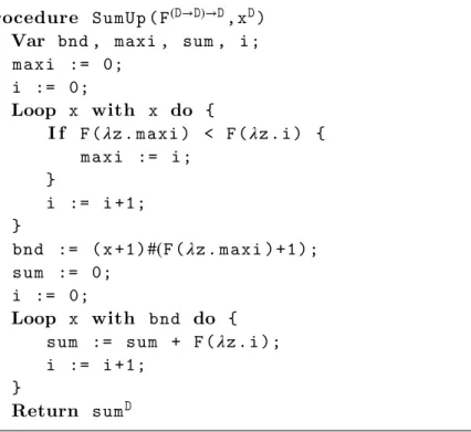
An example BTLP procedure is provided in Figure 4. This example procedure SumUp is directly sourced from [IKR02] and is an order 3 procedure that computes the function:
𝐹 , 𝑥↦∑𝑖<|𝑥|𝐹(𝜆𝑧.𝑖). It first computes a bound bnd on the result by finding the number i for which 𝐹 (𝜆𝑧.𝑖) is maximal and then computes the sum itself. Note that this procedure uses a conditional statement (If ) not included in the grammar but that can be simulated in BTLP (see [IKR02]). Such a conditional will be explicitly added to the syntax of IBTLP procedures in Definition 5.3.
Let the size of an argument be the number of syntactic elements in it. The size of input arguments is the sum of the size of the arguments in the input.
Definition 4.2 (Time complexity). For a given procedure 𝑃 of parameters (𝑣𝜏1
1,… , 𝑣
𝜏𝑛 𝑛 ), we
𝜏1× … × 𝜏𝑛 returns the maximal number of assignments executed during the evaluation of the procedure in the size of the input.
We are now ready to provide a definition of Basic Feasible Functionals at any order. Definition 4.3 (bff𝑖). For any 𝑖≥ 1, bff𝑖 is the class of order 𝑖 functionals computable by
a BTLP procedure2.
It was demonstrated in [IRK01] that bff1 = FPtime and bff2=bff.
4.2. Safe Feasible Functionals. Now we restrict the domain of bff𝑖 classes to inputs in
bff𝑘 for 𝑘 < 𝑖, the obtained classes are named sff for Safe Feasible Functionals.
Definition 4.4 (sff𝑖). sff1 is defined to be the class of order 1 functionals computable by BTLP a procedure and, for any 𝑖≥ 1, sff𝑖+1is the class of order 𝑖 + 1 functionals computable by BTLP a procedure on the input domain sff𝑖. In other words,
sff1 =bff1,
sff𝑖+1 =bff𝑖+1↾sff𝑖, ∀𝑖, 𝑖≥ 1.
This is not a huge restriction since we want an arbitrary term of a given complexity class at order 𝑖 to compute over terms that are already in classes of the same family at order 𝑘, for 𝑘 < 𝑖. Consequently, programs can be built in a constructive way component by component. Another strong argument in favor of this domain restriction is that the partial evaluation of a functional at order 𝑖 will, at the end, provide a function in ℕ ⟶ ℕ that is shown to be in bff1 (=FPtime).
5. A characterization of safe feasible functionals of any order In this section, we show our main characterization of safe feasible functionals:
Theorem 5.1. For any order 𝑖 ≥ 0, the class of functions in fp𝑖+1 over fp𝑘, 𝑘 ≤ 𝑖, is
exactly the class of functions in sff𝑖+1, up to an isomorphism. In other words, sff𝑖+1≡ fp𝑖+1↾(∪𝑘≤𝑖fp𝑘),
for all 𝑖≥ 0, up to an isomorphism.
Proof. For a fixed 𝑖, the theorem is proved in two steps: Soundness, Theorem 5.2, and Completeness, Theorem 5.14. Soundness consists in showing that any term 𝙼 whose inter-pretation is bounded by an order 𝑖 polynomial, computes a function in sff𝑖. Completeness
consists in showing that any BTLP procedure 𝑃 of order 𝑖 can be encoded by a term 𝙼 computing the same function and admitting a polynomial interpretation of order 𝑖.
Notice that functions in sff𝑖+1 return the dyadic representation of a natural number. Consequently, the isomorphism is used on functions in fp𝑖 to illustrate that a function of
type ℕ → (ℕ → ℕ) and order 1 is isomorphic to a functional of type ℕ → ℕ and of the same order using decurryfication and pair encoding over ℕ. In order to simplify the treatment we will restrict ourselves to functional terms computing functionals that are terms of type 𝚃 ⟶ b, with b ∈ B, in the remaining of the paper.
2As demonstrated in [IKR02], all types in the procedure can be restricted to be of order at most 𝑖 without
5.1. Soundness. The soundness means that any term whose interpretation is bounded by an order 𝑖 polynomial belongs to sff𝑖. For that, we will show that the interpretation allows
us to bound the computing time with an higher order polynomial.
Theorem 5.2. Any functional term 𝙼 whose interpretation is bounded by an order 𝑖 polyno-mial, computes a functional in sff𝑖.
Proof. For order 1, consider that the term 𝙼 has an interpretation bounded by a polynomial
𝑃1. For any value 𝚟, we have, by Corollary 3.10, that the computing time of 𝙼 on input 𝚟 bounded by ⦇𝙼 𝚟⦈𝜌. Consequently, using Lemma 3.12, we have that:
⦇𝙼 𝚟⦈𝜌= ⦇𝙼⦈𝜌⦇𝚟⦈𝜌= ⦇𝙼⦈𝜌(|𝚟|) ≤ 𝑃1(|𝚟|). Hence 𝙼 belongs to FPtime = sff1.
Now, for higher order, let 𝙼 be an order 𝑖 + 1 term of interpretation ⦇𝙼⦈𝜌. There exists an
order 𝑖 + 1 polynomial 𝑃𝑖+1 such that⦇𝙼⦈𝜌≤ 𝑃𝑖+1. We know that on input 𝙽, 𝙼 normalizes in
𝑂(⦇𝙼 𝙽⦈𝜌), by Corollary 3.11. Since 𝙽 computes a functional J𝙽K ∈ sff𝑖there is a polynomial
𝑃𝑖 such that ⦇𝙽⦈𝜌 ≤ 𝑃𝑖, by induction on the order 𝑖. Consequently, we obtain that the maximal number of reduction steps is bounded polynomially in the input size by:
⦇𝙼 𝙽⦈𝜌 = ⦇𝙼⦈𝜌⦇𝙽⦈𝜌≤ 𝑃𝑖+1◦𝑃𝑖,
that is, by a polynomial 𝑄𝑖+1 of order 𝑖 + 1 defined by 𝑄𝑖+1 = 𝑃𝑖+1◦𝑃𝑖.
The above result holds for terms over arbitrary basic inductive types, by considering that each value on such a type encodes an integer value.
5.2. Completeness. To prove that all functions computable by a BTLP program of order
𝑖can be defined as terms admitting a polynomial interpretation, we proceed in several steps: (1) We show that it is possible to encode each BTLP procedure 𝑃 into an intermediate procedure ❲𝑃 ❳ of a language called IBTLP (See Figure 5) for If-Then-Else Bounded Typed Loop Program such that❲𝑃 ❳ computes the same function as 𝑃 using the same number of assignments (i.e. with the same time complexity).
(2) We show that we can translate each IBTLP procedure❲𝑃 ❳ into a flat IBTLP procedure ❲𝑃 ❳, i.e. a procedure with no nested loops and no procedure calls.
(3) Then we transform the flat IBTLP procedure ❲𝑃 ❳ into a “local” and flat IBTLP procedure [❲𝑃 ❳]∅ checking bounds locally in each assignment instead of checking it globally in each loop. For that purpose, we use a polynomial time computable operator of the IBTLP language called 𝚌𝚑𝚔𝚋𝚍. The time complexity is then asymptotically preserved.
(4) Finally, we compile the IBTLP procedure [❲𝑃 ❳]∅ into a term of our language and we use completeness for first order function to show that there is a term computing the same function and admitting a polynomial interpretation. This latter transformation does not change the program behaviour in terms of computability and complexity, up to a O, but it makes the simulation by a functional program easier as each local assignment can be simulated independently of the context.
The 3 first steps just consist in transforming a BTLP procedure into a IBTLP procedure in order to simplify the compilation procedure of the last step. These steps can be subsumed as follows:
𝐼 𝑃 ∶∶= 𝑣𝜏1×…×𝜏𝑛→𝙳(𝑣𝜏1 1,… , 𝑣 𝜏𝑛 𝑛){𝐼𝑃∗𝐼 𝑉 𝐼 𝐼∗} ret 𝑣𝙳𝑟 𝐼 𝑉 ∶∶= var 𝑣𝙳 1,… , 𝑣 𝙳 𝑛; 𝐼 𝐼 ∶∶= 𝑣𝙳∶= 𝐼𝐸𝙳; | loop 𝑣𝙳 0 {𝐼𝐼 ∗}| if 𝑣𝙳 { 𝐼𝐼∗} [else { 𝐼𝐼∗}]| (𝐼𝐼∗) 𝑣𝙳 𝐼 𝐸 ∶∶= 0| 1 | 𝑣𝙳 | 𝑣𝙳0+ 𝑣𝙳1 | 𝑣𝙳0− 𝑣1𝙳 | 𝑣𝙳0#𝑣𝙳1 | 𝑣𝜏1×…×𝜏𝑛→𝙳(𝐼𝐴𝜏1 1,… , 𝐼𝐴 𝜏𝑛 𝑛) | 𝑣𝙳0× 𝑣𝙳1 | 𝚌𝚞𝚝(𝑣𝙳) | 𝚌𝚑𝚔𝚋𝚍(𝐸, 𝑋) 𝐼 𝐴∶∶= 𝑣| 𝜆𝑣1,… , 𝑣𝑛.𝑣(𝑣1′ … , 𝑣′𝑚) with 𝑣 ∉ {𝑣1,… , 𝑣𝑛} Figure 5: IBTLP grammar
Program 𝑃 ❲𝑃 ❳ ❲𝑃 ❳ [❲𝑃 ❳]∅ 𝚌𝚘𝚖𝚙([❲𝑃 ❳]∅)
Language BTLP IBTLP IBTLP IBTLP
❲❳ flat local compile
For each step, we check that the complexity in terms of reduction steps is preserved and that the transformed program computes the same function.
5.2.1. From BTLP to IBTLP.
Definition 5.3 (IBTLP). A If-Then-Else Bounded Typed Loop Program (IBTLP) is a non-recursive and well-formed procedure defined by the grammar of Figure 5.
The well-formedness assumption and variable bounds are the same as for BTLP. In a loop statement, the guard variable 𝑣0 still cannot be assigned to within 𝐼 𝐼∗. A IBTLP procedure
𝐼 𝑃 has also a time complexity 𝑡(𝐼𝑃 ) defined similarly to the one of BTLP procedures. The main distinctions between an IBTLP procedure and a BTLP procedure are the following:
∙ there are no loop bounds in IBTLP loops. Instead loop bounds are written as instruction annotations: a IBTPL loop (loop 𝑣𝙳
0 {𝐼𝐼 ∗})
𝑣𝙳 corresponds to a BTLP instruction of the
shape
Loop 𝑣𝙳
0 with 𝑣
𝙳 do {𝐼𝐼∗}. ∙ IBTLP includes a conditional statement if 𝑣𝙳 { 𝐼𝐼∗
1 } else { 𝐼𝐼 ∗
2} evaluated in a standard way: if variable 𝑣 is 0 then it is evaluated to 𝐼𝐼2∗. In all other cases, it is evaluated to 𝐼 𝐼1∗, the else branching being optional.
∙ IBTLP includes a basic operator × such that 𝑥 × 𝑦 = 2|𝑥|+|𝑦|.
∙ IBTLP includes a unary operator 𝚌𝚞𝚝 which removes the first character of a number (i.e. 𝚌𝚞𝚝(0) = 0, 𝚌𝚞𝚝(2𝑥 + 𝑖) = 𝑥 where 𝑖 ∈ {0, 1}).
∙ IBTLP includes an operator 𝚌𝚑𝚔𝚋𝚍 computing the following function: 𝚌𝚑𝚔𝚋𝚍(𝐸, 𝑋) =
{
J𝐸 K, if|J𝐸 K| ≤ |𝑥|, 𝑥 ∈ 𝑋 ,
0, otherwise,
whereJ𝐸 K is the dyadic number obtained after the evaluation of expression 𝐸 and 𝑋 is a finite set of variables.
Notice that 𝚌𝚑𝚔𝚋𝚍 is in sff1 provided that the input 𝐸 is computable in polynomial time and both × and cut are in sff1. The semantics of an IBTLP procedure is also similar to the one of a BTLP procedure: during the execution of an assignment, the bound check is performed on instruction annotations instead of being performed on loop bounds. However IBTLP is strictly more expressive than BTLP from an extensional perspective: a loop can be unbounded. This is the reason why only IBTLP procedures obtained by well-behaved transformation from BTLP procedures will be considered in the remainder of the paper.
Now we define a program transformation❲.❳ from BTLP to IBTLP. For each loop of a BTLP program, this transformation just consists in recording the variable appearing in the with argument of a contextual loop and putting it into an instruction annotation as follows: ❲Loop 𝑣𝙳 0 with 𝑣 𝙳 1 do {𝐼 ∗}❳ = (loop 𝑣𝙳 0 {❲𝐼❳ ∗}) 𝑣𝙳 1.
Any assignment is left unchanged and this transformation is propagated inductively on procedure instructions so that any inner loop is transformed. We denote by ❲𝑃 ❳ the IBTLP procedure obtained from the BTLP procedure 𝑃 . Hence the following lemma straightforwardly holds:
Lemma 5.4. Given a procedure 𝑃 , let J𝑃 K denote the function computed by 𝑃 . For any BTLP procedure 𝑃 , we have J𝑃 K = J❲𝑃 ❳K and 𝑡(𝑃 ) = 𝑡(❲𝑃 ❳).
Proof. The transformation is semantics-preserving (the computed function is the same). Any assignment in 𝑃 corresponds to exactly one assignment in❲𝑃 ❳ and the number of iterations of the loop instructions Loop 𝑣 with … and loop 𝑣 are both in|𝑣|.
5.2.2. From IBTLP to Flat IBTLP.
Definition 5.5 (Flat IBTLP). A If-Then-Else Bounded Typed Loop Program (IBTLP) is flat if it does not contain nested loops.
We will show that it is possible to translate any IBTLP procedure into a Flat IBTLP procedure using the if construct.
There are only three patterns of transformation: (1) one pattern for nested loops, called Unnest, (2) one pattern for sequential loops, called Unseq,
(3) and one for procedure calls inside a loop, called Unfold, that we describe below:
(1) The first transformation Unnest consists in removing a nested loop of a given procedure. Assume we have a IBTLP procedure with two nested loops:
( l o o p x { 𝐼 𝐼1∗ ( l o o p y {𝐼 𝐼2∗})𝑧 𝐼 𝐼3∗})w. We can translate it to a IBTLP procedure as:
t o t a l := w×y ; dx := 1; gt := t o t a l ; gy := y ; lb := x# t o t a l ; l o o p lb { if dx {(𝐼 𝐼1∗)w} if gy {((𝐼 𝐼2∗)z)w gy := cut ( gy );} if dx { dx := 0; (𝐼 𝐼3∗)w}
if gt { gt := cut ( gt );}
e l s e { gt := t o t a l ; gy := y ; dx := 1;} }
where all the variables dx, total, gt, gy and lb are fresh local variables and 𝐼𝐼1∗, 𝐼 𝐼2∗ and 𝐼 𝐼3∗ are instructions with no loop. The intuition is that variables dx and gy tell whether the loop should execute 𝐼 𝐼1∗ and 𝐼 𝐼2∗ respectively. Variable gt counts the number of times to execute the sub-loop.
(2) The second transformation Unseq consists in removing two sequential loops of a given procedure. Assume we have a IBTLP procedure with two sequential loops:
( l o o p x1 {𝐼 𝐼1∗})w
1 𝐼 𝐼
∗
2 ( l o o p x3 {𝐼 𝐼3∗})w3.
We can translate it to a single loop IBTLP procedure as: gx := x1 ; dy := 1; lb := x1×x3; l o o p lb { if gx { gx := cut gx ; (𝐼 𝐼1∗)w1} e l s e { if dy {𝐼 𝐼2∗} e l s e { dy := 0; (𝐼 𝐼3∗)w3} } }
where gx, dy and lb are fresh local variables and 𝐼𝐼1∗, 𝐼 𝐼2∗ and 𝐼 𝐼3∗ are instructions with no loop.
(3) The last transformation Unfold consists in removing one procedure call of a given procedure. Assume we have a IBTLP procedure with a call to procedure 𝑃 of arity 𝑛:
𝑋 := 𝑃 (𝐼 𝐴1, ..., 𝐼 𝐴𝑛);
We can translate it to a computationally equivalent IBTLP procedure after removing the call to procedure 𝑃 . For that purpose, we carefully alpha-rename all the variables of the procedure declaration (parameters and local variables) to obtain the procedure
𝑃(𝑣1,… , 𝑣𝑛){𝐼𝑃∗𝐼 𝑉 𝐼 𝐼∗} ret 𝑣
𝑟 then we add the procedure declarations 𝐼 𝑃∗ to the
caller procedure list of procedure declarations, and the local variables 𝐼 𝑉 and parameters
𝑣1,… , 𝑣𝑛 to the caller procedure list of local variable declarations and then we generate the following code:
𝑣1 := 𝐼 𝐴1; … 𝑣𝑛 := 𝐼 𝐴𝑛; 𝐼 𝐼∗ 𝑋 := 𝑣𝑟;
This program transformation can be extended straightforwardly to the case where the procedure call is performed in a general expression. Notice that unfolding a procedure is necessary as nested loops may appear because of procedure calls.
These three patterns can be iterated on a IBTLP procedure (from top to bottom) to obtain a Flat IBTLP procedure in the following way:
Definition 5.6. The transformation 𝐼 𝑃 is a mapping from IBTLP to IBTLP defined by:
𝐼 𝑃 = (Unnest!◦Unseq!)!◦Unfold!(𝐼𝑃 ),
where, for a given function f, 𝑓! is the least fixpoint of 𝑓 on a given input and◦ is the usual mapping composition.
[𝑣𝜏1×…×𝜏𝑛→𝙳(𝑣𝜏1 1,… , 𝑣 𝜏𝑛 𝑛)𝐼𝑃∗ 𝐼 𝑉 𝐼 𝐼∗ ret 𝑣𝙳𝑟]𝑋 = 𝑣𝜏1×…×𝜏𝑛→𝙳(𝑣 𝜏1 1,… , 𝑣 𝜏𝑛 𝑛)𝐼𝑃∗ 𝐼 𝑉 [𝐼𝐼]∗𝑋 ret 𝑣𝑟 [𝐼𝐼𝑣]𝑋 = [𝐼𝐼]𝑋∪{𝑣}
[if 𝑣𝙳 { 𝐼𝐼1∗ } else { 𝐼𝐼2∗}]𝑋 = if 𝑣𝙳 { [𝐼𝐼1]∗𝑋 } else { [𝐼𝐼2]∗𝑋}
[loop 𝑣𝙳0{𝐼𝐼∗}; ]𝑋 = loop 𝑣𝙳0 {[𝐼𝐼]∗𝑋}
[𝑣𝙳∶= 𝐼𝐸; ]𝑋 = 𝑣𝙳∶= 𝚌𝚑𝚔𝚋𝚍(𝐼𝐸𝙳, 𝑋);
Figure 6: From Flat IBTLP to Local and Flat IBTLP
Notice that this procedure is polynomial time computable as each application of a call to Unfold consumes a procedure call (and procedures are non recursive) and each application
of an Unnest or Unseq call consumes one loop. Consequently, fixpoints always exist. Lemma 5.7. For any BTLP procedure 𝑃 , ❲𝑃 ❳ is a flat IBTLP procedure.
Proof. First notice that repeated application of the Unfold pattern may only introduce a constant number of new loops as procedures are non-recursive. Consequently, the fixpoint Unfold! is defined and reached after a constant number (in the size of the procedure) of applications. Each application of a Unseq pattern or Unnest pattern decreases by one the number of loop within a procedure. Consequently, a fixpoint is reached (modulo 𝛼-equivalence) and the only programs for which such patterns cannot apply are programs with a number of loops smaller than 1.
Lemma 5.8. For any BTLP procedure 𝑃 , we have J❲𝑃 ❳K = J𝑃 K and 𝑡(❲𝑃 ❳) = 𝑂(𝑡(𝑃 )). Proof. In the first equality, the computed functions are the same since the program trans-formation preserves the extensional properties. For the second equality, the general case can be treated by a structural induction on the procedure ❲𝑃 ❳. For simplicity, we con-sider the case of a procedure ❲𝑃 ❳ only involving 𝑛 nested loops over guard variables
𝑥1,… , 𝑥𝑛 and loop bounds 𝑥𝑛+1,… , 𝑥2𝑛, respectively over one single basic instruction (e.g. one assignment with no procedure call). With inputs of size 𝑚, this procedure will have a worst case complexity of 𝑚𝑛 (when the loop bounds are not reached). Consequently,
𝑡(𝑃 )(𝑚) = 𝑚𝑛. This procedure will be transformed into a flat IBTLP procedure using the
Unnest transformation 𝑛 − 1 times over a variable 𝑧 containing the result of the computation
𝑥1#((𝑥2× 𝑥𝑛+1)#(… 𝑥3× 𝑥𝑛+2)#(𝑥𝑛× 𝑥2𝑛) …) as initial value. Consequently, on an input of size
𝑚, we have 𝑡(❲𝑃 ❳)(𝑚) ≤ |𝑧| = |𝑥1| × (|𝑥2| + |𝑥𝑛+1|) × … × (|𝑥𝑛| + |𝑥2𝑛|) ≤ 2𝑛−1× 𝑚𝑛 = 𝑂(𝑚𝑛),
as for each 𝑖 |𝑥𝑖| ≤ 𝑚 and by definition of the # and × operators. We conclude using
Lemma 5.4.
5.2.3. From Flat IBTLP to Local and Flat IBTLP. Now we describe the last program transformation [−]𝑋 that makes the check bound performed on instruction annotations explicit. For that purpose, [−]𝑋 makes use of the operator 𝚌𝚑𝚔𝚋𝚍 and records a set of variables
𝑋 (the annotations enclosing the considered instruction). The procedure is described in Figure 6. Notice that the semantics condition ensuring that no assignment must be performed on a computed value of size greater than the size of the loop bounds for a BTLP procedure or than the size of the loop annotations for a IBTLP procedure has been replaced by a local
𝚌𝚘𝚖𝚙(𝑣(𝑣1,… , 𝑣𝑚) 𝐼𝑃∗var 𝑣𝑚+1,… , 𝑣𝑛; 𝐼𝐼∗ ret 𝑣𝑟) = 𝜆𝑠.𝜋𝑟𝑛(𝚌𝚘𝚖𝚒 𝑛(𝐼𝐼∗ ) 𝑠) 𝚌𝚘𝚖𝚒𝑛(𝐼𝐼1 … 𝐼𝐼𝑘) = 𝚌𝚘𝚖𝚒𝑛(𝐼𝐼𝑘) … 𝚌𝚘𝚖𝚒𝑛(𝐼𝐼1) 𝚌𝚘𝚖𝚒𝑛(𝑣𝑖 ∶= 𝐼𝐸; ) = 𝜆⟨𝑣1,… , 𝑣𝑛⟩.⟨𝑣1,… , 𝑣𝑖−1, 𝚌𝚘𝚖𝚎(𝐼 𝐸), 𝑣𝑖+1,… , 𝑣𝑛⟩ 𝚌𝚘𝚖𝚒𝑛(loop 𝑣𝑖 {𝐼𝐼∗}) = 𝜆⟨𝑣 1,… , 𝑣𝑛⟩.( ( 𝚕𝚎𝚝𝚁𝚎𝚌 𝑓 = 𝜆̃𝑡.𝜆𝑠.𝚌𝚊𝚜𝚎 ̃𝑡 𝚘𝚏 0 → 𝑠 𝑗(𝑡) → 𝑓 𝑡(𝚌𝚘𝚖𝚒𝑛(𝐼𝐼∗) 𝑠) ) 𝑣𝑖) 𝚌𝚘𝚖𝚒𝑛(if 𝑣𝙳𝑖 { 𝐼𝐼∗ 1 } else { 𝐼𝐼 ∗ 2}) = 𝜆⟨𝑣1,… , 𝑣𝑛⟩.𝚌𝚊𝚜𝚎 𝑣𝑖 𝚘𝚏 0 → 𝚌𝚘𝚖𝚒𝑛(𝐼𝐼2∗)| 𝑗(𝑡) → 𝚌𝚘𝚖𝚒 𝑛(𝐼𝐼∗ 1) with 𝑗 ∈ {0, 1} 𝚌𝚘𝚖𝚎(𝑐) = 𝑐, 𝑐∈ {1, 𝑣𝙳} 𝚌𝚘𝚖𝚎(𝑣𝙳0 𝚘𝚙 𝑣𝙳1) = 𝚘𝚙 𝑣0𝑣1, 𝚘𝚙 ∈ {+, −, #, ×} 𝚌𝚘𝚖𝚎(𝚌𝚞𝚝(𝑣𝙳)) = 𝚌𝚞𝚝 𝑣 𝚌𝚘𝚖𝚎(𝚌𝚑𝚔𝚋𝚍(𝐼 𝐸, {𝑣𝑗 1,… , 𝑣𝑗𝑟})) = 𝚌𝚑𝚔𝚋𝚍 𝚌𝚘𝚖𝚎(𝐼𝐸) (⊓ 𝙳 𝑟 𝑣𝑗1 … 𝑣𝑗𝑟) 𝚌𝚘𝚖𝚎(𝑣(𝐼 𝐴1,… , 𝐼𝐴𝑛)) = 𝑣 𝚌𝚘𝚖𝚎(𝐼𝐴1) … 𝚌𝚘𝚖𝚎(𝐼𝐴𝑛) 𝚌𝚘𝚖𝚎(𝜆𝑣1,… , 𝑣𝑛.𝑣(𝑣′1… , 𝑣 ′ 𝑚)) = 𝜆𝑣1.… 𝜆𝑣𝑛.(… (𝑣 𝑣′1) … 𝑣 ′ 𝑚) …)
Figure 7: Compiler from Local and Flat IBTLP to terms
computation performing exactly the same check using the operator 𝚌𝚑𝚔𝚋𝚍. Consequently, we have:
Lemma 5.9. For any BTLP procedure 𝑃 , we have J[❲𝑃 ❳]∅K = J𝑃 K and 𝑡([❲𝑃 ❳]∅) = 𝑂(𝑡(𝑃 )). Proof. We use Lemma 5.8 together with the fact that extensionality and complexity are both preserved.
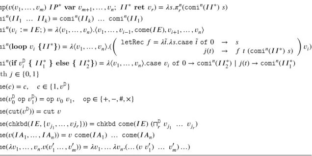
5.2.4. From Local and Flat IBTLP to terms. We then encode Flat and Local IBTLP in our functional language. For this, we define a procedure 𝚌𝚘𝚖𝚙 that will “compile” IBTLP procedures into terms. For that purpose, we suppose that the target term language includes constructors for numbers (0 and 1), a constructor for tuples ⟨…⟩, all the operators of IBTLP as basic prefix operators (+, -, #, …), min operators ⊓𝙳
𝑛 computing the min of the
sizes of 𝑛 dyadic numbers and a 𝚌𝚑𝚔𝚋𝚍 operator of arity 2 such thatJ𝚌𝚑𝚔𝚋𝚍K(𝙼, 𝙽) = J𝙼K if |J𝙼K| ≤ |J𝙽K| (and 0 otherwise). All these operators are extended to be total functions in the term language: they return 0 on input terms for which they are undefined. Moreover, we also require that the Flat and Local IBTLP procedures given as input are alpha renamed so that all parameters and local variables of a given procedure have the same name and are indexed by natural numbers. The compiling process is described in Figure 7, defining 𝚌𝚘𝚖𝚙, 𝚌𝚘𝚖𝚒𝑛, 𝚌𝚘𝚖𝚎 that respectively compile procedures, instructions and expressions. The
𝚌𝚘𝚖𝚒 compiling process is indexed by the number of variables in the program 𝑛.
For convenience, let 𝜆⟨𝑣1,… , 𝑣𝑛⟩. be a shorthand notation for 𝜆𝑠.𝚌𝚊𝚜𝚎 𝑠 𝚘𝚏 ⟨𝑣1,… , 𝑣𝑛⟩ →
and let 𝜋𝑛
𝑟 be a shorthand notation for the r-th projection 𝜆⟨𝑣1,… , 𝑣𝑛⟩.𝑣𝑟.
The compilation procedure works as follows: any Local and Flat IBTLP procedure of the shape 𝑣(𝑣1,… , 𝑣𝑚) 𝐼𝑃∗ var 𝑣𝑚+1,… , 𝑣𝑛; 𝐼𝐼∗ ret 𝑣𝑟 will be transformed into a term
of type 𝜏1× … × 𝜏𝑛 → 𝜏𝑟, provided that 𝜏𝑖 is the type of 𝑣𝑖 and that 𝜏1 × … × 𝜏𝑛 is the type for n-ary tuples of the shape⟨𝑣1,… , 𝑣𝑛⟩. Each instruction within a procedure of type