Quantitative evaluation of linear and nonlinear methods characterizing interdependencies between brain signals.

HAL Id: inserm-00129780

https://www.hal.inserm.fr/inserm-00129780

Submitted on 14 Feb 2007

HAL is a multi-disciplinary open access

archive for the deposit and dissemination of sci-entific research documents, whether they are pub-lished or not. The documents may come from teaching and research institutions in France or

L’archive ouverte pluridisciplinaire HAL, est destinée au dépôt et à la diffusion de documents scientifiques de niveau recherche, publiés ou non, émanant des établissements d’enseignement et de recherche français ou étrangers, des laboratoires

Quantitative evaluation of linear and nonlinear methods

characterizing interdependencies between brain signals.

Karim Ansari-Asl, Lotfi Senhadji, Jean-Jacques Bellanger, Fabrice Wendling

To cite this version:

Karim Ansari-Asl, Lotfi Senhadji, Jean-Jacques Bellanger, Fabrice Wendling. Quantitative evaluation of linear and nonlinear methods characterizing interdependencies between brain signals.. Physical Review E : Statistical, Nonlinear, and Soft Matter Physics, American Physical Society, 2006, 74 (3 Pt 1), pp.031916. �10.1103/PhysRevE.74.031916�. �inserm-00129780�

Quantitative evaluation of linear and nonlinear methods characterizing

interdependencies between brain signals

Karim Ansari-Asl 1,2 ,Lotfi Senhadji1,2, Jean-Jacques Bellanger1,2,Fabrice Wendling1,2

1 INSERM, U642, Rennes, F-35000, France; 2 Université de Rennes 1, LTSI, Rennes, F-35000, France.

July 2006

Correspondence: Lotfi Senhadji

LTSI, Campus de Beaulieu, Université de Rennes 1, 263 Avenue du Général Leclerc - CS 74205 - 35042 Rennes Cedex, France. Tel: (33) 2 23 23 62 20

Fax: (33) 2 23 23 69 17

Email: lotfi.senhadji@univ-rennes1.fr

HAL author manuscript inserm-00129780, version 1

HAL author manuscript

Abstract

Brain functional connectivity can be characterized by the temporal evolution of correlation between signals recorded from spatially-distributed regions. It is aimed at explaining how different brain areas interact within networks involved during normal (as in cognitive tasks) or pathological (as in epilepsy) situations. Numerous techniques were introduced for assessing this connectivity. Recently, some efforts were made to compare methods performances but mainly qualitatively and for a special application. In this paper, we go further and propose a comprehensive comparison of different classes of methods (linear and nonlinear regressions, phase synchronization (PS), and generalized synchronization (GS)) based on various simulation models. For this purpose, quantitative criteria are used: in addition to mean square error (MSE) under null hypothesis (independence between two signals) and mean variance (MV) computed over all values of coupling degree in each model, we introduce a new criterion for comparing performances. Results show that the performances of the compared methods are highly depending on the hypothesis regarding the underlying model for the generation of the signals. Moreover, none of them outperforms the others in all cases and the performance hierarchy is model-dependent.

I. INTRODUCTION

Brain functional connectivity is defined as the way different brain areas interact within networks involved during normal (as in cognitive tasks) or pathological (as in epilepsy) activity. It can be characterized by the temporal evolution of the cross-correlation (in a wide sense) between signals recorded from spatially-distributed regions. During the past decades, numerous techniques have been introduced for measuring this correlation. In the early fifties, the first developed methods [1] were based on the cross-correlation function and its counterpart in the frequency domain, i.e., the coherence function [2, 3] just after fast Fourier transform (FFT) algorithms were introduced [4]. Some other methods based on a similar concept but using time-varying linear models to estimate the cross-correlation were introduced later and were used to characterize the relationship between brain oscillations in the time and/or frequency domain [5, 6].

As aforementioned methods are mostly linear, recently a considerable number of studies have been dedicated to the development of nonlinear methods [7], mostly because of the nonlinear nature of mechanisms at the origin of EEG signals. A family of methods based on mutual information [8] or on nonlinear regression [9, 10] was first introduced in the EEG field. Another family is currently developing, based on works related to the study of nonlinear dynamical systems and chaos [11, 12]. The latter family can be divided into two groups: (i) phase synchronization (PS) methods [13, 14] which first estimate the instantaneous phase of each signal and then compute a quantity based on co-variation of extracted phases to determine the degree of relationship; (ii) generalized synchronization (GS) methods [15, 16] which also consist of two steps, in the first one, state space trajectories are reconstructed from scalar time series signals and in the second one, an index of similarity is computed to quantify the similarity between these trajectories.

Given the number and the variety of methods introduced for characterizing brain signal interactions and considering the diversity of situations in which these methods are applied, there is a need for identifying objectively, among available methods, those which offer the best performances.

Recently, some efforts have been made for comparing methods but mainly qualitatively [17, 18] and for particular applications [19, 20].

In this paper, we go further and propose a comprehensive comparison of the aforementioned classes of methods (linear and nonlinear regression, phase synchronization, and generalized synchronization) based on various simulation models (linearly correlated noises, nonlinear coupled oscillators and coupled neuronal population models) in which a coupling parameter can be tuned. Methods are compared according to quantitative criteria: (i) the mean square error (MSE) under null hypothesis (independence between the two analyzed signals); (ii) the mean variance (MV) computed over all values of the coupling parameter in each model; (iii) in addition to two preceding criteria, we proposed a new criterion related to the method sensitivity.

The paper is organized as follows: Section II introduces simulation models and briefly reviews some of the methods widely used in the field of EEG to estimate the degree of relationship between two signals. Results are presented in Section III and discussed in Section IV.

II. METHODS A. MODELS

In this section general features of models considered in this study are introduced. Each of them is a more or less simplified version of a general finite dimensional state-space model with three inputs and two outputs. This general model denoted by C_,

X Y

M is decomposed in two sub-systems S1 and

S2 as illustrated in Fig. 1. To describe state evolution (on discrete time or on continuous time) of the

global system two finite dimensional marginal state vectors, respectively denoted and Y , must

be introduced. In an EEG measurement perspective, and Y macroscopically represent

dynamical states of two functionally interdependent neuronal subpopulations, respectively. Each subsystem is specified by a state evolution equation:

X X

(

)

(

)

( ) ( ); ( ), , ( ) ( ) ( ); ( ), , ( ) C m C n X t F X t v t t X t Y t G Y t w t t Y t τ τ τ θ θ τ τ θ θ τ ⎧ + = ≤ ≤ + ∈ ⎪ ⎨ _{+ = ≤ ≤ + ∈} ⎪⎩

where matrix is a matrix of positive numbers interpreted in the sequel as a coupling

parameter which weights the effect of "non-autonomous" terms v and w respectively on states and Y (Fig. 1).

(

i j, C= C

)

X

The inputs N1, N2, and N3 are mutually independent, zero-memory, zero-mean and unit-variance

stochastic processes (white noises) which can be interpreted, in a physiological perspective, as influences from distant neural populations. Input N3 corresponds to a possible shared afference. The

scalar outputs x and , in the same perspective, correspond to two EEG channels. If it exists, the dynamical ‘coupling’ between states and Y is represented through a functional dependence of v on Y and on the shared input N

y

X

3 and through the dependence of w on X and N3:

( )

( )

( )

(

)

( )

( )

( )

(

)

1 1,1 1 3 2 2,1 2 3 ( ) , , , ( ) , , , v t g C N t N t Y t w t g C N t N t X t ⎧ = ⎪ ⎨ = ⎪⎩ .

The models for the two output scalar signals are:

( )

(

( ) ( )

( )

)

( )

21

(

( ) ( )

12

( )

)

, , , , x t h X t Y t m t y t h X t Y t m t ⎧ = ⎪ ⎨ = ⎪⎩ 1

g , , and are deterministic functions. The measurement noises, if present, are modeled by

two independent random processes and .

2

g h₁ h₂

1( )

m t m t₂( )

If v does not depend on Y(.) and w does not depend on X(.) and if furthermore N3 = 0, then the

two subsystems S1 and S2 are disconnected. In this case and when inputs N1 and N2 are present,

outputs x and are statically independent if (resp. ) is not a function of Y (resp. ) . Then

equations become

y h₁ h₂ X

( )

1

(

( )

)

x t =h X t and y t

( )

=h Y t2

(

( )

)

, in absence of measurement noise.

The dashed lines in Fig. 1 correspond to the influences of S2 on the signal x . These influences are

not considered in the present study (neither a feedback influence of X on Y nor a forward

influence of Y on x ) except for one model (the model denoted by M1 here after). This

consideration corresponds to a causal influence directed from S1 to S2 and clearly does not address

the most general bidirectional situation which is beyond the scope of this paper. Consequently, matrix C is the parameter which tunes the dependence of on . When C is null no dependence exists. Dependence between the two systems is expected to increase with C coefficients. Depending on model type, for large values of these coefficients and when N

y X

2=0 and m2=0, output becomes a

deterministic function of state and of N

y

X 3.

In order to comprehensively simulate a wide range of coupled temporal dynamics we used various mathematical models as well as a physiologically-relevant computational model of EEG simulation from coupled neuronal populations. Motivations for the choice of these kinds of relationship models in the context of brain activity are discussed in a previous work [21].

Degenerated model M1 is derived by setting C1,1 =C2,1=c and by letting the other matrix

coefficient equal to zero with x=X = and y Y wv = = . This model generates two broadband

signals (x y, ) from the mixing of the two independent white noises (N1, N2) with the common noise

(N3):

(

)

(

)

1 3 2 3 1 1 x c N cN y c N cN = − + = − +

where 0≤c≤1 is the coupling degree; for c=0 the signals are independent and for they are identical.

1

c=

In model M2, the general description above reduces to: v=N1, w=N2, x=h X1

( )

, C2,3 =c, and

. The other coefficients of the matrix C are all equal to zero. In practice, four low-pass filtered white noises (NF

(

2 , ,

y=h X Y c

)

1, NF2, NF3, and NF4) are combined in two ways to generate two

narrowband signals around a frequency f₀. Generated signals share either a phase relationship (PR) or an amplitude relationship (AR), only:

(

)

(

)

(

)

(

)

(

)

(

)

(

)

1 0 1 2 0 1 2 1 0 1 1 2 0 cos 2 : cos 2 1 cos 2 : 1 cos 2 x A f t PR y A f t c c x A f t AR y cA c A f t π φ π φ φ π φ 2 π φ = + = + + − = + = + − + ⎧ ⎨ ⎩ ⎧ ⎨ ⎩ where 2 2 1 1 2 A = NF +NF , 2 2 2 3 4 A = NF +NF ,

( )

2 1 1 arctan NF NF φ = ,

( )

4 3 2 arctan NF NF φ = , and . For

, the two generated signals have independent phase and amplitude and for , they have

identical phase or amplitude.

0≤ ≤ 1c

0

c= c=1

We also evaluated interdependence measures on coupled temporal dynamics obtained from two models of coupled nonlinear oscillators, namely the Rössler [22] and Hénon [23] deterministic systems. In model M3, where two Rössler systems [24] are coupled, the driver system is

(

)

1 2 3 2 1 2 3 3 1 0.15 0.2 10 x x dx x x dt dx x x dt dx x x dt ω ω = − − = + = + −

and the response system is

(

)

(

)

1 2 3 1 1 2 1 2 3 3 1 0.15 0.2 10 y y dy y y c x y dt dy y y dt dy y y dt ω ω = − − + − = + = + −

here ω_x =0.95

,

ω_y =1.05

,

and c is the coupling degree. For this model, (other are

equal to zero), ,

2,1

C = c C_{i j,}

1 2 3 0

v=N =N =N = w=g₂

(

X c,

)

and the outputs are linear forms of the state vectors: x=h X₁( )=HX and y=h Y₂( )=HY .

In model M4, we used two Hénon maps to simulate a unidirectional coupled system. The Hénon

map [25] is a nonlinear deterministic system which is discrete by construction. Here, the driver system is

[

]

2

[ ]

[

]

1 1.4 x 1

x n+ = −x n +b x n−

and the response system is

[

]

(

[ ] [ ]

(

)

2

[ ]

)

[

]

1 1.4 1 _y 1

y n+ = − cx n y n + −c y n +b y n−

where c is a coupling degree and ; to create different situations, once is set to 0.3 to have two identical systems (M

0.3

x

b = b_y

4a) and once by is set to 0.1 to have two non-identical systems (M4b).

For each of these two cases (identical or different systems), we added some measurement noise to verify the robustness of estimators against changes in signal-to-noise ratio (S/N), here we evaluated the noise-free case (S/N=inf.) and S/N=2. S/N was computed as the ratio of standard deviation (Std) of the signal over the Std of the noise. In this case, this model matches the general description figure with C_2,1=c, v=N₁ =N₂ =N₃ =0, w=g₂

(

X c,

)

, x=h X₁( )=HX +m₁, and

.

2( ) 2

y=h Y =HY +m

Finally, to further match dynamics encountered in real EEG signals, especially in epilepsy, we considered a physiologically-relevant computational model of EEG generation from a pair of coupled populations of neurons [26]. Each population contains two subpopulations of neurons that mutually interact via excitatory or inhibitory feedback: main pyramidal cells and local interneurons. The influence from neighboring is modeled by an excitatory input p t

( )

(i.e., here or ) that globally represents the average density of afferent action potentials (Gaussian noise). Since pyramidal cells are excitatory neurons that project their axons to other areas of the brain, the model accounts for this organization by using the average pulse density of action potentials from the main cells of a first population as an excitatory input to a second population of neurons. A connection from a given population i to a population j is characterized by parameter

1

N N₂

ij

K which represents the degree of coupling associated with this connection. Other parameters include excitatory and inhibitory gains in feedback loops as well as average number of synaptic contacts between

subpopulations. Appropriate setting of parameters Kij allows for building systems where neuronal populations can be unidirectionally and/or bidirectionally coupled. In model M5, we considered the case of two populations of neurons unidirectionally coupled (K12 = is varied and c stays equal to 0). This model was used to generate two kinds of signal: background (M

21 K

5(BKG)) and spiking

(M5(SPK)) EEG activity. For both cases, normalized coupling parameter was varied from 0

(independent situation) to 1 value under which temporal dynamics of signals stay unchanged. Following the general description of the simulation model we have, C_2,1=c, v=N₁,

, ,

(

)

2 , , 2 2

w=g X c N = N +cHX N₃ =0 x=h X₁( )=HX and y=h Y₂( )=HY .Here, HX and HY are linear forms of the state vectors

B. Interdependence measures and coupled systems

In experimental context, the classical approach to evaluate a functional coupling between two systems S1 and S2 is a two steps procedure. The first step consists in building an indicator of

relationship between state vectors and Y . The second step focuses on the estimation of the indicator as a function of the two outputs

X

x and observed over a sliding window of fixed length. The window length is set so that the observed signals are locally stationary. A naïve approach is to reduce this functional coupling to the value of parameter C in a given model

y

,

C X Y

M , and hence to

restrict the characterization to an estimation of this parameter. Indeed a value of C is not a definitive answer to the problem. The link, in a given model, between this value and the joint dynamical activity of coupled systems is generally not simple to establish theoretically. However, in some particular cases it can be derived analytically (see appendix A). Even in the case where we have an

exact mathematical model C_,

X Y

M allowing to accurately simulate the joint evolution of state

vectors and Y , it can be hard to closely analyze the functional relationship between them. The difficulty is that a general definition of a functional relationship index

X

(

,

)

C X Y

r M from X to Y ,

which should be taken as an "absolute reference", does not exist (a particular definition will generally capture only some cross-dynamical features). Furthermore a theoretical definition is not sufficient. It is also necessary to make a measurement from output signals x and y, i.e., to build an

estimator of . In a model identification approach a natural estimator should be

where is an estimation of C in model

ˆ( , ) r x y r M( CX Y_, )

)

(

)

(

ˆ( )_,

)

, ˆ , C x y_{X Y} r x y =r M C x yˆ

(

, C_, X Y

M . This model based

approach is beyond the scope of this paper. Our concern here is essentially to compare various coupling functionals R x y

(

,

)

defined directly on a pair of scalar observation signals without explicit reference to an underlying model. In this study, compared functionals and corresponding estimators R x yˆ

(

,

)

are those widely used in the literature (see section II.C). These measures can be considered as descriptive methods.

C. Evaluated interdependence measures

We investigated the most widely used methods for characterizing stationary interactions between systems. These may be divided into three categories: (i) linear and nonlinear regression: Pearson correlation coefficient (R²), coherence function (CF) and nonlinear regression (h²); (ii) phase synchronization: Hilbert phase entropy (HE), Hilbert mean phase coherence (HR), wavelet phase entropy (WE) and wavelet mean phase coherence (WR); (iii) generalized synchronization: three similarity indexes (S, H, N) and synchronization likelihood (SL).

Here we review succinctly their definitions.

i) For two time series x t

( )

and , Pearson correlation coefficient is defined in the time domain as follows [27]

( )

y t

( ) (

)

(

)

( )

(

)

(

(

)

)

2 2 cov , max var var x t y t R x t y t τ τ τ + = ⋅ +

where var, cov, and τ denote respectively variance, covariance, and time shift between the two time series.

The magnitude-squared coherence function (CF) can be formulated as [28]:

( )

_{( )}

( )

_{( )}

2 2 _xy xy xx yy S f f S f S f ρ = ⋅

where S_xx

( )

f and Syy

( )

f are respectively the power spectral densities of x t

( )

and y t

( )

,

and is their cross-spectral density. It is the counterpart of R² in the frequency domain and can be interpreted as the squared modulus of a frequency-dependent complex correlation coefficient.

( )

xy

S f

Among nonlinear regression analysis methods, we chose a method introduced in the field of EEG analysis by Lopes da Silva and colleagues [29] and more recently evaluated in a model of coupled neuronal populations [30]. Based on the fitting of a nonlinear curve by piece-wise linear approximation [31], this method provides a nonlinear correlation coefficient referred to as h²:

(

) ( )

(

)

(

)

(

)

2 var / max 1 var xy y t x t h y t τ τ τ ⎛ + ⎞ = ⎜_⎜ − ⎟_⎟ + ⎝ ⎠ where

(

) ( )

(

)

(

(

)

(

( )

)

2

)

var / arg min

g

y t+τ x t E y t⎡_⎣ +τ −g x t ⎤_⎦

where g

( )

⋅ is a function which approximates the statistical relationship from x t

( )

to y t

( )

.

ii) Phase synchronization estimation consists of two steps [13]. The first step is the instantaneous

phase extraction of each signal and the second step is the quantification of the degree of synchronization via an appropriate index. Phase extraction can be done by different techniques. Two of them are used in this work: the Hilbert transform and the wavelet transform. Using the Hilbert transform, analytical signal associated to a real time series x t

( )

is derived:

( )

( )

( )

( )

( ) , H x i t H x x Z t =x t +iH ⎡_⎣x t ⎤_⎦=A t eφ

where H , H x

φ , and H

( )

x

A t are respectively the Hilbert transform, the phase, and the amplitude of

( )

x t . Complex continuous wavelet transform can also be used to estimate the phase of signal [32]:

( ) (

)( )

( ) (

)

( )

( ) _, * W x i t W x x W t = ψ x t =

∫

ψ t x t′ −t dt′ ′= A t ⋅eφ where ψ , W x φ , and W

( )

x

A t are respectively a wavelet function (e.g., Morlet used here), the phase, and the amplitude of x t

( )

. Once phase extraction is performed on the two signals under analysis, several synchronization indexes can be used to quantify phase relationship. In this study, we explored two of them both based on the shape of the probability density function (pdf) of the modulo 2π phase difference (φ =

(

φ φ_x− _y

)

mod 2π

).

The first index is stemmed from Shannon entropy and defined as follows [33]:

max 1 max , l M i i i H H H p H ρ = − = = −

∑

np ,

where M is the number of bins used to obtain the pdf, is the probability of finding the phase difference

i

p

φ within the i-th bin, and H_max is given by ln M . The second index which named mean phase coherence corresponds to E⎡ ⎤_{⎣ ⎦}eiφ and is estimated in [34] by:

( ) 1 0 1 N i t t R e N φ − = =

∑

where N is the length of time series. Combining two ways of phase extraction and two indices for quantification of phase relationship, we obtain four different measures of interdependencies: Hilbert entropy (HE), Hilbert mean phase coherence (HR), wavelet entropy (WE), and wavelet mean phase coherence (WR).

iii) Generalized synchronization is also a two step procedure. First, a state space trajectory is

reconstructed from each scalar time series using a time delay embedding method [35]. This technique makes it possible to investigate the interaction between two nonlinear dynamical systems

without any knowledge about governing equations. First, for each discrete time n a delay vector corresponding to a point in the state space reconstructed from x is defined as:

( )

(

, , , 1

)

, 1, ,

n n n n m

X = x x _+τ … x _{+ − τ} n= … N

where m is the embedding dimension and τ denotes time lag. The state space of y is reconstructed in the same way. Second, synchronization is determined via a suitable measure. Four measures, all based on conditional neighborhood, are presented in this study. The principle is to quantify the proximity, in the second state space, of the points whose temporal indices are corresponding to a neighboring points in the first state space. Three of these measures S, H, and N [15], which are also sensitive to the direction of interaction, originate from this principle and use an Euclidean distance:

( )

₍

₎

( )

( )

( )

₍

₎

1 1 | , | k N k n k n _n R X S X Y N = R X Y =

∑

( )

₍

₎

( )

( )

( )

₍

₎

1 1 1 | log | N N k n k n _n R X H X Y N R X Y , − = =

∑

( )

₍

₎

( )

( )

( )

(

)

( )

_{( )}

1 1 1 | 1 | , N k N k n n N n n R X R X Y N X Y N R X − − = − =

∑

where R_n( )k

( )

X is computed as ( )

_{( )}

, 2 1 1 n j k k n n j R X X X k = =

∑

− _r and R_n( )k

(

X Y|

)

is ( )

₍

₎

, 2 1 1 | n j k k n n j R X Y X X k = =

∑

− _s

where ⋅ is the Euclidean distance; r_{n j,} ,j= …1, ,k and s_{n j,} ,j= …1, ,k respectively stand for the time indices of the k nearest neighbors of X_n and Y_n.

The fourth measure, referred to as the synchronization likelihood (SL) [16], is a measure of multivariate synchronization. Here we only focus on the bivariate case. The estimated probability that embedded vectors X_n are closer to each other than a distance ε is

(

)

2 1 1 2 1 , 2( ) 1 N x n w w n j w n j w Pε ₋ θ ε X = < − < =

∑

− −Xj

where θ stands for Heaviside step function, is the Theiler correction and determines the length of sliding window. Letting

1

w w₂

, ,

x n y n re

Pε =Pε =P _f be a small arbitrary probability, the above equation for X_n and its analogous for Y_n, gives the critical distances ε and _{x n,} ε from which we _{y n,} can determine if simultaneously X_n is close to X_j and is close to , i.e., in the

equation below n Y Y_j H_{n j,} =2

(

) (

)

, , , n j x n n j y n n j H =θ ε − X −X +θ ε −Y − Y

Synchronization likelihood at time n can be obtained by averaging over all values of j

(

)

(

)

1 2 , 1 2 1 1 1 2 N n n j ref w n j w S H P w w = < − < = − −

∑

j

All aforementioned measures but H, are normalized between 0 and 1; the value of 0 means that the two signals are completely independent. On the opposite, the value of 1 means that the two signals are completely synchronized.

D. Comparison criteria

For all models and all values of the degree of coupling parameter, long time-series were generated in order to address some statistical properties of the computed quantities: (i) the mean square error (MSE) under null hypothesis (i.e., independence between two signals), which could be interpreted as a quadratic bias, defined by

{

(

)

}

2 0 0

ˆ

E θ θ− where E is the mathematical expectation, θ₀ =0 and

0

ˆ

θ is the estimation of θ ; (ii) the mean variance (MV) computed over all values ₀ of

the degree of coupling and defined as

, 1, 2,..., i c i = I

( )

(

)

{

2

}

1 1 I _{ˆ ˆ} i i i E E I = θ θ −

∑

where I is number of coupling degree

points and θ is the estimated relationship for the coupling degree ; (iii) in addition to two above ˆi

criteria, we introduced the median of local relative sensitivity (MLRS) as a comparison criterion, it given by: i c

(

)

1 2 21 1 ˆ ˆ _{ˆ ˆ} , , 2 i i i i i i i i i i MLRS Median S S c c σ θ+ θ σ σ σ + + = = − = + −

where S_i is the increase rate of the estimated relationship and σ is the square root of the average _i of estimated variances associated to two adjacent values of the coupling degree. This quantity is a reflection of the sensitivity of a method with respect to the change in the coupling degree. We have also retained the median of the distribution of local relative sensitivity instead of its mean because the fluctuation in its estimation may make this distribution very skewed. Contrary to MSE and MV, higher MLRS values indicate better performances.

For all models and all values of the degree of coupling, Monte Carlo simulations were conducted to

compare interdependence measures provided by methods described in section II.C. For τ

parameter used in GS methods, first the mutual information as a function of positive time lag is plotted and then as described in [36] time lag τ was chosen as the abscissa value corresponding to the first minimum this curve. The embedded dimension m, in these kinds of methods, was determined from the Cao method [37]. Appendix B provides details about implementation of methods

III. RESULTS

Mean value and variance for each coupling degree are shown in Figures 2 to 7 for all methods except H that does not provide normalized quantity. For model M1 (Fig. 2), all quantities but N

reach the value of 1 for . R² and h² methods behave very similarly because the relationship in M

1 c= 1 is completely linear.

Regarding phase synchronization measures, we observed similar method behavior as curves were found to be very close to one another. For signals generated with model M1, SL was also found to

have the maximum variance among all measures particularly for the high values of the coupling parameter, as depicted in Fig. 2 (c). This result was not expected because the variance generally falls for the high relationship degree. Finally, we also observed in M1 that S and CF have

non-negligible MSE under null hypothesis compared to other measures.

Results obtained in model M2 are shown in Fig. 3. For phase relationship only (PR) (Fig. 3 (a)-(c)),

we observed that PS methods exhibit higher performances than other methods as expected. Similarly, R² and h² methods gave rather good results. On the opposite, GS methods and coherence had lower performances. In the case of amplitude relationship only (AR) (Fig. 3 (d)-(f)), PS methods did not present any sensitivity to changes in the degree of relationship as expected from their definitions. GS, R², and h² methods provided quantities which slightly increase with increasing degree of coupling. Finally, despite what is commonly thought, CF showed only slight sensitivity to amplitude co-variation.

In this study, nonlinear deterministic systems (models M3 and M4) were used only for comparing

the performances of relationship estimators. Their properties were not investigated into details here as they have already been analyzed in many previous studies [38]. For the two coupled Rössler systems (Fig. 4), we found that SL method had both the least MSE under the null hypothesis and the best sensitivity with respect to change in the coupling degree. However, its variance stayed high compared to other methods. Qualitatively, PS methods performed better in this case. A striking result was also obtained in this case: several methods (R², h² and WE) provided quantities which first increased and then decreased for increasing low values of the coupling parameter

For coupled identical Hénon systems (M4a), N performed better than other methods (Fig. 5). For

non-identical Hénon systems (M4b), GS methods still exhibited best performances (Fig. 6).

Although MSE and MV were found to be reduced with addition of measurement noise for all methods, it is worth to mention that regression methods are generally more robust against noise than other approaches, especially for non-identical coupled systems.

For the neuronal population model (model M5), signals were generated to reproduce normal

background EEG activity (M5(BKG)) or spiking activity (M5(SPK)) as observed during epileptic

seizures. Properties of these signals are very close to those reported in a previous attempt for comparing relationship estimators [17]. In our study, the relationship between the two modeled populations of neurons was unidirectional. As shown in [18] in the case of background activity using surrogate data techniques, the relationship between signals in this model are mainly linear. Thus we expected all methods to exhibit similar behavior in this case. Results showed that increasing the degree of coupling between neuronal populations did not lead to significant increase of computed quantities, as shown in Fig. 7 (a)-(c). In this situation CF and all the PS methods but HR do not detect any relationship; other methods detect a weak relationship. For spiking activity, results for all methods are reported in Fig. 7 (d)-(f). As an interesting result, we observed that WE and CF were almost blind to the established relation. Similarly, HE and WR only displayed small increase with increasing of degree of coupling but their variance was low. R², h², S and HR methods exhibited good sensitivity. However, MSE under null hypothesis was found to be high for HR. Results presented in figures 1 to 6 are summarized in tables I to III which respectively give the MSE under null hypothesis, the MV and the MRLS for all methods and simulation models (see appendix C for confidence intervals). For each studied situation, the best method is highlighted with gray color. Methods that were found to be insensitive with respect to changes in the coupling degree are denoted by symbol "*". From these tables, we deduced that for model M1, R² is the most

appropriate estimator based on defined criteria. For model M2, in the case of phase relationship, PS

methods (especially WE) perform better than other methods. In the case of amplitude relationship, there is no consensus for the choice of a best method as all methods are more sensitive to the phase of signals than to their envelope. For the coupled Rössler systems (M3), PS methods are more

suitable. For Hénon coupled systems, S and N methods had higher performances, on average but R² was found to be more robust in the presence of added noise. For the neuronal population model, in the background activity situation, R² and h² methods detected the presence of a relationship and performed better than other methods; this tendency was also confirmed in the spiking activity situation. However, it was difficult to determine the overall best method in this second case since criteria did not lead to consensual results.

In order to globally compare the three groups of methods, we averaged results obtained in each simulation model for each criterion. Results are synthesized in Fig. 8. For model M1, regression

methods perform better than others as the MV is the lowest while the MRLS is the highest. For model M2 (in the case of PR), it is evident that PS methods are the most appropriate. For model M2

(in the case of AR), there is no consensus for the best method. For model M3, PS methods

outperform others although they are characterized by higher MSE values. For model M4

(considering the four situations), GS methods have the lowest MSE and PS methods have the lowest MV. As far as the MRLS is concerned, these two groups of methods perform equally. Finally, for the neuronal population model M5, regression methods outperform others in the case of

normal background EEG activity. For spiking epileptic-like activity, these methods, in addition to PS methods have also higher performances than GS methods.

IV. DISCUSSIONAND CONCLUSIONS

Numerous methods have been introduced to tackle the difficult problem of characterizing the statistical relationship between EEG signals without any a priori knowledge about the nature of this relationship. This question is of great interest for understanding brain functioning in normal or

abnormal conditions. Therefore, these methods play a key role as they are supposed to give important information regarding brain connectivity from electrophysiological recordings. In this work, we compared the performances of various estimators for quantifying statistical coupling between signals and characterizing interactions between brain structures. We analyzed, quantitatively and as comprehensively as possible, various kinds of estimators using different models of relationship for representing the wide range of signal dynamics encountered in brain recordings. In this regard, our study differs from that of Schiff et al. [39] who evaluated one method to characterize dynamical interdependence (based on mutual nonlinear prediction) on both simulated (coupled identical and non identical chaotic systems as those used here) and real (activity of motoneurons within a spinal cord motoneuron pool) data. It also differs from other evaluation studies which mainly focused on qualitative comparisons [17, 18] and for particular applications [19, 20].

In the particular field of EEG analysis, the model of coupled neuronal populations is of particular relevance since it generates realistic EEG dynamics. In this model, for background activity (that can be considered as a broadband random signal), we found that coherence and phase synchrony methods (except HR) were not sensitive to the increase of the coupling parameter whereas regression methods (linear and nonlinear) exhibited better sensitivity. This result may be explained by the fact that the interdependence between simulated signals is not entirely determined by a phase relationship. This point is crucial since it illustrates the fact that the choice of the method used to characterize the relationship between signals is critical and may lead to possible misleading interpretation of EEG data.

In addition, as background activity can be recorded in epileptic patients during interictal periods, our results also relate to those recently published by Morman et al. [19] in the context of seizure prediction. For thirty different measures obtained from univariate and bivariate approaches, authors evaluated their ability to distinguish between the interictal period and the pre-seizure period

(sensitivity and specificity of all measures were compared using receiver-operating-characteristics). In both types of approach (and consequently for bivariate methods similar to those implemented in the present study) they also found that linear methods performed equally good or even better than nonlinear methods.

Moreover, we did not report results about the capacity of some measures to characterize the direction of coupling in some models (in particular in asymmetrically coupled oscillators or neuronal populations). This issue which is beyond the scope of the present study has already been addressed in other reports. For instance, Quian Quiroga et al. [40] quantitatively tested two interdependence measures on coupled nonlinear models (similar to those used here) for their ability to determine if one the systems drives the other.

To sum up, the main findings of this study are the following: (i) some of the compared methods are insensitive to particular signal coupling; (ii) results are very dependent on signal properties (broad band versus narrow band); (iii) generally speaking, there is no universal method to deal with signal coupling, i.e., none of the studied methods performed better than the other ones in all studied situations; (iv) as R² and h² methods showed to be sensitive to all relationship models with average or good performances in all situations.

This latter point led us to conclude that it is reasonable to apply R² and h² methods as a first attempt to characterize the functional coupling in studied systems in absence of a priori information about its nature. In addition, in the case where such information is available, this study can help to choose the appropriate method among those studied here.

APPENDIX A: MATHEMATICAL EXPRESSION OF THREE COUPLING FUNCTIONALS In the ideal case, analytical expression of R x y

(

,

)

as a function of coupling parameter values is required to compute MSE. Generally, this analytical expression can not obtained except for the

Since the noises used in model M1 are independent zero mean and unit variance white noises, we

can compute theoretical value for R² as follows:

( ) (

)

(

1 2

)

1

( ) (

2

)

2 0 0 cov , 0 if x t x t E x t x t c if τ τ τ τ ≠ ⎧ + = ⎡_⎣ ⋅ + _{⎤ ⎨⎦}= = ⎩ and

( )

(

)

(

(

)

)

₂

( )

₂

(

) (

)

2 1 2 1 2 var x t =var x t+τ =E x⎡_⎣ t _⎦⎤=E x⎡_⎣ t+τ ⎤_⎦= −1 c + c2

Substitution of theses two equations in R² definition leads to:

( )

(

)

(

)

4 2 2 2 ₂ 1 c R c c c = − +

For model M2(PR), theoretical value could be derived for the phase synchronization methods; the

phase difference in this model is

1 2 1 1 2 (c (1 c) ) mod(2 ) (c 1) (1 c) mod(2 ) φ φ φ φ π φ φ Δ = + − − = − + − π As φ and ₁ 2

φ are independent and uniformly distributed on

[

−π π,

]

, the mean phase coherence can be derived as follows: [( 1)1 (1 ) 2]mod 2 [( 1)1 (1 ) 2] ( 1)1 (1 ) 2 ( i ) ( i c c ) ( i c c ) ( i c ) ( i c E eΔφ =E e⎣⎡ − φ+ − φ π⎦⎤ =E e − φ+ − φ =E e − φ E e − φ ) 2 2 0 1 1 1 ( ) ( 1) 2 2 i i u i i u E e e du e e i π αφ α πα πα sinπα π π α πα =

_∫

= − = 1 2 2

( 1) (1 ) ( 1) sin ( 1) (1 ) sin (1 ) sin (1 )

( ) ( ) ( 1) (1 ) (1 ) i c i c i c u c i c u c E e E e e e c c φ φ π π π π π π π π − − − − c c ⎡ ⎤ − − = =_⎢ − _⎥ − − _⎣ − _⎦

For other synchronization indexes based on Shannon entropy, theoretical value can also be derived. As the probability distributions of φ and ₁ φ are uniform on ₂

[

−π π,

]

, those of (c−1)φ₁ and

2

(1−c)φ are also uniform on the interval

[

−π(1−c), (1π −c)

]

. Therefore the probability density of the sum X =(c−1)φ₁+ −(1 c)φ₂ is the convolution product of the probability densities of (c−1)φ₁

and (1−c)φ₂:

( )

2

(

11

)

1 2

(

1

)

, 2

(

1

)

2

(

)

0 otherwise x if c x c p x π c π c π π ⎧ ⎛ ⎞ − − − ≤ ≤ ⎪ ⎜_⎜ ⎟_⎟ =⎨ − _⎝ − _⎠ ⎪ ⎩ 1−

Defining the phase difference modulo 2π , Δ =φ X mod 2π, considering the parity of (.)p and denoting h x( )= p x( )1 +, the continuous probability distribution of Δ can be written as φ

( ) ( ) (2 )

p_Δ x =h x +h π−x . After partitioning

[

0, 2π in M intervals of length

]

2 M

π

δ = we consider

the associated discrete probability distribution _k (k 1)

( )

, 0,.., 1

k p δ p x dx k M δ + Δ =

_∫

= − and its

normalized entropy max

max

H H

H

ρ= − where is the standard entropy. For large M

we have: 1 ln M i i H p = = −

∑

pi

[

[

(

)

(

[

[

)

1 2 0 , ( 1) log , ( 1) M H = −

∑

− P kδ k+ δ P kδ k+ δ 1 2 0 ( ) log ( ( ) ) M p kδ δ p kδ − Δ Δ −

∑

δ = 1 1 2 2 0 ( ) log ( ( )) log ( ) 0 ( ) M M p kδ δ p kδ δ p k − − Δ Δ Δ = −

∑

−

∑

δ δ 1 2 2 0 ( ) log ( ( )) log ( ) M p kδ δ p kδ − Δ Δ −

∑

− δ 2 2 2 0 p x( ) log (p x dx( )) log ( ) π δ Δ Δ −

∫

− 2 max 2 2 2 2 2 0 1 1 2

log ( ) log log (2 ) log (2 ) log ( )

2 2 H dx M π π π π π π ⎛ ⎞ − − _{⎜ ⎟}= − + ⎝ ⎠

∫

M max log (2 ) H M ⇒ =

APPENDIX B: IMPLEMENTATION DETAILS

To consider the non-stationary nature of EEG signals, especially in the epileptic situation, measures were estimated over a sliding window on long duration signals (20000 samples). Window length

step was set to 10 samples. These parameters were empirically chosen with respect to a compromise between the quality of estimates (the longer the window, the better) and the dynamics of changes in the relationship (when changes are abrupt, a short window is preferred).

Implementation details for all methods are sum up as follows:

For R² and h², the time shift (in samples) between two signals was allowed to vary in the range of

10 τ 10

− ≤ ≤ . The periodogram method (FFT blocks of 256 samples) was used to estimate the power spectra and cross-spectrum of analyzed signals. The magnitude-squared coherence (CF) was computed from these estimates and averaged over the whole frequency band. For the phase synchronization methods (HR, HE), the Hilbert transform was implemented using the FFT: the analytical signal is obtained from the inverse FFT performed on the signal spectrum S restricted to

positive frequencies (i.e., by setting S f

( )

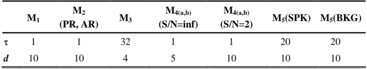
=0 for f < ). Signals were not prefiltered before 0 application of the Hilbert transform. For the wavelet transform, we implemented a continuous wavelet method (so-called ‘Morlet wavelet’). Measures (WR, WE) built from the wavelet transform were obtained from averaging over frequency sub-bands. For the generalized synchronization methods (S, N, H, SL), state space reconstruction parameters details (i.e., time lag τ and embedding dimension d) for all models are summarized in Table IV. In addition, for these methods,

the Theiler correction was chosen equal to time lag τ to prevent the information redundancy in used data.

APPENDIX C: CONFIDENCE INTERVALS ON MEASURED VALUES

Given c_i value, we assume that the estimations T_ki =Rˆ_L

(

x yi_k, _ki

)

,k =1,..,N are random variables

that obey the same probability distribution as the random variable 2 2 2

1 i i K i k i a

∑

u = a χ_K2 where

is a scaling parameter and where the are mutually independent and identically

distributed (index i stipulate the dependence on parameter ) Gaussian random variables, with zero

i

a uk Ki

i

c

mean and unit variance. The 2

i

K

χ term corresponds to a χ law with 2

degrees of freedom. Indeed, the

i

K

2

χ approximation was found to approximate histograms computed from simulated better than Gaussian distribution.

i k

T

Classical derivations from Gaussian moments properties give the following relationship:

( )

i 2 k i i E T = K a and

( )

4 2 i k

V A R T = K a_{i i} . Hence, the two parameters 2 and

i

a K_i can be

estimated by application of the moments estimation method which leads to formulas ˆ2 ˆ 2 i i i S a θ = and 2 ˆ ˆ 2 i i i K S θ = where 2 1 1 _ˆ ( 1 N i i k k S T N = θi) =

−

∑

− is the unbiased estimated variance of and

i k T 1 1 ˆ N i i k k T N θ = =

∑

its estimated mean.

Considering furthermore the random variables 2

1 1 _ˆ ( ) 1 N i i k i k S T N = θ = − −

∑

, 1 0 1 M i i S S M − = =

∑

, and 0 2 0 1 1 ( ) N k k MQ T N =

=

∑

, the problem is to quantify roughly their statistical dispersions. Although the

pdf of i are not Gaussian, those of

k

T θ , , and ˆi Si MQi can reasonably be modeled as Gaussian

(central limit effect). Consequently, approximations of corresponding standard deviations allow characterization of dispersions. • Variance of ˆ i θ 1 1 ˆ ( ) ( ) N i i i k k S VAR VAR T N N θ = =

∑

• Variances of S_i and S 2 2 2 1 2 1 1 _ˆ 1 ( ) ( ( ) ) ( ( ) ) ( 1) ( 1) N _i N _i i k k i k V A R S V A R T V A R T N = θ N = = − −

∑

−

∑

k 1 1 2 0 0 1 1 ( ) ( M _i) M ( _i) i i V A R S V A R S V A R S M M − − = = =

∑

=

∑

0 2 0 2 0 _{1 1} 1 1 ( ) ( N ( _k ) ) N ( ( _k ) ) k k V A R M Q V A R T V A R T N = N = =

∑

=

∑

Finally, the variance VAR T(( _ki) )2 =E T(( _ki) )4 −( ((E T_ki) ))2 2 is computed as follows.

)

Let μm' =E T( m and be moments of order m in the case where the mean of

random variable T is zero and none zero, respectively.

(( ( )) )m

m E T E T

μ = −

As T_ki is assumed to be a χ random variable, we can write (Stuart et al. [41]) that _K2 μ₂ =2K_i,

3 8Ki

μ = , and μ₄ =12K K_i( _i+4). From formulas (Stuart et al. [41], page 542) μ₂' =μ2+μ₁' 2,

' ' ' 2 ' 4

4 4 4 3 1 6 2 1 1

μ =μ + μ μ + μ μ +μ , we get the results:

' 2 2 2Ki Ki , μ = + ' 2 4 48 i 44 i 12 i 3 4 i K K K μ = + + + K 3 i ) which lead to 2 ' ' 2 2 4 2 ( ) 48 _i 40 _i 16 VAR T =μ −μ = K + K + K and finally to 2 8 2 3 2 4 _{ˆ ˆ}2 _ˆ3 ˆ (( _ki) ) (48 _i 40 _i 16 _i) ( ) (48 40 _i 16 _i VAR T =a K + K + K a K+ K + K REFERENCES

[1] J. S. Barlow and M. A. Brazier, "A note on a correlator for electroencephalographic work,"

Electroencephalogr Clin Neurophysiol Suppl, vol. 6, pp. 321-5, 1954.

[2] M. A. Brazier, "Studies of the EEG activity of limbic structures in man,"

Electroencephalogr Clin Neurophysiol, vol. 25, pp. 309-18, 1968.

[3] G. Pfurtscheller and C. Andrew, "Event-Related changes of band power and coherence: methodology and interpretation," Journal Of Clinical Neurophysiology: Official Publication Of The American Electroencephalographic Society, vol. 16, pp. 512-519, 1999.

[4] J. W. Cooley and J. W. Tukey, "An Algorithm for the Machine Calculation of Complex Fourier Series," Math. Comput., vol. 19, pp. 297-301, 1965.

[5] P. J. Franaszczuk and G. K. Bergey, "An autoregressive method for the measurement of synchronization of interictal and ictal EEG signals," Biol Cybern, vol. 81, pp. 3-9, 1999.

[6] S. Haykin, R. J. Racine, Y. Xu, and C. A. Chapman, "Monitoring neural oscillation and signal transmission between cortical regions using time-frequency analysis of electroencephalographic activity," Proceedings of IEEE, vol. 84, pp. 1295-1301, 1996.

[7] A. Pikovsky, M. Rosenblum, and J. Kurths, Synchronization : a universal concept in

nonlinear sciences. Cambridge: Cambridge University Press, 2001.

[8] N. J. Mars and F. H. Lopes da silva, "Propagation of seizure activity in kindled dogs,"

Electroencephalogr Clin Neurophysiol, vol. 56, pp. 194-209, 1983.

[9] J. P. Pijn and F. H. Lopes da silva, "Propagation of electrical activity: nonlinear associations and time delays between EEG signals," in Basic Mechanisms of the Eeg, Brain Dynamics, S. Zschocke and E. J. Speckmann, Eds. Boston: Birkhauser, pp. 41-61, 1993.

[10] F. Wendling, F. Bartolomei, J. J. Bellanger, and P. Chauvel, "Interpretation of interdependencies in epileptic signals using a macroscopic physiological model of the EEG," Clin Neurophysiol, vol. 112, pp. 1201-18, 2001.

[11] L. D. Iasemidis, "Epileptic seizure prediction and control," IEEE Trans Biomed Eng, vol.

50, pp. 549-58, 2003.

[12] K. Lehnertz, "Non-linear time series analysis of intracranial EEG recordings in patients with epilepsy--an overview," Int J Psychophysiol, vol. 34, pp. 45-52, 1999.

[13] M. Rosenblum, A. Pikovsky, and J. Kurths, "Synchronization approach to analysis of biological signals," Fluctuation Noise Lett., vol. 4, pp. L53-L62, 2004.

[14] J. Bhattacharya, "Reduced degree of long-range phase synchrony in pathological human brain.," Acta Neurobiol. Exp., vol. 61, pp. 309-318, 2001.

[15] J. Arnhold, P. Grassberger, K. Lehnertz, and C. E. Elger, "A robust method for detecting interdependences: application to intracranially recorded EEG," Physica D: Nonlinear Phenomena, vol. 134, pp. 419-430, 1999.

[16] C. J. Stam and B. W. van Dijk, "Synchronization likelihood: an unbiased measure of generalized synchronization in multivariate data sets," Physica D: Nonlinear Phenomena,

vol. 163, pp. 236-251, 2002.

[17] R. Quian Quiroga, A. Kraskov, T. Kreuz, and P. Grassberger, "Performance of different synchronization measures in real data: A case study on electroencephalographic signals,"

Physical Review E, vol. 65, 041903, 2002.

[18] O. David, D. Cosmelli, and K. J. Friston, "Evaluation of different measures of functional connectivity using a neural mass model," NeuroImage, vol. 21, pp. 659-673, 2004.

[19] F. Mormann, T. Kreuz, C. Rieke, R. G. Andrzejak, A. Kraskov, P. David, C. E. Elger, and K. Lehnertz, "On the predictability of epileptic seizures," Clinical Neurophysiology, vol.

116, pp. 569-587, 2005.

[20] E. Pereda, D. M. DelaCruz, L. DeVera, and J. J. Gonzalez, "Comparing Generalized and Phase Synchronization in Cardiovascular and Cardiorespiratory Signals," Biomedical Engineering, IEEE Transactions on, vol. 52, pp. 578-583, 2005.

[21] K. Ansari-Asl, J.-J. Bellanger, F. Bartolomei, F. Wendling, and L. Senhadji, "Time-Frequency Characterization of Interdependencies in Nonstationary Signals: Application to Epileptic EEG," Biomedical Engineering, IEEE Transactions on, vol. 52, pp. 1218-1226,

2005.

[22] A. S. Pikovsky, M. Rosenblum, and J. Kurths, "Synchronization in a population of globally coupled chaotic oscillators," Europhys. Lett., vol. 34, pp. 165-170, 1996.

[23] J. Bhattacharya, E. Pereda, and H. Petsche, "Effective detection of coupling in short and noisy bivariate data," Systems, Man and Cybernetics, Part B, IEEE Transactions on, vol. 33,

pp. 85-95, 2003.

[24] O. E. Rossler, "An equation for continuous chaos," Physics Letters A, vol. 57, pp. 397-398,

1976.

[25] M. Hénon, "A two-dimensional mapping with a strange attractor.," Communications in Mathematical Physics, vol. 50, pp. 69-77, 1976.

[26] F. Wendling, J. J. Bellanger, F. Bartolomei, and P. Chauvel, "Relevance of nonlinear lumped-parameter models in the analysis of depth-EEG epileptic signals," Biol Cybern, vol.

83, pp. 367-78, 2000.

[27] K. Ansari-Asl, F. Wendling, J. J. Bellanger, and L. Senhadji, "Comparison of two estimators of time-frequency interdependencies between nonstationary signals: application to epileptic EEG," 26th Annual International Conference of the Engineering in Medicine and Biology Society, San Francisco, Vol. 1, pp. 263, 2004.

[28] J. S. Bendat and A. G. Piersol, Random data : analysis and measurement procedures, 3rd

ed. New York: Wiley, 2000.

[29] F. Lopes da Silva, J. P. Pijn, and P. Boeijinga, "Interdependence of EEG signals: linear vs. nonlinear associations and the significance of time delays and phase shifts," Brain Topogr,

vol. 2, pp. 9-18, 1989.

[30] F. Wendling, F. Bartolomei, J. J. Bellanger, and P. Chauvel, "Interpretation of interdependencies in epileptic signals using a macroscopic physiological model of the EEG," Clinical Neurophysiology, vol. 112, pp. 1201-1218, 2001.

[31] J. P. Pijn, "Quantitative evaluation of EEG signals in epilepsy, nonlinear associations, time delays and nonlinear dynamics." Amsterdam: University of Amsterdam, 1990.

[32] M. Le Van Quyen, J. Foucher, J.-P. Lachaux, E. Rodriguez, A. Lutz, J. Martinerie, and F. J. Varela, "Comparison of Hilbert transform and wavelet methods for the analysis of neuronal synchrony," Journal of Neuroscience Methods, vol. 111, pp. 83-98, 2001.

[33] P. Tass, M. G. Rosenblum, J. Weule, J. Kurths, A. Pikovsky, J. Volkmann, A. Schnitzler, and H.-J. Freund, "Detection of n:m phase locking from noisy data: application to magnetoencephalography," Physical Review Letters, vol. 81, pp. 3291-3294, 1998.

[34] F. Mormann, K. Lehnertz, P. David, and C. E. Elger, "Mean phase coherence as a measure for phase synchronization and its application to the EEG of epilepsy patients," Physica D: Nonlinear Phenomena, vol. 144, pp. 358-369, 2000.

[35] F. Takens, "Lecture Nontes in Mathematics," Springer, vol. 898, pp. 366, 1981.

[36] A. M. Fraser and H. L. Swinney, "Independent coordinates for strange attractors from mutual information," Physical Review. A, vol. 33, pp. 1134-1140, 1986.

[37] L. Cao, "Practical method for determining the minimum embedding dimension of a scalar time series," Physica D: Nonlinear Phenomena, vol. 110, pp. 43-50, 1997.

[38] G. Osipov, A. Pikovsky, M. Rosenblum, and J. Kurths, "Phase synchronization effects in a lattice of nonidentical Rössler oscillators," Phys. Rev. E, vol. 55, pp. 2353-2361, 1997.

[39] S. J. Schiff, P. So, T. Chang, R. E. Burke, and T. Sauer, "Detecting dynamical interdependence and generalized synchrony through mutual prediction in a neural ensemble," Physical Review. E. Statistical Physics, Plasmas, Fluids, and Related Interdisciplinary Topics, vol. 54, pp. 6708-6724, 1996.

[40] R. Quian Quiroga, J. Arnhold, and P. Grassberger, "Learning driver-response relationships from synchronization patterns," Phys. Rev. E, vol. 61, 2000.

[41] M. G. Kendall, A. Stuart, J. K. Ord, S. F. Arnold, and A. O'Hagan, Kendall's advanced theory of statistics, 6th ed. London, New York: Edward Arnold; Halsted Press, 1994.

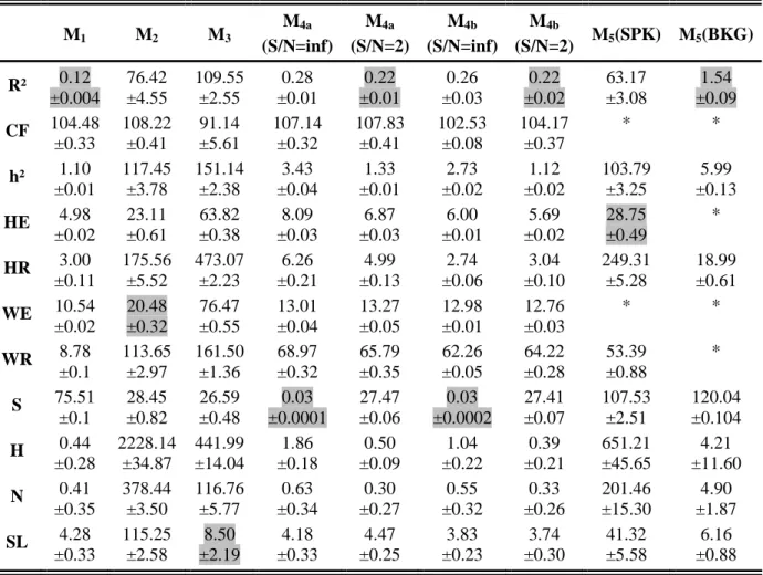
TABLE I. MSE Values and standard deviations (see Appendix C for computation) for studied methods and models. "*" denotes methods that are nearly insensitive to changes in the coupling degree and for which this criterion is not applicable.

M1 M2 M3 M4a (S/N=inf) M4a (S/N=2) M4b (S/N=inf) M4b (S/N=2) M5(SPK) M5(BKG) R² 0.12 ±0.004 76.42 ±4.55 109.55 ±2.55 0.28 ±0.01 0.22 ±0.01 0.26 ±0.03 0.22 ±0.02 63.17 ±3.08 1.54 ±0.09 CF 104.48 ±0.33 108.22 ±0.41 91.14 ±5.61 107.14 ±0.32 107.83 ±0.41 102.53 ±0.08 104.17 ±0.37 * * h² 1.10 ±0.01 117.45 ±3.78 151.14 ±2.38 3.43 ±0.04 1.33 ±0.01 2.73 ±0.02 1.12 ±0.02 103.79 ±3.25 5.99 ±0.13 HE 4.98 ±0.02 23.11 ±0.61 63.82 ±0.38 8.09 ±0.03 6.87 ±0.03 6.00 ±0.01 5.69 ±0.02 28.75 ±0.49 * HR 3.00 ±0.11 175.56 ±5.52 473.07 ±2.23 6.26 ±0.21 4.99 ±0.13 2.74 ±0.06 3.04 ±0.10 249.31 ±5.28 18.99 ±0.61 WE 10.54 ±0.02 20.48 ±0.32 76.47 ±0.55 13.01 ±0.04 13.27 ±0.05 12.98 ±0.01 12.76 ±0.03 * * WR 8.78 ±0.1 113.65 ±2.97 161.50 ±1.36 68.97 ±0.32 65.79 ±0.35 62.26 ±0.05 64.22 ±0.28 53.39 ±0.88 * S 75.51 ±0.1 28.45 ±0.82 26.59 ±0.48 0.03 ±0.0001 27.47 ±0.06 0.03 ±0.0002 27.41 ±0.07 107.53 ±2.51 120.04 ±0.104 H 0.44 ±0.28 2228.14 ±34.87 441.99 ±14.04 1.86 ±0.18 0.50 ±0.09 1.04 ±0.22 0.39 ±0.21 651.21 ±45.65 4.21 ±11.60 N 0.41 ±0.35 378.44 ±3.50 116.76 ±5.77 0.63 ±0.34 0.30 ±0.27 0.55 ±0.32 0.33 ±0.26 201.46 ±15.30 4.90 ±1.87 SL 4.28 ±0.33 115.25 ±2.58 8.50 ±2.19 4.18 ±0.33 4.47 ±0.25 3.83 ±0.23 3.74 ±0.30 41.32 ±5.58 6.16 ±0.88

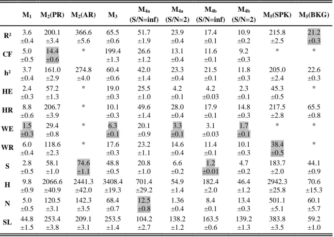
TABLE II. MV Values and standard deviations. "*" denotes methods that are nearly insensitive to changes in the coupling degree and for which this criterion is not applicable.

M1 M2(PR) M2(AR) M3 M4a (S/N=inf) M4a (S/N=2) M4b (S/N=inf) M4b (S/N=2) M5(SPK) M5(BKG) R² 3.6 ±0.4 200.1 ±3.4 366.6 ±5.6 65.5 ±0.6 51.7 ±1.9 23.9 ±0.4 17.4 ±0.1 10.9 ±0.2 215.8 ±2.5 21.2 ±0.3 CF 5.0 ±0.5 14.4 ±0.6 * 199.4 ±1.3 26.6 ±1.2 13.1 ±0.4 11.6 ±0.1 9.2 ±0.3 * * h² 3.7 ±0.4 161.0 ±2.9 274.8 ±4.0 60.4 ±0.6 42.0 ±1.4 23.3 ±0.4 21.5 ±0.1 11.8 ±0.3 205.0 ±2.4 22.6 ±0.3 HE 2.4 ±0.3 57.2 ±1.3 * 19.0 ±0.3 25.5 ±1.0 4.2 ±0.1 4.2 ±0.03 2.3 ±0.1 45.3 ±0.5 * HR 8.8 ±0.6 206.7 ±3.9 * 10.1 ±0.3 49.6 ±1.4 28.0 ±0.4 17.9 ±0.1 14.8 ±0.3 217.5 ±2.8 65.5 ±0.8 WE 1.5 ±0.3 29.4 ±0.8 * 6.3 ±0.1 20.1 ±0.9 3.3 ±0.1 3.1 ±0.03 1.7 ±0.1 * * WR 6.0 ±0.4 118.6 ±2.3 * 17.6 ±0.3 23.2 ±1.1 14.6 ±0.4 11.4 ±0.1 10.1 ±0.3 38.4 ±0.5 * S 2.8 ±0.5 58.1 ±1.0 74.6 ±1.1 48.8 ±0.5 20.8 ±1.0 6.6 ±0.2 1.2 ±0.01 4.7 ±0.2 183.7 ±2.0 44.1 ±0.9 H 9.8 ±0.9 2066.6 ±40.9 2441.3 ±42.0 3408.4 ±19.3 701.4 ±29.2 54.9 ±1.4 182.4 ±2.0 46.4 ±1.2 2942.3 ±25.8 70.6 ±15.3 N 5.0 ±0.5 120.5 ±3.1 142.3 ±3.5 68.4 ±0.7 12.5 ±0.8 1.36 ±0.4 8.4 ±0.1 13.4 ±0.3 501.1 ±5.1 60.1 ±5.7 SL 44.8 ±1.5 253.4 ±3.8 209.1 ±3.1 253.5 ±1.4 104.2 ±2.7 138.2 ±1.2 163.5 ±0.6 139.2 ±1.3 383.8 ±3.5 59.2 ±1.0

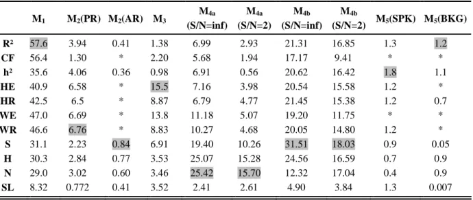
TABLE III. MRLS Values. "*" denotes methods that are nearly insensitive to changes in the coupling degree and for which this criterion is not applicable.

M1 M2(PR) M2(AR) M3 M4a (S/N=inf) M4a (S/N=2) M4b (S/N=inf) M4b (S/N=2) M5(SPK) M5(BKG) R² 57.6 3.94 0.41 1.38 6.99 2.93 21.31 16.85 1.3 1.2 CF 56.4 1.30 * 2.20 5.68 1.94 17.17 9.41 * * h² 35.6 4.06 0.36 0.98 6.91 0.56 20.62 16.42 1.8 1.1 HE 40.9 6.58 * 15.5 7.16 3.98 20.54 15.58 1.2 * HR 42.5 6.5 * 8.87 6.79 4.77 21.45 15.38 1.2 0.7 WE 47.0 6.69 * 13.8 11.18 5.07 19.20 11.75 * * WR 46.6 6.76 * 8.83 10.27 4.68 20.05 14.80 1.2 * S 31.1 2.23 0.84 6.91 19.40 10.26 31.51 18.03 0.9 0.05 H 30.3 2.84 0.77 3.53 25.07 15.28 24.56 16.59 0.7 0.9 N 29.0 3.02 0.60 3.46 25.42 15.70 12.32 17.04 0.4 0.9 SL 8.32 0.772 0.41 3.52 2.41 2.61 4.90 3.84 1.3 0.007

TABLE IV. State space reconstruction parameters used in computing the interdependencies by generalized synchronization methods

M1 M2 (PR, AR) M3 M4(a,b) (S/N=inf) M4(a,b) (S/N=2) M5(SPK) M5(BKG) τ 1 1 32 1 1 20 20 d 10 10 4 5 10 10 10