Entropy-satisfying scheme for a hierarchy of dispersive reduced models of free surface flow

HAL Id: hal-01242128

https://hal.inria.fr/hal-01242128v4

Submitted on 25 Jul 2019

HAL is a multi-disciplinary open access

archive for the deposit and dissemination of

sci-entific research documents, whether they are

pub-lished or not. The documents may come from

teaching and research institutions in France or

abroad, or from public or private research centers.

L’archive ouverte pluridisciplinaire HAL, est

destinée au dépôt et à la diffusion de documents

scientifiques de niveau recherche, publiés ou non,

émanant des établissements d’enseignement et de

recherche français ou étrangers, des laboratoires

publics ou privés.

reduced models of free surface flow

Martin Parisot

To cite this version:

Martin Parisot. Entropy-satisfying scheme for a hierarchy of dispersive reduced models of free surface

flow. International Journal for Numerical Methods in Fluids, Wiley, 2019, �10.1002/fld.4766�.

�hal-01242128v4�

dispersive reduced models of free surface flow

Martin Parisot

1

_{INRIA, CNRS, Sorbonne Université, Université Paris-Diderot SPC,}

Laboratoire Jacques-Louis Lions, project-team ANGE, F-75012 Paris,

France

June 24, 2019

Abstract

This work is devoted to the numerical resolution in the multidimensional framework of a hierarchy of reduced models of the water wave equations, such as the Serre-Green-Naghdi model. A particular attention is paid to the dissi-pation of mechanical energy at the discrete level, that act as a stability argu-ment of the scheme, even with source terms such space and time variation of the bathymetry. In addition, the analysis leads to a natural way to deal with dry areas without leakage of energy. To illustrate the accuracy and the robustness of the strategy, several numerical experiments are carried out. In particular, the strategy is capable of treating dry areas without special treatment.

1 Introduction

The propagation of surface waves is an essential issue for many applications such as port planning, tsunami propagation or marine energies. The dynamics of an in-compressible, homogeneous and inviscid fluid is governed by the monovalued free surface Euler model (E), also known as water wave equations. Unfortunately, (E) is too complex to be simulated at the scale of applications and some processes such as the wet/dry front or the breaking wave can be numerically unstable. For geophysi-cal applications, reduced models are widely used because they are easier and faster to solve numerically. The non-linear Shallow Water model (SW) is the simplest and most commonly used model nowadays. However, it is well known that (SW) is not a satisfactory model for wave propagation since dispersive effects are neglected. More precisely, the main assumptions for deriving (SW) from (E) are the so-called hydro-static pressure in the fluid Hp_{y p}) and the homogeneity of the horizontal velocity in

*_{martin.parisot@inria.fr}

the water column H_{y p}u ). These assumptions are described in more detail in §2.2. This work is devoted to the numerical resolution of the models that bypasse

Hy pp ), i.e. takes hydrodynamic pressure into account. In the past, some reduced

models have been derived from (E) to circumvent this assumption. The Serre-Green-Naghdi model (G N), see [22,32,35] is probably the most famous. Several simplified models of it are proposed in the literature and in the following we also consider the non-hydrostatic model (N H) [6] since it is easily classifiable in a hierarchy explained in §2.2. All these models have the particularity of being dispersive, even without source term, and we call them dispersive models in the following. Several works in the literature deal with the numerical resolution of these models. In [4,9,10], a nu-merical scheme is proposed based on a compact form of equations, i.e. where the only unknowns are the water depth and the horizontal velocity, using a splitting be-tween the shallow water equations (SW) and the dispersive part of the equations. Despite the splitting strategy, third order derivatives still required to be discretized. In [1], the authors propose a developed form of (N H), where the vertical-averaged vertical velocity is introduced. This new unknown added an equation to the hy-perbolic step and limited the dispersive step to a second-order elliptical pressure-based equation. In the current work, the elliptical equation is solved by a velocity-based scheme because it seems more relevant to deal with dry areas. Other strate-gies based on a new set of variables was proposed in the literature. For example in [27] Lagrangian variables are used. In [16], a relaxation of the constrains are used to obtained a hyperbolic system. However, the limit of the relaxation parameters to obtain the original Green-Naghdi model is not clear in the numerical framework. In addition, the entropic stability is not establish for these numerical scheme.

All the dispersive models satisfy the conservation of the mechanical energy. This property is fundamental from the point of view of mathematics because it is an ar-gument of stability for long time solution and for applications, particularly in renew-able energies.

The main novelty of the paper lies in the proof of entropy stability at the discrete level. Other models are studied in the literature to simulate two-phase flows, for example [18] and entropy-satisfying numerical scheme was proposed in such cases [11]. These models are generally hyperbolic and the numerical strategy for hyper-bolic models are well-understand nowadays [5,7]. In addition, level set strategy can also be used in this context [36]. However, these models also account the mass con-servation of air and are not well adapted to the case of geophysical flows. In the case of vertical-integrated models, some works propose stability property or even convergence results for the dispersive Korteweg-de Vries equation, i.e. for a scalaire dispersive equation in 1D [12,15]. To our knowledge, this work is the first numerical scheme for dispersive systems in multi-dimensional framework where the dissipa-tion of numerical mechanical energy is proven.

This document is organized as follows. First, the free surface Euler model (E) is briefly presented in §2as well as the hierarchy of reduced models. Then, §3is devoted to the description of the numerical resolution within the multidimensional

framework of each model in the hierarchy. The numerical scheme is built step by step with the complexity of the models. In §3.4, a simple treatment of the bound-ary conditions is presented. Eventually, several numerical illustrations in a one-dimensional frame are presented in §4which validate the accuracy and robustness of the method.

2 The hierarchy of free surface flow models

2.1 Incompressible free surface Euler equations (

E

)

We consider an incompressible, homogeneous, inviscid free surface flow over a non-flat bathymetry subjected to the force of gravity. The frame (t , x, z) is such that t ≥ 0 is the time, x ∈ Ω ⊂ Rd is the coordinate of the horizontal plane with d ∈ {1,2}, and

z ∈ R is the vertical coordinate oriented in such a way that z increases upwards.

The flow is supposed to satisfy the free surface incompressible Euler equations with a hypothesis of free surface monovalued. More precisely, the fluid is assumed to be contain between a given lower surface z = B (t, x) design as the bottom and an unknown free surface level z = η(t, x) ≥ B (t, x), and satisfies for any B < z ≤ η (E )    ∇ · u + ∂zw = 0 ∂tu + (u · ∇)u + w∂zu = −∇p ∂tw + (u · ∇) w + w∂zw = −∂zp − g

with ∇ and ∇· are respectively the gradient and the divergence according the x-variable, the horizontal velocity u (t , x, z) ∈ Rd, the vertical velocity w (t , x, z) ∈ R, the pressure in the fluid p (t , x, z) ∈ R and the gravity acceleration g ∈ R. At bottom, the condition of non-penetration is taken into account, i.e.

∂tB + u|z=B· ∇B = w|z=B

and at free surface, the pressure is given by p¡t, x,η(t,x)¢ = P (t,x) and the

kine-matic condition is taken into account, i. e.

∂tη + u|z=η· ∇η = w|z=η.

The system of equation must be completed with an initial conditionη(0,x) = η0(x),

u (0, x, z) = u0(x, z) and w (0, x, z) = w0(x, z) which has to satisfied the compatibility conditions with the divergence free condition and the boundary condition at bot-tom, i.e. (1) _{∇ · u}0_{+ ∂}zw0= 0 and ∂tB|t =0+ u 0 |z=B· ∇B = w 0 |z=B.

For readability, we introduce the homogeneous potential

φ(t,x) = gB (t,x) + P (t,x)

and the hydrodynamic pressure, also called non-hydrostatic pressure, defined by

q (t , x, z) = p (t, x, z) − P (t, x) − g¡

η(t,x) − z¢.

face f N k f k Cell k hn_k, un_k wn_k,σn_k q_B,kn , qn_k Cell k_f x y x z η B h u w σ qB q

Figure 1: Illustration of the notations. (left) Interpretation of the unknowns in the vertical plan. (right) Finit volume discretization in the horizontal plan.

Proposition 1. Assumingη0(x) − B (0, x) ≥ 0,

then the solution of (E) satisfies

1.i) the water depth positivity, i.e.η(t,x) − B (t,x) ≥ 0.

1.ii) the mechanical energy conservation for a sufficiently smooth solution, i.e. ∂t ¡ E ¡η − B¢ + Ku + Kw¢ + ∇ · ¡Gη+ Gu+ Gw+ Gq¢ = ¡ η − B¢∂tφ + q|z=B∂tB

with the potential energy

(2) E (h) = h µ φ + gh 2 ¶ ,

the kinetic energy_Kψ_{= K}¡

η,ψ¢ with K ¡η,ψ¢ =Zη B 1 2 ¯ ¯ψ¯¯ 2 dz,

and the flux are defined byGη= G¡

η,u,P + gη¢, Gu_{= G}¡ η,u,1 2kuk2¢,Gw = G ¡η,u,1 2|w| 2_{¢ andG}q = G¡η,u,q¢ with G ¡η,u,ψ¢ =Z η B ψu dz.

2.2 Brief description of the vertical-integrated models

In the current section, we present the hierarchy of vertical-integrated models of (E) that are considered in the sequel.

2.2.1 Shallow water model (SW)

First of all, we present (SW) [13] where the hydrodynamic pressure is neglected. The unknowns of (SW) are the water depth hSW_{(t , x) ∈ R}

horizontal velocity uSW

(t , x) ∈ Rd, see Figure1. More precisely, the unknowns of (E) are approximated by

η ≈ B + hSW_,

u ≈ uSW_,

w ≈ 0 and q ≈ 0.

(SW) can be obtained from (E) mainly assuming that:

Hy pp ) the pressure is hydrostatic, i.e. p (t , x, z) ≈ P (t, x) + g

¡

η(t,x) − z¢.

H_{y p}u ) the horizontal velocity is close to its vertical-average, i.e. u (t , x, z) ≈ u (t, x). A fine derivation from the Navier-Stokes equations is carried out in [19]. It is shown that (SW) is an approximation of a sufficiently smooth solution of Navier-Stokes equations in O (_{ε) where ε is the ratio of the vertical characteristic length to the} hor-izontal characteristic length. A higher order approximation can be derived, but it introduces dissipative terms.

2.2.2 Non-hydrostatic model (N H)

In the simplest dispersive model subsequently considered (N H) [6], the vertical ve-locity is approached by its vertical-averaged and leads to a linear approximation of hydrodynamic pressure. The unknowns of (N H) are the water depth hNH_{(t , x) ∈ R}

+,

the vertical-averaged horizontal velocity uNH

(t , x) ∈ Rd, the vertical-averaged verti-cal velocity wNH(t , x) ∈ R and the hydrodynamic pressure at bottom qNH

B (t , x) ∈ R,

see Figure1. More precisely, the unknowns¡u, w, q¢ of (E) are approximated in the vertical direction inP0× P0× P1such that

η ≈ B + hNH_, u ≈ uNH_, w ≈ wNH _and q ≈B + h − z h q NH B .

A fine derivation of (N H) from (E) is realized in [6].

2.2.3 Serre-Green-Naghdi model (G N)

To satisfy the divergence free condition, the vertical velocity approximation must be of one order higher than the horizontal velocity. In the simple case, the hori-zontal velocity is approached in the vertical direction by means of a constant func-tion, then the vertical velocity by means of a linear function and the hydrodynamic pressure by means of a quadratic function. It yields to (G N) [22,32,35]. The un-knowns of (G N) are the water depth hGN_{(t , x) ∈ R}

+, the vertical-averaged horizontal

velocity uGN

(t , x) ∈ Rd, the vertical-averaged vertical velocity wGN

(t , x) ∈ R, the ori-ented standard deviation of the vertical velocityσGN_{(t , x) ∈ R, the hydrodynamic}

pressure at bottom qGN

B (t , x) ∈ R and the vertical-averaged hydrodynamic pressure

qGN(t , x) ∈ R, see Figure1. More precisely, the unknowns¡u, w, q¢ of (E) are approx-imated in the vertical direction inP0× P1× P2such that

η ≈ B + hGN_, u ≈ uGN_, w ≈ wGN + 2p3z − B + h 2 h σ GN and q ≈B + h − z h q GN B + 3 (z − B)(B + h − z) h2 ¡2q GN − qBGN¢ .

Other reconstructions of (E) unknowns from that of the Serre-Green-Naghdi model can be done in particular to satisfy a curl free condition of the divergence free con-dition. A finer derivation of (G N) from (E) and a more detailed description is per-formed in [25]. It is shown that (G N) is an approximation of (E) in the order of O¡

ε2¢ and O (a) with a is the ratio between the characteristic wave amplitude and the char-acteristic water depth.

Other dispersive models, see [41], can be also considered and treated using a similar numerical strategy presented in the following. We limit the presentation to (N H) and (G N) for readability. In addition, the exponentsSW,NHandGNare re-moved when the model used is not confusing. More precisely, each of the following subsections is devoted to a single model and the unknowns refer to it.

For each model, an entropy-satisfying scheme based on Finite volume discretiza-tion is proposed. Let us introduce some of the notadiscretiza-tions used in the following.

A tesselationT of the horizontal domain Ω ⊂ Rdis considered, composed of N = Card (T) star-shaped control volumes, see Figure1. One denotes by k ∈ T a cell, Fk the set of its faces and |k| its surface area. Furthermore, for a face f , its length

is noted¯¯f ¯

¯and the neighbor of k through f is denoted by k

f such as k ∪ kf = f .

The unit normal to f outward to k is noted byN_kkf. To describe the schemes, the centered discrete operator ∇δ_k: (R)N→ Rdand ∇δ_k· :¡

Rd¢N

→ R are used respectively defined by (3) ∇δkψ = 1 |k| X f ∈Fk ψk_f+ ψk 2 N k_f k ¯ ¯f ¯ ¯ and ∇δk· ψ = 1 |k| X f ∈Fk ψk+ ψk_f 2 · N k_f k ¯ ¯f ¯ ¯.

These discrete operators are clearly consistent with ∇ and ∇· respectively and are second order. The time is discretized using an adaptive time step, i.e. tn+1= tn+δnt,

withδn_t satisfying a CFL condition described below. The discrete unknownsψn_k is the approximation of the mean value of the unknownsψ in the cell k at time tn. For readability, we introduce the discrete time derivative of a variableψ by

(4) ∂n+1_t ψ =ψ

n+1_{− ψ}n

δn t

3 Numerical schemes for the reduced models

3.1 Shallow water model (

SW

)

3.1.1 Governing equations of (SW) and main properties

Let us begin the description of the strategy with the well-known shallow water model (SW). It reads

(SW )

∂tUSW+ ∇ · FSW¡USW¢ = SSW¡USW¢ with USW=

µ h hu ¶ FSW_¡USW_{¢ =} µ _hu hu ⊗ u +g2h2Id ¶ and SSW_¡USW_{¢ =} µ 0 −h∇φ ¶ .

The initial condition of (SW) is given by h (0, x) = h0(x) and u (0, x) = u0(x). Let us recall the main physical properties of (SW).

Proposition 2. Assuming h0(x) ≥ 0,

then the solution of (SW) satisfies

2.i) the water depth positivity, i.e. h (t , x) ≥ 0. It is the counterpart of Proposition1.i).

2.ii) the mechanical energy conservation for a sufficiently smooth solution, i.e. ∂t ³ E + Ku´+ ∇ · ³ Gh+ Gu ´ = h∂tφ

with the potential energyE (h) defined by (2), the kinetic energy owing from

the horizontal velocityKu = K ¡h,u¢ and the fluxGh= G¡hu,φ + gh¢ and

Gu= G¡hu,K ¡1,u¢¢ with (5) K ¡h,ψ¢ =h 2 ° °ψ°° 2 and G ¡Q,ψ¢ = ψQ

More precisely, in case of non-smooth solution, the admissible solutions are de-fined such that the mechanical energy is decreasing, i.e.

∂t ³ E + Ku´+ ∇ · ³ Gh+ Gu ´ ≤ h∂tφ.

It is the counterpart of Proposition1.ii).

3.1.2 Entropy-satisfying numerical scheme of (SW)

In the past, several numerical strategies have been proposed that preserve main physical properties, in particular Proposition2. In the current work, we briefly recall one of them based on an explicit Finit Volume scheme. The scheme of (SW) can be formulate as (SWδ) U_kSW,n+1= U_kSW,n−δ n t |k| X f ∈Fk µ FSW,n f · N k_f k + S SW,n f ,k ¶ ¯ ¯f ¯ ¯

with U_kSW,n=¡hn k, h n ku n k ¢t

. Several strategies are described in the literature to com-pute the numerical fluxF_fSW,n =³F_f1,n,F2,n_f ´t and the source termS_{f ,k}SW,n of the shallow water model, see [5,20,28,38].

In the following, we ask (SWδ) to satisfy the following properties under a CFL condition like (6) λ µ U_kSW,n;U_kSW,n f ¶ δn t ≤ min ³ δk,δk_f ´

withδk the compactness of kf, i.e. δk = |k|₂ if d = 1 and δk = P |k|

f ∈Fk|f| if d = 2.

λ¡USW

L ;U

SW

R ¢ is an upper limit of the wave speed, depending on the numerical flux

FSW_{used, see [5].}

Hypothesis 1. Under the CFL condition (6) and for any positive initial data, i.e. h0_k≥ 0, the solution of (SWδ) satisfies

1.i) the water depth positivity, i.e. hn_k≥ 0.

It is the discrete counterpart of Proposition2.i).

1.ii) the discrete mechanical energy dissipation. More precisely, there exist two flux

Gh_δ¡USW L ;U SW R ¢ andG u δ¡ULSW,U SW

R ¢ respectively consistent withG h

andGugiven in (5) such that the discrete mechanical energy satisfies

∂n+1 t ³ Ek+ K u k ´ + 1 |k| X f ∈Fk ³ Gh,nf + G u,n f ´ · Nkkf ¯ ¯f ¯ ¯≤ hn k∂ n+1 t φk withE_kn _{= E}¡hn k¢,K u,n k =K ¡hnk,u n k¢,G h,n f =G h δ µ USW,n k ,U SW,n k_f ¶ andGu,n_{f =} Gu_δ µ U_kSW,n,U_kSW,n f ¶ .

It is the discrete counterpart of Proposition2.ii).

For homogeneous potential, i.e. ∇φ = 0, some numerical strategies ensure the entropy stability Hypothesis1.ii). This is the case, for example, of Godunov solver [21], of the kinetic solver [33] and of the Suliciu relaxation solver [37]. In the case of a source term, the numerical strategy only ensure a semi-discrete entropy stability, i.e. before discretization in time, see [5]. Some implicit or ImEx schemes ensure the entropy stability with the source term, see instead [31], and can also be used with the numerical strategy of the dispersive models presented in the following.

Note that the Hypothesis1is not an exhaustive list of properties that we can ask for (SW), for instead the conservation of the steady state. Even if the translation of these properties at the discrete level is an interesting and stimulating question, this is not the purpose of the current work.

3.2 Non-hydrostatic model (

N H

)

3.2.1 Governing equations of (N H) and main properties

Let us now focus on the second assumption Hy pp ). The simplest model in the

as follows (N H .a)      ∂th + ∇ ·¡hu ¢ = 0 ∂t¡hu¢ + ∇ · ³ hu ⊗ u +g 2h 2_I d ´ + h∇φ = −∇ ³ hqB 2 ´ − qB∇B ∂t¡hw¢ + ∇ · ¡hw u¢ = qB

with the hydrodynamic pressure qBrelated to the constraint

(N H .b) w = ∂t µ B +h 2 ¶ + u · ∇ µ B +h 2 ¶ .

The initial condition h (0, x) = h0(x), u (0, x) = u0(x) and w (0, x) = w0(x) must sat-isfy the compatibility condition

(8) w0= ∂tB|t =0+ u 0 · ∇B −h 0 2 ∇ · u 0

which corresponds to the vertical-averaged of the compatibility condition (1). For more detail about (N H), we refer to [6]. Let us first recall the main physical proper-ties of (N H).

Proposition 3. Assuming that h0_{(x) ≥ 0,}

then the solution of (N H) satisfies

3.i) the water depth positivity, i.e. h (t , x) ≥ 0. It is the counterpart of Proposition1.i).

3.ii) the mechanical energy conservation for a sufficiently smooth solution, i.e. ∂t ³ E + Ku+ Kw ´ + ∇ · ³ Gh+ Gu+ Gw+ Gq NH´ = h∂tφ + qB∂tB

with the potential energy_{E (h) defined by (}2), the kinetic energiesKψ= K¡h,ψ¢, and the fluxGh_{= G}¡hu,φ + gh¢, Gu= G¡hu,K ¡1,u¢¢, Gw= G¡hu,K ¡1,w¢¢,

and_Gq

NH

= G¡hu,qB

2¢ defined by (5).

It is the counterpart of Proposition1.ii).

3.2.2 Entropy-satisfying numerical scheme of (N H)

Now we focus on describing a numerical strategy for solving (N H). As in previous works [1,4,9,26], the numerical scheme is based on a splitting strategy between the advection step and the dispersion step. The splitting strategy is a well unknown solution to design numerical scheme for models where a part of the equation is hy-perbolic [24]. The advantage of this strategy is to use the classic scheme (SWδ) for the advection part. In particular, thanks to the formulation (N H), the advection (left-hand side) of the vertical velocity is solved by conventional passive transport scheme. This strategy has already been used in [1] and entropy-satisfying schemes to solve it can be used [5]. However, in the cited works, the dispersion step is solved

using a prediction-correction strategy based on an implicit system on the hydrody-namic pressure qB. Another strategy to solve the dispersive model is to write the

equation on horizontal velocity, see [4,9,26]. The advantage of this strategy is that dissipative forces such as friction or viscous terms can also be taken into account simultaneously with dispersion. Unfortunately, without the introduction of vertical velocity, this strategy reveals third order derivatives that are not easy to discretize. The scheme proposed in the current work attempts to address the benefits of both strategies. More precisely, the vertical velocity is introduced and advected during the hyperbolic step and the dispersion step is resolved using an elliptical equation on the horizontal velocity. Even if dissipative forces, friction and viscous terms, can be taken into account simultaneously with dispersion as in previous strategies based on horizontal velocity, we do not deal with these terms in this work for readability. We reformulated (N H) as (9) ∂tUNH+ ∇ · FNH¡UNH¢ = SNH¡UNH¢ + DNH with UNH =µU SW hw ¶ , FNH_¡UNH_{¢ =}µFSW¡USW ¢ hw u ¶ SNH_¡UNH_{¢ =}µSSW¡USW ¢ 0 ¶ and DNH =   0 −∇¡hqB 2¢ − qB∇B qB  .

Let’s now assume that the water depth, the horizontal velocity and vertical ve-locity at the time of iteration n are known, i.e. h_kn, un_kandwn_k, as for example at the initial condition. Then, the time step can be split into three steps, briefly described as follows:

1. The advection step (N Hδ.a), where the advection and the conservative forces are solved using (SWδ).

2. The dispersion step (N Hδ.b), where the dispersive operator, and eventually the dissipative forces, are solved using an implicit finite volume method.

Advection and conservative forces:

This step is based on (SWδ). More precisely, by neglecting the dispersal operator

DNH_{, the first two unknowns of U}NH _{are estimated using (SW}δ_{) while the third is}

simply advected to the flow as a passive pollutant, see [5]. This strategy was already used for dispersive model in [1]. We write

(N Hδ.a) U_kNH,n?= U_kNH,n−δ n t |k| X f ∈Fk µ FNH,n f · N k_f k + S NH,n f ,k ¶ ¯ ¯f ¯ ¯

with the state vector U_kNH,n=¡USW,n

k , h n kw n k ¢t

, the source termS_{f ,k}NH,n= ³

SSW,n

f ,k , 0

´t , the numerical flux

FNH,n f · N k_f k =    FSW,n f · N k_f k F_δup µ F1,n f · N k_f k , ³ wn_k, wn_k f ´¶   

with the up-wind scheme

(11) F_δup¡Q,¡ψL,ψR¢¢ = ψLQ+− ψRQ−

and the positive and negative part functions are defined byψ_{±= |}ψ|₂±ψ.

Dispersion and dissipative forces:

Now let us introduce the scheme of the dispersion step. Since the water depth is not affected by this step, we have defined hn+1_{k = h}n_k?. Then, wherever the water depth does not vanishes, the horizontal velocity is corrected by the following implicit linear scheme (N Hδ.b) αNH k un+1k + ∇δk ¡ µNH · un+1¢ − µkNH∇δk· un+1− ∇δk ³ κNH ∇δ· un+1 ´ = βNHk

with the discrete operators ∇δ_kand ∇δ_k· defined by (3) and the parameters

αNH k = h n? k ³ Id+ ∇δkBn+1⊗ ∇δkBn+1 ´ , µNH k = ¡hn? k ¢2 2 ∇ δ kBn+1, κ NH k = ¡hn? k ¢3 4 , and βNH k = h n? k u n? k + h n? k ¡w n? k − ∂n+1t Bk¢ ∇δkBn+1 +∇δk à ¡hn?¢2 2 ¡w n?_{− ∂}n+1 t B ¢ ! .

In the dry zone, the scheme leads to a trivial equation and the resulting linear system is not well-posed. To overcome this issue, in all dry cells, (N Hδ.b) is replaced by

un+1_{k = 0. The solution is obviously influenced by the choice of velocity in dry areas.}

However, this choice is motivated by the conservation of the mechanical energy at the dry front, see Proposition4. More precisely, thanks to this choice, the energy flux of the dispersive part vanishes on the dry front.

Finally, the vertical velocity is reconstructed using the following scheme (N Hδ.c) _wn+1 k = ∂n+1t Bk+ un+1k · ∇δkBn+1− hn+1 k 2 ∇ δ k· un+1

where the discrete time derivative is defined by (4) and the discrete operators are defined by (3).

Let’s explain how the scheme is obtained. (N Hδ.c) is obtained after a rewriting of (N H .b) using the mass conservation (first equation of (N H .a)) as

w = ∂tB + u · ∇B −

h

2∇ · u.

Even if other writings of the constraint can be considered, a discretization of this one ensures the entropy stability at the discret level, see Proposition4. (N Hδ.b) is obtained by considering the following discretization of the dispersive operator (13) U_kNH,n+1= U_kNH,n?+ δntD NH,n+1 k ¡q n+1 B ¢

with DNH,n k ¡qB¢ =    0 −∇δk ³ hnqB 2 ´ − qB,k∇δkB n qB,k   .

Together with (N Hδ.c), they form a (d + 2) × N linear system (without h). Fortu-nately, this system can be reduced by simple substitution and leads to the d × N linear system (N Hδ.b).

Proposition 4. Assuming Hypothesis1, h_k0≥ 0 and the CFL condition (6) holds. Then

the solution of (N Hδ) satisfies

4.i) the water depth positivity, i.e. hn_{k≥ 0.}

It is the discrete counterpart of Proposition3.i). 4.ii) the discrete mechanical energy dissipation, i.e.

∂n+1 t ³ Ek+ K u k+ K w k ´ + 1 |k| X f ∈Fk ³ Gh,nf + G u,n f + G w ,n f + G qNH_,n+1 f ´ · Nkkf ¯ ¯f ¯ ¯ ≤ hnk∂n+1t φk+ qB,kn+1∂n+1t Bk

with the energiesE_kn_{= E}¡hn k¢,K ψ,n k = K¡hnk,ψ n k¢ defined by (5), the fluxGh,n_{f = G}h_δ Ã µ _hn k hn_kun_k ¶ , Ã _hn k_f h_kn fu n k_f !! ,Gu,n_{f = G}u_δ Ã µ _hn k hn_kun_k ¶ , Ã _hn k_f h_kn fu n k_f !!

intro-duced in Hypothesis1.ii),Gw ,n_f = F_δup  F1,n f · N k_f k ,   ¡wn k ¢2 2 , µ wn_{k f} ¶2 2    defined by (11) andGq NH_,n f = G q δ         hn_k un_k qn B,k 2   ,      h_kn f un_k f qn B,k f 2           defined by Gq_δ     hL uL q_L  ,   hR uR q_R    = hLqL+ hRqR 2 uL+ uR 2 − hRqR− hLqL 2 uR− uL 2 .

It is the discrete counterpart of Proposition3.ii).

Proof. Proposition4.i)is an obvious consequence of Hypothesis1.i).

Let’s focus on mechanical energy conservation Proposition4.ii). Thanks to Hy-pothesis1.ii), we have

(14) E n? k + K u,n? k + δn t |k| X f ∈Fk ³ Gh,nf + G u,n f ´ · N_kkf¯¯f ¯ ¯ ≤ Ekn+ K u,n k + hkn ¡ φn+1 k − φ n k ¢

withE_kn?_{= E}¡hn? k ¢ andK ψ,n? k = K¡hkn?,ψ n? k ¢.

Similarly, a classical result of the Suliciu relaxation is the following entropy in-equality as long as the positivity is ensured, see [5, Chapter 2.7]

(15) Kkw ,n?+ δn t |k| X f ∈Fk Gw ,nf ¯ ¯f ¯ ¯≤ K w ,n k .

Now, we focus on the dispersion step (N Hδ.b)-(N Hδ.c). As explained above, the dispersion step (N Hδ.b) is equivalent to (13). By multiplying the second equation of (13) by un+1_k , it yields (16) Ku,n+1_k ≤Ku,nk ?− δnt à un+1_k · ∇δk à hn+1q n+1 B 2 ! + qn+1B,kun+1k · ∇δkBn+1 ! .

Thanks to the centered operator (3), the following relation holds

un+1_{k · ∇}δ_k à hn+1q n+1 B 2 ! = 1 |k| X f ∈Fk GqfNH,n+1· N k_f k ¯ ¯f ¯ ¯− q_B,kn+1 hn+1_k 2 ∇ δ k· un+1.

Then by multiplying the third equation of (13) by wn+1_k , it yieds

(17) _Kw ,n+1_{k ≤ K}w ,n_k ?_{+ δ}n

tqB,kn+1w n+1

k .

Summing the energy dissipations (16) and (17), it yields

(18) Ku,n+1k + K w ,n+1 k + δn t |k| X f ∈Fk GqfNH,n+1· N k_f k ¯ ¯f ¯ ¯≤ K u,n? k + K w ,n? k +δntqB,kn+1 à wn+1_k − un+1k · ∇δkBn+1+ hn+1_k 2 ∇ δ k· un+1 ! .

Finally, we conclude by using (N Hδ.c). At wet/dry fronts, the water level vanishes in a cell, for instance hR= 0. Then the energy flux is proportional to the velocity in

the dry cell, i.e.G_δq₌hLqL

2 uR. By setting uR= 0, the flux through the wet/dry fronts

vanishes.

Remark 1. The dissipative term such are friction and viscosity can easily be treated

si-multaneously with dispersion. More precisely, it only adds the corresponding reaction and diffusion terms in (N Hδ.b).

Remark 2. A drawback of (N Hδ.b) is its large stencil, i.e. the 5-point stencil in 1D.

Some may want to replace (N Hδ.b) with a more compact and simpler discrete

op-erator, see AppendixA. However, the entropy stability Proposition4.ii)is lost and in practice the numerical results are less accurate, see4.2.

Remark 3. Some people may rather like to solve the linear system by keeping one

of the other unknowns after substitution. For example, in [1], the dispersion step is solved by maintaining the hydrodynamic pressure qBas unknown to the linear

sys-tem. This choice is particularly attractive for multidimensional simulations, since u ∈ Rdwhereas qB∈ R. However, this formulation is less practical for imposing zero

velocity in dry areas. Moreover, it is not possible to treat friction and viscosity, if any, in the same step, contrary to the formulation (N Hδ.b).

Let us define the set of admissible solutions for (N H) (19) ANH_r ,n= ½ ¡u, w¢ ∈ ¡RN¢d +1 ¯_¯ ¯ ° ° ° °∂ n tB + uk· ∇δBn− hn 2 ∇ δ_{· u − w}°° ° ° δ≤ r ¾ . with k•kδis a discret norm on the tessellationT. In the following we use the L2-norm

° °φ°°_δ=

X

k∈T

|k|φ2k.

Proposition 5. The dispersion step (N Hδ.b) is a projection on the set of velocity

sat-isfying the constrain (N Hδ.c).

More precisely¡un+1_{, w}n+1_{¢ ∈ A}NH,n+1 0

and if¡un?_{, w}n?_{¢ ∈ A}NH,n+1

0 then¡un+1, wn+1¢ = ¡u

n?_{, w}n?_¢.

3.3 Serre-Green-Naghdi model (

G N

)

3.3.1 Governing equations of (G N) and main properties

As it was mentioned in [17], the non-hydrostatic model (N H) is not completely co-herent with (E). More precisely, the vectorial space of the approximation for u and

w , i.e. both inP0(z), is not coherent with the divergence free condition. To make

the approximation coherent with the divergence free condition when u is inP0(z),

w must be approximated inP1(z), see §2.2.3and [17] for more details. It is the case

for the Serre-Green-Naghdi model (G N), see [22,32,35].

To propose a scheme in the spirit of (N Hδ), (G N) is reformulated as follows

(G N .a)            ∂th + ∇ ·¡hu¢ = 0 ∂t¡hu ¢ + ∇ ·³hu ⊗ u +g 2h 2_I d ´ = −h∇φ − ∇¡hq¢ − qB∇B ∂t¡hw¢ + ∇ · ¡hw u¢ = qB ∂t(hσ) + ∇ · ¡hσ u¢ = p 3¡2q − qB ¢

with the hydrodynamic pressures q and qBrelated to constraints (N H .b) and

(G N .b) _{σ =}∂th + u · ∇h 2p3 .

The initial condition h (0, x) = h0(x), u (0, x) = u0(x), w (0, x) = w0(x) andσ(0,x) =

σ0_{(x) must satisfy the compatibility conditions (8) and}

(21) σ0= − h

0

2p3∇ · u

which corresponds to the vertical-averaged of the standard deviation of the compat-ibility condition (1). In [17] it is shown that (G N) is equivalent, at least for smooth solution, to the classical Peregrine formulation [32]. Let us first recall the main phys-ical properties of (G N).

Proposition 6. Assuming that h0(x) ≥ 0,

then the solution of (G N) satisfies

6.i) the water depth positivity, i.e. h (t , x) ≥ 0. It is the counterpart of Proposition1.i).

6.ii) the mechanical energy conservation for a sufficiently smooth solution, i.e. ∂t ³ E + Ku+ Kw+ Kσ ´ + ∇ · ³ Gh+ Gu+ Gw+ Gσ+ Gq GN´ = h∂tφ + qB∂tB

with the potential energyE (h) defined by (2), the kinetic energies Kψ_{= K}¡h,ψ¢ and the fluxGh= G¡hu,φ + gh¢, Gu= G¡hu,K ¡1,u¢¢, Gw= G¡hu,K ¡1,w¢¢, Gσ= G¡hu,K (1,σ)¢, Gq

GN

= G¡hu, q¢ defined by (5).

It is the counterpart of Proposition1.ii).

3.3.2 Entropy-satisfying numerical scheme of (G N)

Now we focus on describing a numerical strategy for solving (G N). Similarly to (N Hδ), (G N .a) is written as ∂tUGN+ ∇ · FGN¡UGN¢ = SGN¡UGN¢ + DGN with UGN =µU NH hσ ¶ , FGN_¡UGN_{¢ =}µFNH¡UNH ¢ hσ u ¶ SGN_¡UGN_{¢ =}µSNH¡UNH ¢ 0 ¶ and DGN =     0 −∇¡hq¢ − qB∇B qB p 3¡2q − qB ¢    

and the numerical strategy is based on the same two steps: advection and conser-vative forces, dispersion and dissipative forces.

Advection and conservative forces:

As done for (N Hδ.a), the advection and conservative forces are realized using the strategy (SWδ) with an up-wind scheme for the vertical velocities wn_k andσn_k. We write (G Nδ.a) U_kGN,n?= U_kGN,n−δ n t |k| X f ∈Fk µ FGN,n f · N k_f k + S GN,n f ,k ¶ ¯ ¯f ¯ ¯

with the state vectors U_kGN,n=¡UNH,n k , h n kσ n k ¢t

, the numerical flux

FGN,n f · N k_f k =    FNH,n f · N k_f k F_δup µ F1,n f · N k_f k , ³ σn k,σ n k_f ´¶   

with the upwind flux defined by (11) and the source termS_{f ,k}GN,n=³S_{f ,k}NH,n, 0´t.

Dispersion and dissipative forces:

As for (N Hδ), we set hn+1_k = hn_k?. In wet cell, i.e. hn+1_k > 0, we write (G Nδ.b) αGN k un+1k + ∇δk ¡ µGN · un+1¢ − µGN k ∇δk· un+1− ∇δk ³ κGN ∇δ· un+1´= βGN k

where the parameters read

αGN k = α NH k , µ GN k = µ NH k , κ GN k = 4 3κ NH k and β GN k = β NH k + 1 2p3∇ δ k ³ ¡hn?¢2 σn?´ .

and in dry cell we set un+1_{k = 0. Finally, the vertical velocity is reconstructed using} (N Hδ.c) and (G Nδ.c) σn+1_k = −h n+1 k 2p3∇ δ k· un+1.

The scheme (G Nδ.b) was obtained similarly to (N Hδ.b). More precisely, the dis-persive operator is discretized by

(23) U_kGN,n+1= U_kGN,n?+ δntD GN,n+1 k ³ qn+1, qn+1_B ´ with DGN,n k ¡q, qB¢ =      0 −∇δk¡h n_{q¢ − q} B,k∇δkB n qB,k p 3¡2q_{k− q}B,k ¢      .

Together with (G Nδ.c), it forms a (d + 3) × N linear system which can be reduced by simple substitution and leads to the d × N linear system (G Nδ.b).

Proposition 7. Assuming Hypothesis1, h_k0≥ 0 and the CFL condition (6) holds. Then

the solution of (G Nδ) satisfies

7.i) the water depth positivity, i.e. hn_k≥ 0.

7.ii) the discrete mechanical energy dissipation, i.e. ∂n+1 t ³ Ek+K u k+K w k +K σ k ´ + 1 |k| X f ∈Fk ³ Gh,nf + G u,n f + G w ,n f + G σ,n f + G qGN_,n+1 f ´ · Nkkf ¯ ¯f ¯ ¯ ≤ hkn∂n+1t φk+ qn+1B,k∂n+1t Bk

with the energiesE_kn_{= E}¡hn k¢,K ψ,n k = K¡hkn,ψ n k¢ defined by (5), the fluxGh,n_{f = G}h_δ Ã µ hn_k h_knun_k ¶ , Ã _hn k_f hn_k fu n k_f !! ,Gu,n_{f = G}u_δ Ã µ hn_k h_knun_k ¶ , Ã _hn k_f hn_k fu n k_f !!

intro-duced in Hypothesis1.ii),Gw ,n_f = F_δup  F1,n f · N k_f k ,   ¡wn k ¢2 2 , µ wn_{k f} ¶2 2    ,G σ,n f = F_δup  F 1,n f · N k_f k ,   ³ σn k ´2 2 , µ σn k f ¶2 2    defined by (11) andG qGN ,n f = G q δ       h_kn un_k qn_k  ,     h_kn f un_k f qn_k f        

is introduced in Proposition4.ii).

It is the discrete counterpart of Proposition6.ii).

Proof. Proposition7.i)is an obvious consequence of Hypothesis1.i).

Let us focus on the mechanical energy conservation Proposition7.ii). The proof is similar to the one of Proposition4.ii). Thanks to Hypothesis1.ii), we obtain (14). Using the properties of the up-wind scheme, we obtain (15) and

(24) Kσ,n?_k +δ n t |k| X f ∈Fk Gσ,nf ¯ ¯f ¯ ¯≤Kσ,n_k .

Now multiplying the second equation of (23) byun+1_k , it reads

(25) K u,n+1 k + δn t |k| X f ∈Fk GqfGN,n+1· N k_f k ¯ ¯f ¯ ¯≤K u,n? k +δnt ³ qn+1_k h_kn+1∇δk· un+1− qB,kn+1un+1k · ∇δkBn+1 ´ .

Then multiplying the third equation of (23) by wn+1_k , we get (17) and the fourth by

σn+1 k , we get

(26) Kσ,n+1_{k ≤}Kσ,n?_{k + δ}n_tp3³2qn+1_{k − qB,k}n+1´σn+1_k

Summing the energy dissipations (25), (17) and (26), it yields

(27) Ku,n+1k +K w ,n+1 k +K σ,n+1 k + 1 |k| X f ∈Fk GqfGN,n+1· N k_f k ¯ ¯f ¯ ¯ ≤ Ku,nk ?+ K w ,n? k + K σ,n? k + δnt2 p 3qn+1_k à σn+1 k + hn+1 k 2p3∇ δ k· un+1 ! +δntqB,kn+1 ³ wn+1_k −³un+1_k · ∇δkBn+1+ p 3σn+1_k ´´.

We conclude using (G Nδ.c) and summing with (14), (15) and (24).

Remark 4. Remarks1and2still holds for (G Nδ). Remark3still holds for (G Nδ) with

a slight revision of the conclusion. The system could be solved either with u ∈ Rd or with¡q, qB¢ ∈ R2as the main unknown. The first solution is clearly preferable while

d = 1 in addition to the fact that the dry areas are treated simply.

Let us define the set of admissible solutions for (G N)

(28) AGN,n r = ½ ¡u, w,σ¢ ∈ ANH,n r × RN ¯ ¯ ¯ ° ° ° °σ + hn 2p3∇ δ_{· u}°° ° ° δ≤ r ¾ .

Proposition 8. The second step of the scheme is actually a projection on the set of

velocity satisfying the constrain (N Hδ.c) and (G Nδ.c).

More precisely,¡un+1, wn+1,σn+1¢ ∈ AGN,n+1 0

and if¡un?_{, w}n?_,σn?_{¢ ∈ A}GN,n+1

0 then¡un+1, wn+1,σn+1¢ = ¡u

n?_{, w}n?_,σn?_¢.

3.4 Boundary conditions treatment

In this section, a simple treatment of boundary conditions is presented. Even at the continuous level, it is not clear what boundary conditions are compatible with the dispersive models. We only present here the numerical treatment of boundary conditions, i.e. how they are prescribed in practice. It is not clear that the following strategy is fully consistent with the ongoing framework and a rigorous analysis is required.

Let∂F be the set of face at the boundary and for any f ∈ ∂F let ee k ∈ T be in the computational domain whereas its neighbor ek

e

f is the ghost cell.

The advection step consists of the resolution of a system of hyperbolic equa-tions. For a (not exhaustive) list of boundary conditions for (SW), see [20, Chapter V]. The dispersive models also required a boundary condition for w andσ when the flow is incoming, i.e.F1,n

e f · N e k e f e

k < 0. In practice, we impose a value, usually zero, a

the ghost cell.

Let us now focus on the dispersive step (G Nδ.b) (resp. (N Hδ.b)). Even if the hor-izontal velocity un+1

e

k

e

f

is already known, several other unknown are required to write the scheme (G Nδ.b) (resp. (N Hδ.b)) in ek. From (23) (resp. (13)), it is clear that only

qn+1 e k e f (resp. qn+1 B,ek e f

) is actually required. The strategy to impose the hydrodynamic pressure at the boundary was already propose in [1]. In this paper, we only con-sider the Neumann condition qn+1

e k e f = q n+1 e k (resp. q n+1 B,ek e f = q n+1

scheme in the boundary cells ek reads αXX e k u n+1 e k + 1 2¯¯ ek ¯ ¯   X f ∈Fke\∂F µXX e k_f· u n+1 e k_f N e k_f e k ¯ ¯f ¯ ¯+ X e f ∈F e k∩∂F µXX e k e f· u n+1 e k N e k e f e k ¯ ¯ ef ¯ ¯  − µ XX e k ∇ δ e k· u n+1 − 1 2¯ ¯ ek ¯ ¯   X f ∈Fek\∂F κXX e k_f∇ δ e k_f· u n+1_Nke_f e k ¯ ¯f ¯ ¯+ X e f ∈F e k∩∂F κXX e k e f∇ δ e k· u n+1_Nke e f e k ¯ ¯ ef ¯ ¯  = eβXX e k

withXX₌NHfor (N Hδ), the parameters defined in (N Hδ.b) and

µNH e k e f = hn+1 e k e f hn+1 e k 2 ∇ δ e kB n+1_{, κ}NH e k e f = hn+1 e k e f ³ hn+1 e k ´2 4 , e βNH e k = h n+1 e k u n? e k + h n+1 e k ³ wn? e k − ∂ n+1 t Bke ´ ∇δ e kB n+1 + 1 4¯¯ ek ¯ ¯ µ X f ∈Fek\∂F µ hn+1 e k_f ¶2µ wn? e k_f − ∂ n+1 t Bke_f ¶ Nek_f e k ¯ ¯f ¯ ¯ + X e f ∈Fek∩∂F hn+1 e k e f hn+1 e k ³ wn? e k − ∂ n+1 t Bek ´ Nke e f e k ¯ ¯ ef ¯ ¯ ¶ .

andXX=GNfor (G Nδ), the parameters defined in (G Nδ.b) and

µGN e k e f = µ NH e k e f , κGN e k e f = 4 3κ NH e k e f , e βGN e k = eβ NH e k + 1 4p3¯ ¯ ek ¯ ¯   X f ∈Fek\∂F µ hn+1 e k_f ¶2 σn? e k_fN e k_f e k ¯ ¯f ¯ ¯+ X e f ∈F e k∩∂F hn+1 e k e f hn+1 e k σ n? e k N e k e f e k ¯ ¯ ef ¯ ¯  .

3.5 Strategies for improving efficiency

First order schemes are generally not efficient enough for applications. To obtain sufficiently accurate results, it requires a large number of control volumes and there-fore a prohibitive computing time. High order strategies can be obtained from the first order scheme, using for example the discontinuous-Galerkin method or the Muscl method for space and the Range-Kutta scheme in time. Note that they al-ready exist high order scheme for the resolution of the dispersive models. For the Green-Naghdi model (G N), we can refer to [30] for Finite Element based method, to [14,29] for Discontinuous-Galerkin based method and to [34] for residual based method. Here a “second order” extension is proposed by solving the advection step using a Muscl method with flux limiter, and a Runge-Kutta 2 time scheme [40] and a second order hydrostatic reconstruction [3]. The dispersive step is actually already second order in space because of the centered discrete operator (3). In addition, it acts as a projection, see Proposition5and Proposition8. In order to limite the

number of linear system solved by time step, the incremental pressure-correction strategy is used, see [23,39]. Note no proof of consistency’s order is provided in the current work. The “second order” scheme is expected second ordre in L2-norm (time and space) by using classical second order tools. Numerical experiments con-firm the expected second order convergence rate, see §4.1.

In the following, we describe more precisely the “second order” scheme. A Runge-Kutta 2 time scheme with Muscl reconstruction for space discretization are used to estimate the solution neglecting the constrains (N H .b) and (G N .b). Note that any second order strategy can be a priori used at this step. The dispersive source terms are added using the estimation of the hydrodynamic pressure at the previous time step. In our case we write withXX∈ {NH,GN}

UXX,n+½ k = U XX,n k − δn t 2 |k| X f ∈Fk µ FXX,n f · N k_f k + S XX,n f ,k ¶ ¯ ¯f ¯ ¯+ δn t 2 D XX,n+½ k ¡q n , q_Bn¢ U_kXX,n?= U_kXX,n−δ n t |k| X f ∈Fk µ FXX,n+½ f · N k_f k + S XX,n+½ f ,k ¶ ¯ ¯f ¯ ¯+ δn_tD XX,n+1 k ¡q n , q_Bn¢

with second order numerical fluxFXX_f ,n= FXX

µ

UXX_k,n,UXX_k,n

f

¶

and source termSXX_{f ,k},n= SXX µ UXX,n k ,U XX,n k_f ¶

are computed using the reconstructed states at the face and with a flux limiter (here we use the van Leer limiter), see [3] for more details, and the dispersive operatorD_kXX,nare given in (13) and (23).

Then the solution at time iteration n + 1 is computed using (N Hδ.b) or (G Nδ.b). The pressure at the next time step is computed considering the dispersion step, i.e.

q_B,kn+1= qB,kn +qe n+1 B,k with qe n+1 B,k = hn+1k wn+1_{k − w}n_k? δn t and qn+1_k = qnk+ eq n+1 k with qe n+1 k = e q_B,kn+1 2 + hn+1 k 2p3 σn+1 k − σ n? k δn t

It is enough to ensure that for continuous solution the approximation UXX,n?_is

actually close enough (in order of¡

δn t

¢2

) to the setAXX₀,n+1. Therefore the disper-sion step (N Hδ.b) or (G Nδ.b), which is actually a projection see Proposition5and Proposition8, introduce an error up to¡

δn t

¢2

. See [23] for more details. Eventually, it can be noted that the scheme requires an estimate of the initial pressure, which is unclear. We propose to perform at the initialization one time step with the first order scheme to get an estimation of the hydrodynamic pressure, then to compute again the first time step using the second order scheme.

Remark 5. The strategy is particularly efficient since it does not required more

resolu-tion of linear system than the first order scheme. Anyway the time of computaresolu-tion for the same mesh is significantly larger since the required time step for the second order shallow water scheme is smaller (generally half as small).

-1.0 -0.5 0.0 0.5 1.0 position 0.049 0.050 0.051 0.052 0.053 0.054 0.055 0.056 w ater depth analytic (A.1) δx= 10−2 (A.1) δx= 10−3 (A.1) δx= 10−2 (A.1) δx= 10−3 Soliton (GN ) (GNδ_{) δ} x= 10−2 ₁st ord (GNδ_{) δ} x= 10−3 1stord (GNδ_{) δ} x= 10−2 2ndord (GNδ_{) δ} x= 10−3 ₂nd ord

Figure 2: §4.1Solitary waves – Water depth approximated by (A.1) and (G Nδ) at time

t = 50 initialized by the solitary wave (29) of (G N).

3.5.2 Adaptive strategy

Because of the implicit resolution, the dispersion step is clearly the more expen-sive step in term of computational time. Since this step is actually a projection, see Proposition5and Proposition8, it could be relevant to not proceed to the projection step if the solution after the advection step is close enough to the set of admissible solutions. More precisely, let us fixe a tolerance r such that instead of looking at a so-lution exactly satisfying the constrain, i.e. inAXX₀,n, we just settle for solution inAXX_r ,n, see the definition (19) and (28). Then if we have¡un?_{, w}n?_,σn?_{¢ ∈ A}XX,n+1

r , then we

set¡un+1_{, w}n+1_,σn+1_{¢ = ¡u}n?_{, w}n?_,σn?_{¢ and q}n+1

k = qB,kn+1= 0 (or eq n+1

k =qe

n+1 B,k = 0 for

the “second order” scheme).

4 Numerical results

This section is devoted to numerical illustrations and comparisons between the mod-els in one dimensional framework on a regular grid, i.e. for any k ∈ T, |k| = δx fixed

and defined further. The gravitational acceleration is set to g =9.81 for all following simulations. Unless otherwise specified, the advection step is computed using the HLL scheme [5] with hydrostatic reconstruction [2].

Let us motivate the choice of the test cases. In §4.1, the numerical convergence rates are computed on an analytical solution. In §4.2, the comparison beteween the entropy-satisfying scheme (G Nδ) and the non entropy-satisfying scheme (A.1) is performed. In §4.3, the behavior of the models when the aspect ratio goes to zero is illustrated. In §4.4, a simulation with moving bottom and dry areas is realized to illustrate the robustness of the strategy.

4.1 Solitary waves

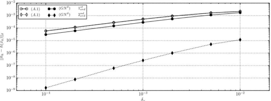
10−4 ₁₀−3 ₁₀−2 δx 10−9 10−8 10−7 10−6 10−5 10−4 10−3 10−2 k hk − h (xk )kδ (A.1) (A.1) (GNδ_{) 1}st ord (GNδ_{) 2}nd ord

Figure 3: §4.1Solitary waves – L2-error of the numerical approximations (A.1) and (G Nδ), with and without the “second order” strategy, as function of the space step at time t = 50.

solution when ∇φ = 0. More precisely, the solitary waves of (N H) and (G N) read

(29) h (t , x) = h 0 (x) = H0+ A sech2 Ãs γXX_A A + H0 x H0 ! and u (t , x) = u0(x) = H0 h0_(x)pg (H0+ A)

with H0> 0 is the water depth far from the wave and A > 0 is the wave elevation. The

parameterγXX_{depend on the model, i.e.γ}NH

= 1 and γGN

=34. The vertical velocity

and the hydrodynamic pressure can be deduce using the compatibility conditions (8) and (21).

In the current section, the convergence rate of the schemes (G Nδ) and (A.1) is illustrated in the simulation of the solitary wave (29). More precisely we set the pa-rameters

H0= 5 · 10−2 and A = 5 · 10−3.

The computational domain is set to [−1,1]. At the left boundary, the discharged is imposed and set to h (t , −1)u (t,−1) = h0(−1)u0(−1) and at the right the water depth is imposed and set to h (t , 1) = h0_(1).

In Figure2, the numerical solutions of the schemes, entropic (G Nδ) and com-pact (A.1), first order and “second order”, are plotted at time t = 50 for some space steps. For small enough space step, the solitary wave is well preserved by every schemes. The convergence rate, illustrated in Figure3, is almost first order for all the schemes except for the “second order” (G Nδ) scheme, The convergence rate, illus-trated in Figure3, is almost one for all schemes except for the “second order” (G Nδ) scheme for which it is almost two as expected. Note the “second order” strategy does not improve the result of the compact scheme (A.1). This is because the dispersion step (A.1) is not a projection on the setAGN₀ ,n. The same results are observed on the other variables u, w andσ and applying the scheme to the non-hydrostatic model

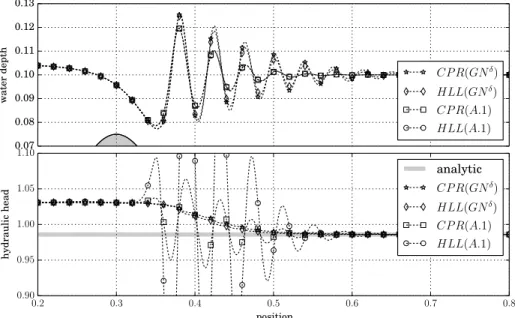
0.07 0.08 0.09 0.10 0.11 0.12 0.13 w at er de pt h CP R(GNδ₎ HLL(GNδ₎ CP R(A.1) HLL(A.1) 0.2 0.3 0.4 0.5 0.6 0.7 0.8 position 0.90 0.95 1.00 1.05 1.10 hy dr au lic he ad analytic CP R(GNδ₎ HLL(GNδ₎ CP R(A.1) HLL(A.1)

Figure 4: §4.2Undular jump – Water level approximated (first line) and hydraulic

head (second line) for several schemes.

(N Hδ).

4.2 Undular jump

A typical test case of (SW) is the transcritical stationary solution in one dimensional framework, see [8]. An analytical solution is based on the energy conservation prop-erty, i.e. Hypothesis2.ii). More precisely, the energy conservation implies that the hydraulic head, defined by the ratio of energy flow to mass flow, i. e.

KSW :=G h + Gu hu = φ + g h + ¯ ¯u ¯ ¯ 2 2 ,

is piecewise constant. At the discontinuities, the jump should satisfy the Rankine-Hugoniot relation, see [8] for details. Using the same arguments, the hydraulic head of the dispersive models (N H) and (G N) respectively given by

KNH :=G h + Gu+Gw+GqB hu = φ + g h + ¯ ¯u ¯ ¯ 2 2 + ¯ ¯w ¯ ¯ 2 2 + qB 2 and KGN :=G h + Gu+Gw+Gσ+ Gq hu = φ + g h + ¯ ¯u ¯ ¯ 2 2 + ¯ ¯w ¯ ¯ 2 2 + |σ|2 2 + q are constant (there is no discontinuity for the dispersive models). Unfortunately, it is not possible to recover the water depth form the hydraulic head as it is for (SW). However, it is possible to compare the hydraulic head of the computed so-lution to the analytical value. The entropy-stability of the scheme is illustrated by

the monotony of the hydraulic head at steady state.

Let us describe the test case more precisely. We consider the computational do-main [0, 1] with an imposed discharged at the left bound h (t , 0) u (t , 0) = 10−2and an imposed water depth at the right bound h (t , 1) = 10−1. The bottom and the surface pressure are set to

B (x) = 7.5 · 10−2e−102(x−0.3)2 and P (x) = 0.

Note that the converged solution is out of reach. More precisely, the better the res-olution, the more oscillations extend to the right. The converged solution presents periodic oscillations at the right of the obstacle which does not decrease in ampli-tude. Thus for a fine enough resolution, the right boundary condition (fixed water depth) is no more relevant and more elaborated boundary condition are required (fixed hydraulic head). Unfortunately, it is not clear how to prescribe it at the dis-crete level.

In Figure4, the water level and the hydraulic head computed with several schemes

Y Y Y¡X Xδ¢ are plotted forδx= 10−4. The schemes Y Y Y refer to the advection step.

The C P R (Centered Potential Regularization) scheme [31] is entropy-satisfying, i.e. it satisfies Hypothesis1.ii), whereas the H LL scheme with hydrostatic reconstruc-tion satisfies only a semi-discrete counterpart of Hypothesis1.ii). The schemes¡X Xδ¢ refer to the dispersive step. (G Nδ) is entropy-satisfying, see Proposition7.ii), con-trary to (A.1). Only the solution C P R(G Nδ) is fully entropy-satisfying and in practice, it is the most accurate. However, the solution of H LL(G Nδ) is almost similar. For this both scheme, the hydraulic head is decreasing as a consequence of the mechanical energy dissipation. In the case of (A.1), the hydraulic head does not decrease, the mechanical energy is not well dissipated and the results are significantly less accu-rate. The impact on the water level is a strong numerical diffusion for both Y Y Y schemes where the hydrodynamic effects occur.

4.3 Water drop

The following test case is devoted to the parametric analysis of the aspect ratio. More precisely, (SW) is known as to be a good approximation of (E) when the aspect ratio

ε is small enough. We propose to compare the dispersive model (N H) and (G N) to (SW) with respect toε.

Let us describe the case precisely. The computational domain is set to [0, 1] and the boundary conditions are walls (symmetric flow). There is no forcing ∇φ = 0 and the initial condition is set to

h0(x) = ε³1 + e−100x2´ and u0(x) = 0.

In Figure5, the water depth approximated by each models withδx= 10−6is

plot-ted for several aspect ratio. The numerical diffusion probably significantly affect the solution forε ≤ 2 · 10−4. The solution of the dispersive models (N H) and (G N) are very similar, i.e. the solutions present a dispersive shock with oscillations of about

1.0 1.5 2.0 ǫ = 5. 10 − 2 1.0 1.5 2.0 ǫ = 2. 10 − 2 1.0 1.5 2.0 ǫ = 1. 10 − 2 1.0 1.5 2.0 ǫ = 5. 10 − 3 1.0 1.5 2.0 ǫ = 2. 10 − 3 1.0 1.5 2.0 ǫ = 1. 10 − 3 1.0 1.5 2.0 ǫ = 5. 10 − 4 1.0 1.5 2.0 ǫ = 2. 10 − 4 0.5 0.6 0.7 0.8 0.9 position 1.0 1.5 2.0 ǫ = 1. 10 − 4 (SWδ_{) (N H}δ₎ 0.5 0.6 0.7 0.8 0.9 position (SWδ_{) (GN}δ₎

Figure 5: §4.3Water drop – Rescaled water depthh/_εapproximated at the rescaled timepgεt = 0.6 by (N Hδ) (left column) and (G Nδ) (right column) for several aspect ratio.

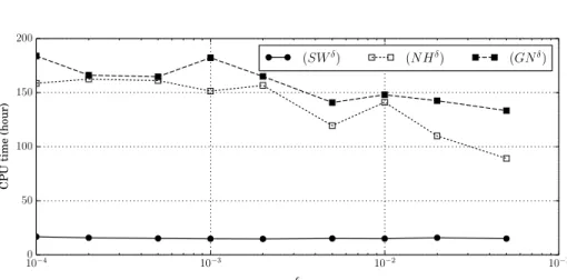
twice the amplitude of the shallow water discontinuity. The frequency is slightly higher for (N H) than for (G N) even if the shape of the convexe hull is the same, i.e. linear with almost the same slope. The smaller theε, the higher the frequency of the oscillation. In Figure6, the CPU time for each simulations in given. The slightly

10−4 ₁₀−3 ₁₀−2 ₁₀−1 ǫ 0 50 100 150 200 C P U ti m e (h ou r) (SWδ_{) (N H}δ_{) (GN}δ₎

Figure 6: §4.3Water drop – CPU time of the hierarchy of models to reach the rescaled

timepgεt = 0.6 for several aspect ratio.

larger CPU time of (G Nδ) can be explain by the advection of the standard deviation.

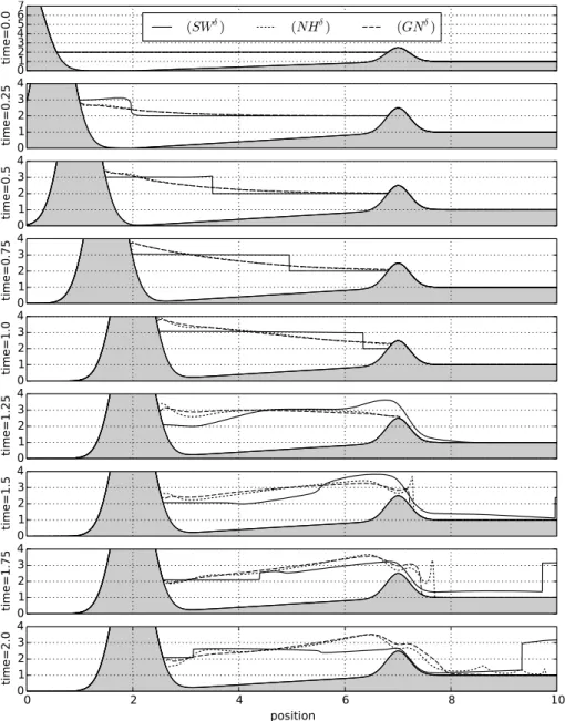
4.4 Seawall

To illustrate the robustness of the numerical strategy for moving bottom and with the dry front, the test case of the seawall is presented. The computational domain is set to [0, 10] and the boundary conditions are walls. The surface pressure is ne-glected P = 0 but the bottom is a time and space function given by

B (t , x) = max(0,min(0.2(x − 2),1)) + 1.5e−10∗(x−7)2+ 10e−5(x−min(2t ,2))2 and the initial condition reads

h0_{(x) =}½max (0, 2 − B (0, x)) if x ≤ 7

0 elsewhere and u

0

(x) = 0.

In Figure7, the water level approximated with H LL¡X Xδ¢ with X X ∈ {N H,GN} andδx= 10−3is plotted at several times. Even if the two dispersive models lead to

significantly different results, especially in the dry front, they are qualitatively sim-ilar. First, we find that the dispersive models and (SW) react very differently to the bottom elevation, i.e. 0 ≤ t < 1. In the case of (SW), the water level does not become much higher than the initial condition, i.e. 3, and a wave is quickly generated. In the case of dispersive models, the water level becomes higher, i.e. it reaches 4, and the beginning of the wave is not as clear. All models pass the dike, but the shape of the free surface is different. In the case of (SW), the free surface is discontinuous before the dike and continuous after, whereas for dispersive models the free surface is con-tinuous before the dike and disconcon-tinuous at the dry front, at least for a while. More precisely, a spike appears at the dry front for a time after the dike and it is clearly not a numerical instability. It was check that this spike is not very sensitive the velocity in the dry cell. We recall that the velocity in the dry cell is set to zero to impose the