Computer Science and Artificial Intelligence Laboratory
Technical Report
MIT-CSAIL-TR-2009-058
November 10, 2009
Distributed Computation in Dynamic Networks
Distributed Computation in Dynamic Networks : Technical
Report
Fabian Kuhn1 Nancy Lynch2 Rotem Oshman2
[email protected] [email protected] [email protected]
1Faculty of Informatics, University of Lugano, 6904 Lugano, Switzerland 2Computer Science and Artificial Intelligence Lab, MIT, Cambridge, MA 02139, USA
Abstract
In this paper we investigate distributed computation in dynamic networks in which the network topology changes from round to round. We consider a worst-case model in which the communication links for each round are chosen by an adversary, and nodes do not know who their neighbors for the current round are before they broadcast their messages. The model allows the study of the fundamental computation power of dynamic networks. In particular, it captures mobile networks and wireless networks, in which mobility and interference render communication unpredictable. In contrast to much of the existing work on dynamic networks, we do not assume that the network eventually stops changing; we require correctness and termination even in networks that change continually. We introduce a stability property called
𝑇 -interval connectivity (for 𝑇 ≥ 1), which stipulates that for every 𝑇 consecutive rounds there
exists a stable connected spanning subgraph. For𝑇 = 1 this means that the graph is connected
in every round, but changes arbitrarily between rounds. Algorithms for the dynamic graph model must cope with these unceasing changes.
We show that in 1-interval connected graphs it is possible for nodes to determine the size of the network and compute any computable function of their initial inputs in𝑂(𝑛2) rounds using
messages of size𝑂(log 𝑛 + 𝑑), where 𝑑 is the size of the input to a single node. Further, if the
graph is𝑇 -interval connected for 𝑇 > 1, the computation can be sped up by a factor of 𝑇 , and
any function can be computed in𝑂(𝑛+𝑛2/𝑇 ) rounds using messages of size 𝑂(log 𝑛+𝑑). We
also give two lower bounds on the gossip problem, which requires the nodes to disseminate𝑘
pieces of information to all the nodes in the network. We show anΩ(𝑛 log 𝑘) bound on gossip
in 1-interval connected graphs against centralized algorithms, and anΩ(𝑛 + 𝑛𝑘/𝑇 ) bound on
exchanging𝑘 pieces of information in 𝑇 -interval connected graphs for a restricted class of
randomized distributed algorithms.
The T-interval connected dynamic graph model is a novel model, which we believe opens new avenues for research in the theory of distributed computing in wireless, mobile and dy-namic networks.
1
Introduction
The study of dynamic networks has gained importance and popularity over the last few years. Driven by the growing ubiquity of the Internet and a plethora of mobile devices with communica-tion capabilities, novel distributed systems and applicacommunica-tions are now within reach. The networks in which these applications must operate are inherently dynamic; typically we think of them as being large and completely decentralized, so that each node can have an accurate view of only its local vicinity. Such networks change over time, as nodes join, leave, and move around, and as communication links appear and disappear.
In some networks, e.g., peer-to-peer, nodes participate only for a short period of time, and the topology can change at a high rate. In wireless ad-hoc networks, nodes are mobile and move around unpredictably. Much work has gone into developing algorithms that are guaranteed to work in networks that eventually stabilize and stop changing; this abstraction is unsuitable for reasoning about truly dynamic networks.
The objective of this paper is to make a step towards understanding the fundamental possibili-ties and limitations for distributed algorithms in dynamic networks in which eventual stabilization of the network is not assumed. We introduce a general dynamic network model, and study com-putability and complexity of essential, basic distributed tasks. Under what conditions is it possible to elect a leader or to compute an accurate estimate of the size of the system? How efficiently can information be disseminated reliably in the network? To what extent does stability in the commu-nication graph help solve these problems? These and similar questions are the focus of our current work.
The dynamic graph model. In the interest of broad applicability our dynamic network model makes few assumptions about the behavior of the network, and we study it from the worst-case per-spective. In the current paper we consider a fixed set of nodes that operate in synchronized rounds and communicate by broadcast. In each round the communication graph is chosen adversarially, under an assumption of𝑇 -interval connectivity: throughout every block of 𝑇 consecutive rounds
there must exist a connected spanning subgraph that remains stable.
We consider the range from 1-interval connectivity, in which the communication graph can change completely from one round to the next, to∞-interval connectivity, in which there exists
some stable connected spanning subgraph that is not known to the nodes in advance. We note that edges that do not belong to the stable subgraph can still change arbitrarily from one round to the next, and nodes do not know which edges are stable and which are not. We do not assume that a neighbor-discovery mechanism is available to the nodes; they have no means of knowing ahead of time which nodes will receive their message.
In this paper we are mostly concerned with deterministic algorithms, but our lower bounds cover randomized algorithms as well. The computation model is as follows. In every round, the adversary first chooses the edges for the round; for this choice it can see the nodes’ internal states at the beginning of the round. At the same time and independent of the adversary’s choice of edges, each node tosses private coins and uses them to generate its message for the current round. Deterministic algorithms generate the message based on the interal state alone. In both cases the nodes do not know which edges were chosen by the advesary. Each message is then delivered to
the sender’s neighbors, as chosen by the adversary; the nodes transition to new states, and the next round begins. Communication is assumed to be bidirectional, but this is not essential. We typically assume that nodes know nothing about the network, not even its size, and communication is limited to𝑂(log 𝑛) bits per message.
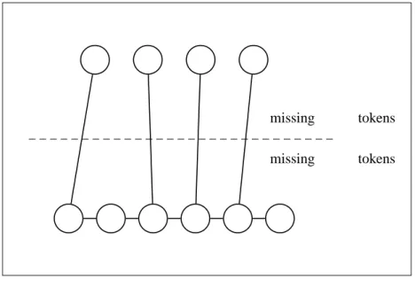
To demonstrate the power of the adversary in the dynamic graph model, consider the problem of
local token circulation: each node𝑢 has a local Boolean variable token𝑢, and if token𝑢 = 1, node
𝑢 is said to “have the token”. In every round exactly one node in the network has the token, and it
can either keep the token or pass it to one of its neighbors. The goal is for all nodes to eventually have the token in some round. This problem is impossible to solve in 1-interval connected graphs: in every round, the adversary can see which node𝑢 has the token, and provide that node with only
one edge {𝑢, 𝑣}. Node 𝑢 then has no choice except to eventually pass the token to 𝑣. After 𝑣
receives it, the adversary can turn around and remove all of𝑣’s edges except {𝑢, 𝑣}, so that 𝑣 has
no choice except to pass the token back to𝑢. In this way the adversary can prevent the token from
ever visiting any node except𝑢, 𝑣.
Perhaps surprisingly given our powerful adversary, even in 1-interval connected graphs it is possible to reliably compute any computable function of the initial states of the nodes, and even have all nodes output the result at the same time (simultaneity).
The dynamic graph model we suggest can be used to model various dynamic networks. Perhaps the most natural scenario is mobile networks, in which communication is unpredictable due to the mobility of the agents. There is work on achieving continual connectivity of the communication graph in this setting (e.g., [12]), but currently little is known about how to take advantage of such a service. The dynamic graph model can also serve as an abstraction for static or dynamic wireless networks, in which collisions and interference make it difficult to predict which messages will be delivered, and when. Finally, dynamic graphs can be used to model traditional communication net-works, replacing the traditional assumption of a bounded number of failures with our connectivity assumption.
Although we assume that the node set is static, this is not a fundamental limitation. We defer in-depth discussion to future work; however, our techniques are amenable to standard methods such as logical time, which could be used to define the permissible outputs for a computation with a dynamic set of participants.
Contribution. In this paper we mainly study the following problems in the context of dynamic graphs.
∙ Counting, in which nodes must determine the size of the network.
∙ 𝑘-gossip, in which 𝑘 pieces of information, called tokens, are handed out to some nodes in
the network, and all nodes must collect all𝑘 tokens.
We are especially interested in the variant of𝑘-gossip where the number of tokens is equal to the
number of nodes in the network, and each node starts with exactly one token. This variant of gossip allows any function of the initial states of the nodes to be computed. However, it requires counting, since nodes do not know in advance how many tokens they need to collect. We show that both problems can be solved in𝑂(𝑛2) rounds in 1-interval connected graphs. Then we extend the
algorithm for𝑇 -interval connected graphs with known 𝑇 > 1, obtaining an 𝑂(𝑛 + 𝑛2/𝑇 )-round
protocol for counting or all-to-all gossip. When𝑇 is not known, we show that both problems can
be solved in𝑂(min{𝑛2, 𝑛 + 𝑛2log 𝑛/𝑇}) rounds.
We also give two lower bounds, both concerning token-forwarding algorithms for gossip. A
token-forwarding algorithm is one that does not combine or alter tokens, only stores and forwards
them. First, we give anΩ(𝑛 log 𝑘) lower bound on 𝑘-gossip in 1-interval connected graphs. This
lower bound holds even against centralized algorithms, in which each node is told which token to broadcast by some central authority that can see the entire state of the network. We also give an Ω(𝑛 + 𝑛𝑘/𝑇 ) lower bound on 𝑘-gossip in 𝑇 -interval connected graphs for a restricted class
of randomized algorithms, in which the nodes’ behavior depends only on the set of tokens they knew in each round up to the current one. This includes the algorithms in the paper, as well as other natural strategies such as round robin, choosing a token to broadcast uniformly at random, or assigning a probability to each token that depends on the order in which the tokens were learned.
For simplicity, the results we present here assume that all nodes start the computation in the same round. It is generally not possible to solve any non-trivial problem if some nodes are initially asleep and do not participate. However, if 2-interval connectivity is assumed, it becomes possible to solve𝑘-gossip and counting even when computation is initiated by one node and the rest of the
nodes are asleep.
Related work. For static networks, information dissemination and basic network aggregation tasks have been extensively studied (see e.g. [5, 16, 29]). In particular, the 𝑘-gossip problem is
analyzed in [35], where it is shown that𝑘 tokens can always be broadcast in time 𝑂(𝑛 + 𝑘) in
a static graph. The various problems have also been studied in the context of alternative com-munication models. A number of papers look at the problem of broadcasting a single message (e.g. [8, 23]) or multiple messages [11, 26] in wireless networks. Gossiping protocols are an-other style of algorithm in which it is assumed that in each round each node communicates with a small number of randomly-chosen neighbors. Various information dissemination problems for the gossiping model have been considered [17, 19, 21]; gossiping aggregation protocols that can be used to approximate the size of the system are described in [20, 31]. The gossiping model differs from our dynamic graph model in that the neighbors for each node are chosen at random and not adversarially, and in addition, pairwise interaction is usually assumed where we assume broadcast. A dynamic network topology can arise from node and link failures; fault tolerance, i.e., re-silience to a bounded number of faults, has been at the core of distributed computing research from its very beginning [5, 29]. There is also a large body of previous work on general dy-namic networks. However, in much of the existing work, topology changes are restricted and assumed to be “well-behaved” in some sense. One popular assumption is eventual stabilization (e.g., [1, 6, 7, 36, 18]), which asserts that changes eventually stop occuring; algorithms for this set-ting typically guarantee safety throughout the execution, but progress is only guaranteed to occur after the network stabilizes. Self-stabilization is a useful property in this context: it requires that the system converge to a valid configuration from any arbitrary starting state. We refer to [13] for a comprehensive treatment of this topic. Another assumption, studied for example in [22, 24, 30], requires topology changes to be infrequent and spread out over time, so that the system has enough
reversal [14], an algorithm for maintaining routes in a dynamic topology, as a building block. Protocols that work in the presence of continual dynamic changes have not been widely studied. There is some work on handling nodes that join and leave continually in peer-to-peer overlay networks [15, 27, 28]. Most closely related to the problems studied here is [32], where a few basic results in a similar setting are proved; mainly it is shown that in 1-interval connected dynamic
graphs (the definition in [32] is slightly different), if nodes have unique identifiers, it is possible to globally broadcast a single message and have all nodes eventually stop sending messages. The time complexity is at least linear in the value of the largest node identifier. In [2], Afek and Hendler give lower bounds on the message complexity of global computation in asynchronous networks with arbitrary link failures.
A variant of𝑇 -interval connectivity was used in [25], where two of the authors studied clock
synchronization in asynchronous dynamic networks. In [25] it is assumed that the network satisfies
𝑇 -interval connectivity for a small value of 𝑇 , which ensures that a connected subgraph exists
long enough for each node to send one message. This is analogous to 1-interval connectivity in synchronous dynamic networks.
The time required for global broadcast has been studied in a probabilistic version of the edge-dynamic graph model, where edges are independently formed and removed according to simple Markovian processes [9, 10]. Similar edge-dynamic graphs have also been considered in control theory literature, e.g. [33, 34].
Finally, a somewhat related computational model is population protocols, introduced in [3], where the system is modeled as a collection of finite-state agents with pairwise interactions. Pop-ulation protocols typically (but not always) rely on a strong fairness assumption which requires every pair of agents to interact infinitely often in an infinite execution. We refer to [4] for a sur-vey. Unlike our work, population protocols compute some function in the limit, and nodes do not know when they are done; this can make sequential composition of protocols challenging. In our model nodes must eventually output the result of the computation, and sequential composition is straightforward.
2
Network Model
2.1 Dynamic Graphs
A synchronous dynamic network is modelled by a dynamic graph𝐺 = (𝑉, 𝐸), where 𝑉 is a static
set of nodes, and𝐸 : ℕ → 𝑉(2)is a function mapping a round number𝑟 ∈ ℕ to a set of undirected
edges𝐸(𝑟). Here 𝑉(2):= {{𝑢, 𝑣} ∣ 𝑢, 𝑣 ∈ 𝑉 } is the set of all possible undirected edges over 𝑉 .
Definition 2.1 (𝑇 -Interval Connectivity). A dynamic graph 𝐺 = (𝑉, 𝐸) is said to be 𝑇 -interval
connected for𝑇 ∈ ℕ if for all 𝑟 ∈ ℕ, the static graph 𝐺𝑟,𝑇 :=
(
𝑉,∩𝑟+𝑇 −1
𝑖=𝑟 𝐸(𝑟)
)
is connected. If
𝐺 is 1-interval connected we say that 𝐺 is always connected.
Definition 2.2 (∞-Interval Connectivity). A dynamic graph 𝐺 = (𝑉, 𝐸) is said to be ∞-interval
Note that even though in an ∞-interval connected graph there is some stable subgraph that
persists throughout the execution, this subgraph is not known in advance to the nodes, and can be chosen by the adversary “in hindsight”.
Although we are generally interested in the undirected case, it is also interesting to consider
directed dynamic graphs, where the communication links are not necessarily symmetric. The𝑇
-interval connectivity assumption is then replaced by𝑇 -interval strong connectivity, which requires
that𝐺𝑟,𝑇 be strongly connected (where𝐺𝑟,𝑇 is defined as before). In this very weak model, not
only do nodes not know who will receive their message before they broadcast, they also do not know who received the message after it is broadcast. Interestingly, all of our algorithms for the undirected case work in the directed case as well.
The causal order for dynamic graphs is defined in the standard way.
Definition 2.3 (Causal Order). Given a dynamic graph 𝐺 = (𝑉, 𝐸), we define an order →⊆ (𝑉 × ℕ)2, where (𝑢, 𝑟) → (𝑣, 𝑟′) iff 𝑟′ = 𝑟 + 1 and {𝑢, 𝑣} ∈ 𝐸(𝑟). The causal order ⇝⊆
(𝑉 × ℕ)2 is the reflexive and transitive closure of →. We also write 𝑢 ⇝ (𝑣, 𝑟) if there exists
some𝑟′ ≤ 𝑟 such that (𝑢, 𝑟′) ⇝ (𝑣, 𝑟).
Definition 2.4 (Influence Sets). We denote by𝐶𝑢(𝑟 ⇝ 𝑟′) := {𝑣 ∈ 𝑉 ∣ (𝑣, 𝑟) ⇝ (𝑢, 𝑟′)} the set
of nodes whose state in round𝑟 causally influences node 𝑢 in round 𝑟′. We also use the short-hand
𝐶𝑢(𝑟) := 𝐶𝑢(0 ⇝ 𝑟) = {𝑣 ∣ 𝑣 ⇝ (𝑢, 𝑟)}.
2.2 Communication and Adversary Model
Nodes communicate with each other using anonymous broadcast, with message sizes limited to
𝑂(log(𝑛)). At the beginning of round 𝑟, each node 𝑢 decides what message to broadcast based on
its internal state and private coin tosses; at the same time and independently, the adversary chooses a set𝐸(𝑟) of edges for the round. For this choice the adversary can see the nodes’ internal states at
the beginning of the round, but not the results of their coin tosses or the message they have decided to broadcast. (Deterministic algorithms choose a message based only on the internal state, and this is equivalent to letting the adversary see the message before it chooses the edges.) The adversary then delivers to each node𝑢 all messages broadcast by nodes 𝑣 such that {𝑢, 𝑣} ∈ 𝐸(𝑟). Based on
these messages, its previous internal state, and possibly more coin tosses, the node transitions to a new state, and the round ends. We call this anonymous broadcast because nodes do not know who will receive their message prior to broadcasting it.
2.3 Sleeping Nodes
Initially all nodes in the network are asleep; computation begins when a subset of nodes, chosen by the adversary, is woken up. Sleeping nodes remain in their initial state and do not broadcast any messages until they receive a message from some awake node or are woken up by the adversary. Then they wake up and begin participating in the computation; however, since messages are deliv-ered at the end of the round, a node that is awakened in round𝑟 sends its first message in round 𝑟 + 1.
2.4 Initial Knowledge
Each node in the network starts execution of the protocol in an initial state which contains its own ID, its input, and possibly additional knowledge about the network. We generally assume one of the following.
∙ No knowledge: nodes know nothing about the network, and initially cannot distinguish it
from any other network.
∙ Upper bound on size: nodes know some upper bound 𝑁 on the size 𝑛 of the network. The
upper bound is assumed to be bounded by some function of the true size, e.g.,𝑁 = 𝑂(𝑛). ∙ Exact size: nodes know the size 𝑛 of the network.
2.5 Computation Model
We think of each node in the network as running a specialized Turing machine which takes the node’s UID and input from its input tape at the beginning of the first round, and in subsequent rounds reads the messages delivered to the node from the input tape. In each round the machine produces a message to broadcast on an output tape. On a separate output tape, it eventually writes the final output of the node, and then enters a halting state.
The algorithms in this paper are written in pseudo-code. We use𝑥𝑢(𝑟) to denote the value of
node𝑢’s local variable 𝑥 at the beginning of round 𝑟, and 𝑥𝑢(0) to denote the input to node 𝑢.
3
Problem Definitions
We assume that nodes have unique identifiers (UIDs) from some namespace𝒰. Let 𝒟 be a problem
domain. Further, let𝐴 7→ 𝐵 denote the set of all partial functions from 𝐴 to 𝐵.
A problem over 𝒟 is a relation 𝑃 ⊆ (𝒰 7→ 𝒟)2, such that if (𝐼, 𝑂) ∈ 𝑃 then domain(𝐼) is
finite anddomain(𝐼) = domain(𝑂). Each instance 𝐼 ∈ 𝒰 7→ 𝒟 induces a set 𝑉 = domain(𝐼) of
nodes, and we say that an algorithm solves instance𝐼 if in any dynamic graph 𝐺 = (𝑉, 𝐸), when
each node𝑢 ∈ 𝑉 starts with 𝐼(𝑢) as its input, eventually each node outputs a value 𝑂(𝑢) ∈ 𝒟 such
that(𝐼, 𝑂) ∈ 𝑃 .
We are interested in the following problems.
Counting. In this problem the nodes must determine the size of the network. Formally, the counting problem is given by
counting:= {(𝑉 × {1} , 𝑉 × {𝑛}) ∣ 𝑉 is finite and 𝑛 = ∣𝑉 ∣} .
𝒌-Verification. Closely related to counting, in the𝑘-verification problem nodes are given an
inte-ger𝑘 and must determine whether or not 𝑘 ≥ 𝑛, eventually outputting a Boolean value. Formally, k-verification:= {(𝑉 × {𝑘} , 𝑉 × {𝑏}) ∣ 𝑏 ∈ {0, 1} and 𝑏 = 1 iff 𝑘 ≥ ∣𝑉 ∣} .
𝒌-Committee. In this problem the nodes must form sets (“committees”), where each committee has a unique identifier that is known to all its members. Each node𝑢 outputs a value committee𝑢,
and we require the following properties.
1. (“Safety”) The size of each committee is at most𝑘, that is, for all 𝑥 ∈ {committee𝑢∣ 𝑢 ∈ 𝑉 }
we have∣ {𝑢 ∈ 𝑉 ∣ committee𝑢 = 𝑥} ∣ ≤ 𝑘.
2. (“Liveness”) If𝑘 ≥ 𝑛 then all nodes in the graph join one committee, that is, for all 𝑢, 𝑣 ∈ 𝑉
we have committee𝑢 = committee𝑣.
𝒌-Gossip. The gossip problem is defined over a token domain𝒯 . Each node receives in its input
a set of tokens, and the goal is for all nodes to output all tokens. Formally,
k-gossip:= {(𝑉 → 𝒫 (𝐴) , 𝑉 → 𝐴) ∣ 𝑉 is finite and ∣𝐴∣ = 𝑘} .
We are particularly interested in the following variants of the problem.
∙ All-to-All gossip: instances 𝐼 where 𝑘 = 𝑛 for all 𝑢 ∈ 𝑉 we have ∣𝐼(𝑢)∣ = 1.
∙ 𝑘-gossip with known 𝑘: in this variant nodes know 𝑘, i.e., they receive 𝑘 as part of the input.
Leader Election. In weak leader election all nodes must eventually output a bit 𝑏, such that
exactly one node outputs 𝑏 = 1. In strong leader election, all nodes must output the same ID 𝑢 ∈ 𝑉 of some node in the network.
4
Relationships
A problem𝑃1 is reducible to𝑃2 if whenever all nodes start the computation in initial states that
represent a solution to𝑃2, there is an algorithm that computes a solution to𝑃1 and requires linear
time in the parameter to the problem (𝑘).
4.1 𝒌-Committee ≡ 𝒌-Verification
Claim 4.1. 𝑘-verification reduces to 𝑘-committee.
Proof. Suppose we start from a global state that is a solution to𝑘-committee, that is, each node 𝑢
has a local variable committee𝑢 such that at most𝑘 nodes belong to the same committee, and if
𝑘 ≥ 𝑛 then all nodes belong to one committee. We can verify whether or not 𝑘 ≥ 𝑛 as follows. For 𝑘 rounds, each node maintains a Boolean flag 𝑏, which is initially set to 1. In rounds where 𝑏 = 1,
the node broadcasts its committee ID, and when𝑏 = 0 the node broadcasts ⊥. If a node receives a
committee ID different from its own, or if it hears the special value⊥, it sets 𝑏 to 0. At the end of
the𝑘 rounds all nodes output 𝑏.
First consider the case where𝑘 ≥ 𝑛. In this case all nodes have the same committee ID, and
suppose that𝑘 < 𝑛, and let 𝑢 be some node. There are at most 𝑘 − 1 nodes in 𝑢’s committee. In
every round, there is an edge between some node in𝑢’s committee and some node in a different
committee (because the communication graph is connected), and therefore at least one node in𝑢’s
committee sets its𝑏 flag to 0. After at most 𝑘 rounds no nodes remain, and in particular 𝑢 itself
must have𝑏𝑢 = 0. Thus, at the end of the protocol all nodes output 0.
Claim 4.2. 𝑘-committee reduces to 𝑘-verification.
Proof. Again, suppose the nodes are initially in a state that represents a solution to𝑘-verification:
they have a Boolean flag𝑏 which is set to 1 iff 𝑘 ≥ 𝑛. We solve 𝑘-committee as follows: if 𝑏 = 0,
then each node outputs its own ID as its committee ID. This is a valid solution because when𝑘 < 𝑛
the only requirement is that no committee have more than𝑘 nodes. If 𝑏 = 1, then for 𝑘 rounds
all nodes broadcast the minimal ID they have heard so far, and at the end they output this ID as their committee ID. Since𝑏 = 1 indicates that 𝑘 ≥ 𝑛, after 𝑘 rounds all nodes have heard the
ID of the node with the minimal ID in the network, and they will all join the same committee, as required.
4.2 Counting vs.𝒌-Verification
Since we can solve𝑘-verification in 𝑂(𝑘 + 𝑘2/𝑇 ) time in 𝑇 -interval connected graphs, we can find
an upper bound on the size of the network by checking whether𝑘 ≥ 𝑛 for values of 𝑘 starting from
1 and doubling with every wrong guess. We know how to verify whether𝑘 ≥ 𝑛 in 𝑂(𝑘 + 𝑘2/𝑇 )
time, and hence the time complexity of the entire procedure is𝑂(𝑛 + 𝑛2/𝑇 ). Once we establish
that𝑘 ≥ 𝑛 for some value of 𝑘, to get an actual count we can then go back and do a binary search
over the range𝑘/2, . . . , 𝑘 (recall that 𝑘/2 < 𝑛, otherwise we would not have reached the current
value of𝑘).
In practice, we use a variant of𝑘-committee where the ID of each committee is the set
con-taining the IDs of all members of the committee. The𝑘-verification layer returns this set as well,
so that after reaching a value of𝑘 ≥ 𝑛 at node 𝑢, we simply return the size of 𝑢’s committee as
the size of the network. Since𝑘 ≥ 𝑛 implies that all nodes join the same committee, node 𝑢 will
output the correct count.
4.3 Hierarchy of Problems
There is a hardness hierarchy among the problems considered in this paper as well as some other natural problems.
1. Strong leader election / consensus (these are equivalent). 2. Decomposable functions such as Boolean AND / OR 3. Counting.
The problems in every level are reducible to the ones in the next level, and we know that𝑛-gossip
can be solved in𝑂(𝑛 + 𝑛2/𝑇 ) time in 𝑇 -interval connected graphs for 𝑇 ≥ 2, or 𝑇 ≥ 1 assuming
synchronous start. Therefore all the problems can be solved in𝑂(𝑛 + 𝑛2/𝑇 ) time, even with no
prior knowledge of the network, and even when the communication links are directed (assuming strong connectivity).
5
Upper Bounds
In this section we give algorithms for some of the problems introduced in Section 3, always with the goal of solving the counting problem. Our strategy is usually as follows:
1. Solve some variant of gossip.
2. Use (1) as a building block to solve𝑘-committee,
3. Solving𝑘-committee allows us to solve 𝑘-verification and therefore also counting (see
Sec-tion 4).
We initially focus on the case of synchronous start. The modifications necessary to deal with asynchronous start are described in Section 5.5.
5.1 Always-Connected Graphs
5.1.1 Basic Information Dissemination
It is a basic fact that in 1-interval connected graphs, a single piece of information requires at most
𝑛 − 1 rounds to reach all the nodes in the network, provided that it is forwarded by all nodes
that receive it. Formally, let 𝐷𝑢(𝑟) := {𝑣 ∈ 𝑉 ∣ 𝑢 ⇝ (𝑣, 𝑟)} denote the set of nodes that 𝑢 has
“reached” by round𝑟. If 𝑢 knows a token and broadcasts it constantly, and all other nodes broadcast
the token if they know it, then all the nodes in𝐷𝑢(𝑟) know the token by round 𝑟.
Claim 5.1. For any node𝑢 and round 𝑟 ≤ 𝑛 − 1 we have ∣𝐷𝑢(𝑟)∣ ≥ 𝑟 + 1.
Proof. By induction on𝑟. For 𝑟 = 0 the claim is immediate. For the step, suppose that ∣𝐷𝑢(𝑟)∣ ≥
𝑟 + 1, and consider round 𝑟 + 1 ≤ 𝑛. If 𝐷𝑢(𝑟) = 𝑉 then the claim is trivial, because 𝐷𝑢(𝑟) ⊆
𝐷𝑢(𝑟 + 1). Thus, suppose that 𝐷𝑢(𝑟) ∕= 𝑉 . Since 𝐺(𝑟) is connected, there is some edge {𝑥, 𝑦}
in the cut(𝐷𝑢(𝑟), 𝑉 ∖ 𝐷𝑢(𝑟)). From the definition of the causal order we have 𝑥, 𝑦 ∈ 𝐷𝑢(𝑟 + 1),
and therefore∣𝐷𝑢(𝑟 + 1)∣ ≥ ∣𝐷𝑢(𝑟)∣ + 1 ≥ 𝑟 + 2.
Note that we can employ this property even when there is more than one token in the network, provided that tokens form a totally-ordered set and nodes forward the smallest (or biggest) token they know. It is then guaranteed that the smallest (resp. biggest) token in the network will be known by all nodes after at most𝑛 − 1 rounds. Note, however, that in this case nodes do not necessarily
5.1.2 Counting in linear time withΩ(𝒏 log 𝒏)-bit messages
We begin by describing a linear-time counting/𝑛-gossip protocol which uses messages of size Ω(𝑛 log 𝑛). The protocol is extremely simple, but it demonstrates some of the ideas used in some
of our later algorithms, where we eliminate the large messages using a stability assumption (𝑇
-interval connectivity) which allows nodes to communicate with at least one of their neighbors for at least𝑇 rounds.
In the simple protocol, all nodes maintain a set𝐴 containing all the IDs (or tokens) they have
collected so far. In every round, each node broadcasts 𝐴 and adds any IDs it receives. Nodes
terminate when they first reach a round𝑟 in which ∣𝐴∣ < 𝑟. 𝐴 ← {self }
for𝑟 = 1, 2, . . . do
broadcast𝐴
receive𝐵1, . . . , 𝐵𝑠from neighbors
𝐴 ← 𝐴 ∪ 𝐵1∪ . . . ∪ 𝐵𝑠
if∣𝐴∣ < 𝑟 then terminate and output ∣𝐴∣
end
Algorithm 1: Counting in linear time using large messages
Claim 5.2. For any node𝑢 and rounds 𝑟 ≤ 𝑟′≤ 𝑛 we have ∣𝐶𝑢(𝑟 ⇝ 𝑟′)∣ ≥ 𝑟′− 𝑟.
Proof. By induction on𝑟′− 𝑟. For 𝑟′− 𝑟 = 0 the claim is immediate.
Suppose that for all nodes𝑢 and rounds 𝑟, 𝑟′such that𝑟′ ≤ 𝑛 and 𝑟′− 𝑟 = 𝑖 we have ∣𝐶𝑢(𝑟 ⇝
𝑟′)∣ ≥ 𝑖. Let 𝑟, 𝑟′ ≤ 𝑛 be two rounds such that 𝑟′− 𝑟 = 𝑖 + 1.
If∣𝐶𝑢((𝑟 + 1) ⇝ 𝑟)∣ = 𝑛 then we are done, because 𝑟′ − 𝑟 ≤ 𝑟′ ≤ 𝑛. Thus, assume that
𝐶𝑢((𝑟 + 1) ⇝ 𝑟) ∕= 𝑉 . Since the communication graph in round 𝑟 is connected, there is some
edge{𝑤, 𝑤′} ∈ 𝐸(𝑟) such that 𝑤 ∕∈ 𝐶
𝑢((𝑟 + 1) ⇝ 𝑟) and 𝑤′ ∈ 𝐶𝑢((𝑟 + 1) ⇝ 𝑟). We have
(𝑤, 𝑟) → (𝑤′, 𝑟 + 1) ⇝ (𝑢, 𝑟′), and consequently (𝑤, 𝑟) ⇝ (𝑢, 𝑟′) and 𝑤 ∈ 𝐶
𝑢(𝑟 ⇝ 𝑟′). Also,
from the induction hypothesis, ∣𝐶𝑢((𝑟 + 1) ⇝ 𝑟)∣ ≥ 𝑖. Together we obtain ∣𝐶𝑢(𝑟 ⇝ 𝑟′)∣ ≥
∣𝐶𝑢((𝑟 + 1) ⇝ 𝑟)∣ + 1 ≥ 𝑖 + 1, as desired.
Claim 5.3. For any node𝑢 and round 𝑟 ≤ 𝑛 we have ∣𝐴𝑢(𝑟)∣ ≥ 𝑟.
Proof. It is easily shown that for all𝑣 ∈ 𝐶𝑢(𝑟) we have 𝑣 ∈ 𝐴𝑢(𝑟). From the previous claim we
have∣𝐶𝑢(𝑟)∣ ≥ 𝑟 for all 𝑟 ≤ 𝑛, and the claim follows.
The correctness of the protocol follows from Claim 5.3: suppose that for some round 𝑟 and
node𝑢 we have ∣𝐴𝑢(𝑟)∣ < 𝑟. From Claim 5.3, then, 𝑟 > 𝑛. Applying the claim again, we see
that∣𝐴𝑢(𝑛)∣ ≥ 𝑛, and since 𝐴𝑢(𝑟) ⊆ 𝑉 for all 𝑟, we obtain 𝐴𝑢(𝑟) = 𝑉 . This shows that nodes
compute the correct count. For termination we observe that the size of𝐴𝑢 never exceeds𝑛, so all
5.1.3 𝒌-committee with 𝑶(log 𝒏)-bit messages
We can solve𝑘-committee in 𝑂(𝑘2) rounds as follows. Each node 𝑢 stores a local variable leader𝑢
in addition to committee𝑢. A node that has not yet joined a committee is called active, and a node
that has joined a committee is inactive. Once nodes have joined a committee they do not change their choice.
Initially all nodes consider themselves leaders, but throughout the protocol, any node that hears an ID smaller than its own adopts that ID as its leader. The protocol proceeds in𝑘 cycles, each
consisting of two phases, polling and selection.
1. Polling phase: for𝑘 − 1 rounds, all nodes propagate the ID of the smallest active node of
which they are aware.
2. Selection phase: in this phase, each node that considers itself a leader selects the smallest ID it heard in the previous phase and invites that node to join its committee. An invitation is represented as a pair(𝑥, 𝑦), where 𝑥 is the ID of the leader that issued the invitation, and 𝑦 is the ID of the invited node. All nodes propagate the smallest invitation of which they
are aware for 𝑘 − 1 (invitations are sorted in lexicographic order, so that invitations issued
by the smallest node in the network will win out over other invitations. It turns out, though, that this is not necessary for correctness; it is sufficient for each node to forward an arbitrary invitation from among those it received).
At the end of the selection phase, a node that receives an invitation to join its leader’s com-mittee does so and becomes inactive. (Invitations issued by nodes that are not the current leader can be accepted or ignored; this, again, does not affect correctness.)
At the end of the 𝑘 cycles, any node 𝑢 that has not been invited to join a committee outputs committee𝑢= 𝑢.
leader ← self committee ← ⊥
for𝑖 = 0, . . . , 𝑘 do
// Polling phase
if committee = ⊥ then
min active ← self ; // The node nominates itself for selection
else
min active ← ⊥
end
for𝑗 = 0, . . . , 𝑘 − 1 do
broadcast min active
receive𝑥1, . . . , 𝑥𝑠from neighbors
min active ← min {min active, 𝑥1, . . . , 𝑥𝑠}
end
// Update leader
leader ← min {leader , min active}
// Selection phase
if leader = self then
// Leaders invite the smallest ID they heard
invitation ← (self , min active)
else
// Non-leaders do not invite anybody
invitation ← ⊥
end
for𝑗 = 0, . . . , 𝑘 − 1 do
broadcast invitation
receive𝑦1, . . . , 𝑦𝑠from neighbors
invitation ← min {invitation, 𝑦1, . . . , 𝑦𝑠} ; // (in lexicographic order)
end
// Join the leader’s committee, if invited
if invitation = (leader , self ) then committee = leader end end if committee = ⊥ then committee ← self end
Algorithm 2:𝑘-committee in always-connected graphs
Claim 5.4. The protocol solves the𝑘-committee problem.
Proof. We show that after the protocol ends, the values of the local committee𝑢variables constitute
1. In each cycle, each node invites at most one node to join its committee. After𝑘 cycles at
most 𝑘 nodes have joined any committee. Note that the first node invited by a leader 𝑢 to
join 𝑢’s committee is always 𝑢 itself. Thus, if after 𝑘 cycles node 𝑢 has not been invited to
join a committee, it follows that𝑢 did not invite any other node to join its committee; when
it forms its own committee in the last line of the algorithm, the committee’s size is 1. 2. Suppose that𝑘 ≥ 𝑛, and let 𝑢 be the node with the smallest ID in the network. Following
the polling phase of the first cycle, all nodes 𝑣 have leader𝑣 = 𝑢 for the remainder of
the protocol. Thus, throughout the execution, only node𝑢 issues invitations, and all nodes
propagate 𝑢’s invitations. Since 𝑘 ≥ 𝑛 rounds are sufficient for 𝑢 to hear the ID of the
minimal active node in the network, in every cycle node𝑢 successfully identifies this node
and invites it to join𝑢’s committee. After 𝑘 cycles, all nodes will have joined.
Remark. The protocol can be modified easily to solve𝑛-gossip if 𝑘 ≥ 𝑛. Let 𝑡𝑢 be the token
node𝑢 received in its input (or ⊥ if node 𝑢 did not receive a token). Nodes attach their tokens to
their IDs, and send pairs of the form(𝑢, 𝑡𝑢) instead of just 𝑢. Likewise, invitations now contain the
token of the invited node, and have the structure(leader , (𝑢, 𝑡𝑢)). The min operation disregards
the token and applies only to the ID. At the end of each selection phase, nodes extract the token of the invited node, and add it to their collection. By the end of the protocol every node has been invited to join the committee, and thus all nodes have seen all tokens.
5.2 ∞-interval Connected Graphs
We can count in linear time in∞-interval connected graphs using the following algorithm: each
node maintains two sets of IDs,𝐴 and 𝑆. 𝐴 is the set of all IDs known to the node, and 𝑆 is the
set of IDs the node has already broadcast. Initially𝐴 contains only the node’s ID and 𝑆 is empty.
In every round, each node broadcastsmin (𝐴 ∖ 𝑆) and adds this value to 𝑆. (If 𝐴 = 𝑆, the node
broadcasts nothing.) Then it adds all the IDs it receives from its neighbors to𝐴.
While executing this protocol, nodes keep track of the current round number (starting from zero). When a node reaches a round𝑟 in which ∣𝐴∣ < ⌊𝑟/2⌋, it terminates and outputs ∣𝐴∣ as the
𝑆 ← ∅ 𝐴 ← {self } for𝑟 = 0, . . . do if𝑆 ∕= 𝐴 then 𝑡 ← min (𝐴 ∖ 𝑆) broadcast𝑡 𝑆 ← 𝑆 ∪ {𝑡} end
receive𝑡1, . . . , 𝑡𝑠from neighbors
𝐴 ← 𝐴 ∪ {𝑡1, . . . , 𝑡𝑠}
if∣𝐴∣ < ⌊𝑟/2⌋ then terminate and output ∣𝐴∣
end return𝐴
Algorithm 3: Counting in∞-interval connected graphs
5.2.1 Analysis
Letdist(𝑢, 𝑣) denote the shortest-path distance between 𝑢 and 𝑣 in the stable subgraph 𝐺′, and let
𝑁𝑑(𝑢) denote the 𝑑-neighborhood of 𝑢 in 𝐺′, that is,𝑁𝑑(𝑢) = {𝑣 ∈ 𝑉 ∣ dist(𝑢, 𝑣) ≤ 𝑑}. We use
𝐴𝑥(𝑟) and 𝑆𝑥(𝑟) to denote the values of local variables 𝐴 and 𝑆 at node 𝑥 ∈ 𝑉 in the beginning of
round𝑟. Note the following properties:
1. 𝑆𝑥(𝑟 + 1) ⊆ 𝐴𝑥(𝑟) ⊆ 𝐴𝑥(𝑟 + 1) for all 𝑥 and 𝑟.
2. If𝑢 and 𝑣 are neighbors in 𝐺′, then𝑆
𝑢(𝑟) ⊆ 𝐴𝑣(𝑟) for all 𝑟, because every value sent by 𝑢
is received by𝑣 and added to 𝐴𝑣.
3. 𝑆 and 𝐴 are monotonic, that is, for all 𝑥 and 𝑟 we have 𝑆𝑥(𝑟) ⊆ 𝑆𝑥(𝑟 + 1) and 𝐴𝑥(𝑟) ⊆
𝐴𝑥(𝑟 + 1).
Claim 5.5. For every two nodes 𝑥, 𝑢 ∈ 𝑉 and round 𝑟 such that 𝑟 ≥ dist(𝑢, 𝑥), either 𝑥 ∈ 𝑆𝑢(𝑟 + 1) or ∣𝑆𝑢(𝑟 + 1)∣ ≥ 𝑟 − dist(𝑢, 𝑥).
Proof. By induction on𝑟. For 𝑟 = 0 the claim is immediate.
Suppose the claim holds for round𝑟 − 1, and consider round 𝑟. Let 𝑥, 𝑢 be nodes such that 𝑟 ≥ dist(𝑢, 𝑥); we must show that either 𝑥 ∈ 𝑆𝑢(𝑟 + 1) or ∣𝑆𝑢(𝑟 + 1)∣ ≥ 𝑟 − dist(𝑢, 𝑥).
If 𝑥 = 𝑢, then the claim holds: 𝑢 is broadcast in the first round, and thereafter we have 𝑢 ∈ 𝑆𝑢(𝑟) for all 𝑟 ≥ 1.
Otherwise, let 𝑣 be a neighbor of 𝑢 along the shortest path from 𝑢 to 𝑥 in 𝐺′; that is, 𝑣 is a
neighbor of𝑢 such that dist(𝑣, 𝑥) = dist(𝑢, 𝑥) − 1. Since 𝑟 ≥ dist(𝑢, 𝑥) = dist(𝑣, 𝑥) + 1 we have 𝑟 − 1 ≥ dist(𝑣, 𝑥).
From the induction hypothesis on 𝑣 and 𝑥 in round 𝑟 − 1, either 𝑥 ∈ 𝑆𝑣(𝑟) or ∣𝑆𝑣(𝑟)∣ ≥
𝑟 − 1 − dist(𝑣, 𝑥) = 𝑟 − dist(𝑢, 𝑥). Applying property 2 above, this implies the following.
If𝑥 ∈ 𝑆𝑢(𝑟) or ∣𝑆𝑢(𝑟)∣ ≥ 𝑟−dist(𝑢, 𝑥) then we are done, because 𝑆𝑢(𝑟) ⊆ 𝑆𝑢(𝑟+1). Suppose
then that𝑥 ∕∈ 𝑆𝑢(𝑟) and ∣𝑆𝑢(𝑟)∣ < 𝑟 − dist(𝑢, 𝑥). It is sufficient to prove that 𝐴𝑢(𝑟) ∕= 𝑆𝑢(𝑟):
this shows that in round 𝑟 node 𝑢 broadcasts min (𝐴𝑢(𝑟) ∖ 𝑆𝑢(𝑟)) and adds it to 𝑆𝑢, yielding
∣𝑆𝑢(𝑟 + 1)∣ ≥ ∣𝑆𝑢(𝑟)∣ + 1 ≥ 𝑟 − dist(𝑢, 𝑥) and proving the claim.
We show this using (★). If 𝑥 ∈ 𝐴𝑢(𝑟), then 𝐴𝑢(𝑟) ∕= 𝑆𝑢(𝑟), because we assumed that 𝑥 ∕∈
𝑆𝑢(𝑟). Otherwise (★) states that ∣𝐴𝑢(𝑟)∣ ≥ 𝑟 − dist(𝑢, 𝑥), and since we assumed that ∣𝑆𝑢(𝑟)∣ <
𝑟 − dist(𝑢, 𝑥), this again shows that 𝐴𝑢(𝑟) ∕= 𝑆𝑢(𝑟).
Claim 5.6. If𝑟 ≤ 𝑛, then for all nodes 𝑢 we have ∣𝐴𝑢(2𝑟)∣ ≥ 𝑟.
Proof. Let𝑢 ∈ 𝑉 . For any node 𝑥 ∈ 𝑁𝑟(𝑢), Claim 5.5 shows that either 𝑥 ∈ 𝑆𝑢(2𝑟 + 1) or
∣𝑆𝑢(2𝑟 + 1)∣ ≥ 2𝑟 − dist(𝑢, 𝑥) ≥ 𝑟. Thus, either ∣𝑆𝑢(2𝑟 + 1)∣ ≥ 𝑟 or 𝑁𝑟(𝑢) ⊆ 𝑆𝑢(2𝑟 + 1).
Since 𝑟 ≤ 𝑛 and 𝐺′ is connected we have 𝑁𝑟(𝑢) ≥ 𝑟, and therefore in both cases we have ∣𝐴𝑢(2𝑟)∣ ≥ ∣𝑆𝑢(2𝑟 + 1)∣ ≥ 𝑟.
Claim 5.7. The algorithm terminates in linear time and outputs the correct count at all nodes.
Proof. Termination is straightforward: the set𝐴 only contains IDs of nodes that exist in the
net-work, so its size cannot exceed𝑛. All nodes terminate no later than round 2𝑛 + 2.
Correctness follows from Claim 5.6. Suppose that in round𝑟 node 𝑢 has ∣𝐴𝑢(𝑟)∣ < ⌊𝑟/2⌋, and
let𝑟′ = ⌊𝑟/2⌋. We must show that 𝐴
𝑢(𝑟) = 𝑉 .
From Claim 5.6, if 𝑟′ ≤ 𝑛 then ∣𝐴𝑢(2𝑟′)∣ ≥ 𝑟′. By definition of 𝑟′ we have 𝑟 ≥ 2𝑟′ and
hence from Property 3 we obtain∣𝐴𝑢(𝑟)∣ ≥ 𝑟′, which is not the case. Thus,𝑟′ > 𝑛 and 𝑟 > 2𝑛.
Applying the same reasoning as in Claim 5.6 to round 𝑛, we see that either ∣𝑆𝑢(2𝑛 + 1)∣ > 𝑛
or𝑁𝑛(𝑢) ⊆ 𝑆𝑢(2𝑛 + 1). Since the first cannot occur it must be the case that 𝑉 = 𝑁𝑛(𝑢) ⊆
𝑆𝑢(2𝑛 + 1) ⊆ 𝐴𝑢(𝑟), and we are done.
5.3 Finite-Interval Connected Graphs
Next we generalize the protocol above, in order to solve𝑘-committee in 2𝑇 -interval connected
graphs. The general protocol requires 𝑂(𝑛 + 𝑛2/𝑇 ) rounds (and assumes that 𝑇 is known in
advance). The idea is the same as for always-connected graphs, except that instead of selecting one node at a time to join its committee, each leader selects a batch of𝑇 nodes and disseminates
their IDs throughout the network. We generalize and refine Claim 5.5 for the case where there are initially up to𝑛 tokens, but only the smallest 𝑇 tokens need to be disseminated.
5.3.1 𝑻 -gossip in 2𝑻 -interval connected graphs
The “pipelining effect” we used in the∞-interval connected case allows us to disseminate 𝑇 tokens
in2𝑛 rounds, given that the graph is 2𝑇 -interval connected. The idea is to use a similar protocol to
the∞-interval connected case, except that the protocol is “restarted” every 2𝑇 rounds: all nodes
empty the set𝑆 (but not 𝐴), which causes them to re-send the tokens they already sent, starting
from the smallest and working upwards. The𝑇 smallest tokens will thus be propagated through
This is captured formally by the following protocol. The tokens are now assumed to come from a well-ordered set(𝑃, <). The input at each node 𝑢 is an initial set 𝐴𝑢 ⊆ 𝑃 of tokens. In addition,
it is assumed that all nodes have a common guess 𝑘 for the size of the network. The protocol
guarantees that the𝑇 smallest tokens in the network are disseminated to all nodes, provided that
the graph is2𝑇 -interval connected and that 𝑘 ≥ 𝑛. 𝑆 ← ∅ for𝑖 = 0, . . . , ⌈𝑘/𝑇 ⌉ − 1 do for𝑟 = 0, . . . , 2𝑇 do if𝑆 ∕= 𝐴 then 𝑡 ← min (𝐴 ∖ 𝑆) broadcast𝑡 𝑆 ← 𝑆 ∪ {𝑡} end
receive𝑡1, . . . , 𝑡𝑠from neighbors
𝐴 ← 𝐴 ∪ {𝑡1, . . . , 𝑡𝑠} end 𝑆 ← ∅ end return𝐴 Functiondisseminate(𝐴, 𝑇, 𝑘)
We refer to each iteration of the inner loop as a phase. Since a phase lasts2𝑇 rounds and the
graph is2𝑇 -interval connected, there is some connected subgraph that exists throughout the phase.
Let𝐺′𝑖 be a connected subgraph that exists throughout phase𝑖, for 𝑖 = 0, . . . , ⌈𝑘/𝑇 ⌉ − 1. We use dist𝑖(𝑢, 𝑣) to denote the distance between nodes 𝑢, 𝑣 ∈ 𝑉 in 𝐺′𝑖.
Let 𝐾𝑡(𝑟) denote the set of nodes that know token 𝑡 by the beginning of round 𝑟, that is,
𝐾𝑡(𝑟) = {𝑢 ∈ 𝑉 ∣ 𝑡 ∈ 𝐴𝑢(𝑟)}. In addition, let 𝐼 be the set of 𝑇 smallest tokens in∪𝑢∈𝑉 𝐴𝑢(0).
Our goal is to show that when the protocol terminates we have𝐾𝑡(𝑟) = 𝑉 for all 𝑡 ∈ 𝐼.
For a node𝑢 ∈ 𝑉 , a token 𝑡 ∈ 𝑃 , and a phase 𝑖, we define tdist𝑖(𝑢, 𝑡) to be the distance of 𝑢
from the nearest node in𝐺′𝑖 that knows𝑡 at the beginning of phase 𝑖: tdist(𝑢, 𝑡) := min {dist𝑖(𝑢, 𝑣) ∣ 𝑣 ∈ 𝐾𝑡(2𝑇 ⋅ 𝑖)} .
Here and in the sequel, we use the convention thatmin ∅ := ∞. For convenience, we use 𝑆𝑖 𝑢(𝑟) :=
𝑆𝑢(2𝑇 ⋅ 𝑖 + 𝑟) to denote the value of 𝑆𝑢 in round 𝑟 of phase 𝑖. Similarly we denote 𝐴𝑖𝑢(𝑟) :=
𝐴𝑢(2𝑇 ⋅ 𝑖 + 𝑟) and 𝐾𝑡𝑖(𝑟) := 𝐾𝑡(2𝑇 ⋅ 𝑖 + 𝑟).
The following claim characterizes the spread of each token in each phase. It is a generalization of Claim 5.5, and the proof is similar.
Claim 5.8. For any node𝑢 ∈ 𝑉 , token 𝑡 ∈∪
𝑢∈𝑉 𝐴𝑢(0) and round 𝑟 ∈ {0, . . . , 2𝑇 − 1} such that
𝑟 ≥ tdist𝑖(𝑢, 𝑡), either 𝑡 ∈ 𝑆𝑢𝑖(𝑟 + 1) or 𝑆𝑢𝑖(𝑟 + 1) includes at least (𝑟 − tdist𝑖(𝑢, 𝑡)) tokens that
are smaller than𝑡.
Suppose the claim holds for round 𝑟 − 1 of phase 𝑖, and consider round 𝑟 ≥ tdist𝑖(𝑢, 𝑡).
If𝑟 = tdist𝑖(𝑢, 𝑡), then 𝑟 − tdist𝑖(𝑢, 𝑡) = 0 and the claim holds trivially. Thus, suppose that
𝑟 > tdist𝑖(𝑢, 𝑡). Hence, 𝑟−1 ≥ tdist𝑖(𝑢, 𝑡), and the induction hypothesis applies: either 𝑡 ∈ 𝑆𝑢𝑖(𝑟)
or𝑆𝑖
𝑢(𝑟) includes at least (𝑟 − 1 − tdist𝑖(𝑢, 𝑡)) tokens that are smaller than 𝑡. In the first case we
are done, since𝑆𝑖𝑢(𝑟) ⊆ 𝑆𝑢𝑖(𝑟 + 1); thus, assume that 𝑡 ∕∈ 𝑆𝑢𝑖(𝑟), and 𝑆𝑢𝑖(𝑟) includes at least (𝑟 − 1 − tdist𝑖(𝑢, 𝑡)) tokens smaller than 𝑡. However, if 𝑆𝑢𝑖(𝑟) includes at least (𝑟 − tdist𝑖(𝑢, 𝑡))
tokens smaller than𝑡, then so does 𝑆𝑖
𝑢(𝑟 + 1), and the claim is again satisfied; thus we assume that
𝑆𝑢𝑖(𝑟) includes exactly (𝑟 − 1 − tdist𝑖(𝑢, 𝑡)) tokens smaller than 𝑡.
It is sufficient to prove that min(𝐴𝑖
𝑢(𝑟) ∖ 𝑆𝑖𝑢(𝑟)
)
≤ 𝑡: if this holds, then in round 𝑟 node 𝑢 broadcasts min(𝐴𝑖
𝑢(𝑟) ∖ 𝑆𝑢𝑖(𝑟)), which is either 𝑡 or a token smaller than 𝑡; thus, either 𝑡 ∈
𝑆𝑖
𝑢(𝑟 + 1) or 𝑆𝑢𝑖(𝑟 + 1) includes at least (𝑟 − tdist𝑖(𝑢, 𝑡)) tokens smaller than 𝑡, and the claim
holds.
First we handle the case wheretdist𝑖(𝑢, 𝑡) = 0. In this case, 𝑡 ∈ 𝐴𝑖𝑢(0) ⊆ 𝐴𝑖𝑢(𝑟). Since we
assumed that𝑡 ∕∈ 𝑆𝑖
𝑢(𝑟) we have 𝑡 ∈ 𝐴𝑖𝑢(𝑟) ∖ 𝑆𝑢𝑖(𝑟), which implies that min(𝐴𝑖𝑢(𝑟) ∖ 𝑆𝑢𝑖(𝑟)) ≤ 𝑡.
Next suppose thattdist𝑖(𝑢, 𝑡) > 0. Let 𝑥 ∈ 𝐾𝑡𝑖(0) be a node such that dist𝑖(𝑢, 𝑥) = tdist(𝑢, 𝑡)
(such a node must exist from the definition oftdist𝑖(𝑢, 𝑡)), and let 𝑣 be a neighbor of 𝑢 along the
path from𝑢 to 𝑥 in 𝐺′𝑖, such thatdist𝑖(𝑣, 𝑥) = dist𝑖(𝑢, 𝑥) − 1 < 𝑟. From the induction hypothesis,
either𝑡 ∈ 𝑆𝑖
𝑣(𝑟) or 𝑆𝑣𝑖(𝑟) includes at least (𝑟 − 1 − tdist𝑖(𝑣, 𝑡)) = (𝑟 − tdist𝑖(𝑢, 𝑡)) tokens that
are smaller than𝑡. Since the edge between 𝑢 and 𝑣 exists throughout phase 𝑖, node 𝑢 receives
everything𝑣 sends in phase 𝑖, and hence 𝑆𝑣𝑖(𝑟) ⊆ 𝐴𝑖𝑢(𝑟). Finally, because we assumed that 𝑆𝑢𝑖(𝑟)
contains exactly(𝑟 − 1 − tdist𝑖(𝑢, 𝑡)) tokens smaller than 𝑡, and does not include 𝑡 itself, we have
min(𝐴𝑖
𝑢(𝑟) ∖ 𝑆𝑢𝑖(𝑟)) ≤ 𝑡, as desired.
Claim 5.9. For each of the𝑇 smallest tokens 𝑡 ∈ 𝐼 and phases 𝑖, we have ∣𝐾𝑡𝑖(0)∣ ≥ min {𝑛, 𝑇 ⋅ 𝑖}.
Proof. The proof is by induction on𝑖. For 𝑖 = 0 the claim is immediate. For the induction step,
suppose that∣𝐾𝑖
𝑡(0)∣ ≥ min {𝑛, 𝑇 ⋅ 𝑖}, and consider phase 𝑖 + 1.
Let𝑁 (𝑡) denote the 𝑇 -neighborhood of 𝐾𝑡𝑖(0), that is, 𝑁 (𝑡) := {𝑢 ∈ 𝑉 ∣ tdist𝑖(𝑢, 𝑡) ≤ 𝑇 }.
From Claim 5.8 applied to round2𝑇 of phase 𝑖, for all 𝑢 ∈ 𝑁 (𝑡), either 𝑡 ∈ 𝑆𝑢𝑖(𝑟 + 1) or 𝑆𝑢𝑖(𝑟 + 1)
includes at least2𝑇 − 𝑇 = 𝑇 tokens smaller than 𝑡. Since 𝑡 is one of the 𝑇 smallest tokens in
the network, this latter case is impossible. Thus, every node𝑢 ∈ 𝑁 (𝑡) has 𝑡 ∈ 𝑆𝑢𝑖(2𝑇 + 1) ⊆ 𝐴𝑖𝑢(2𝑇 + 1), which implies that 𝑁 (𝑡) ⊆ 𝐾𝑡𝑖+1(0). In addition, 𝐾𝑡𝑖(0) ⊆ 𝐾𝑡𝑖+1(0), because nodes
never forget tokens they have learned. Since 𝐺′𝑖 is connected, ∣𝑁 (𝑡) ∖ 𝐾𝑖
𝑡(0)∣ ≥ 𝑇 . Combining with the induction hypothesis we
obtain∣𝑁 (𝑡) ∪ 𝐾𝑡𝑖(0)∣ ≥ min {𝑛, 𝑇 ⋅ (𝑖 + 1)}, and the claim follows.
Proceduredisseminateterminates at the end of phase⌈𝑘/𝑇 ⌉ − 1, or, equivalently, at the
beginning of phase⌈𝑘/𝑇 ⌉. By this time, if the guess for the size of the network was correct, all
nodes have learned the𝑇 smallest tokens.
Corollary 5.10. If𝑘 ≥ 𝑛, then 𝐾𝑡⌈𝑘/𝑇 ⌉(0) = 𝑉 for each of the 𝑇 smallest tokens 𝑡 ∈ 𝐼.
5.3.2 𝒌-committee in 2𝑻 -interval connected graphs
We can solve the𝑘-committee problem in 𝑂(𝑘 + 𝑘2/𝑇 ) rounds using Algorithm 5. The idea is
similar to Algorithm 2, except that leaders invite 𝑇 nodes to join their committee in every cycle
instead of just one node. Each node begins the protocol with a unique ID which is stored in the local variable self .
leader ← self committee ← ⊥
for𝑖 = 0, . . . , ⌈𝑘/𝑇 ⌉ − 1 do
if committee = ⊥ then
𝐴 ← {self } ; // The node nominates itself for selection
else
𝐴 ← ∅
end
tokens ←disseminate(𝐴, 𝑇, 𝑘) leader ← min ({leader } ∪ tokens)
if leader = self then
// Leaders invite the 𝑇 smallest IDs they collected
// (or less in the final cycle, so that the total does not exceed 𝑘) if𝑖 < ⌈𝑘/𝑇 ⌉ − 1 then 𝐴 ← smallest-𝑇 (tokens ) else 𝑚 ← 𝑘 − (⌈𝑘/𝑇 ⌉ − 1) ⋅ 𝑇 𝐴 ← smallest-𝑇 (𝑡𝑜𝑘𝑒𝑛𝑠) end else
// Non-leaders do not invite anybody
𝐴 ← ∅
end
tokens ←disseminate({self } × 𝐴, 𝑇, 𝑘)
// Join the leader’s committee, if invited
if(leader , self ) ∈ tokens then committee = leader end end if committee = ⊥ then committee ← self end
Algorithm 5:𝑘-committee in 2𝑇 -interval connected graphs
5.3.3 Counting in Graphs with Unknown Finite-Interval Connectivity
The protocol above assumes that all nodes know the degree of interval connectivity present in the communication graph; if the graph is not2𝑇 -interval connected, invitations may not reach their
destination, and the committees formed may contain less than𝑘 nodes even if 𝑘 ≥ 𝑛. However,
even when the graph is not 2𝑇 -interval connected, no committee contains more than 𝑘 nodes,
simply because no node ever issues more than𝑘 invitations. Thus, if nodes guess a value for 𝑇 and
use the𝑘-committee protocol above to solve 𝑘-verification, their error is one-sided: if their guess
for𝑇 is too large they may falsely conclude that 𝑘 < 𝑛 when in fact 𝑘 ≥ 𝑛, but they will never
conclude that𝑘 ≥ 𝑛 when 𝑘 < 𝑛.
This one-sided error allows us to try different values for𝑘 and 𝑇 without fear of mistakes. We
can count in𝑂(𝑛 log 𝑛 + 𝑛2log(𝑛)/𝑇 ) time in graphs where 𝑇 is unknown using the following
scheme. I assume the version of𝑘-verification that returns the set 𝑉 of all nodes if 𝑘 ≥ 𝑛, or the
special value⊥ if 𝑘 < 𝑛.
for𝑖 = 1, 2, 4, 8, . . . do
for𝑘 = 1, 2, 4, . . . , 𝑖 do
if𝑘-verification assuming ⌊𝑘2/𝑖⌋-interval connectivity returns 𝑉 ∕= ⊥ then
return∣𝑉 ∣
end end end
Algorithm 6: Counting in𝑂(𝑛 log 𝑛 + 𝑛2log(𝑛)/𝑇 ) in 𝑇 -interval connected graphs where
𝑇 is unknown
The time required for𝑘-verification assuming ⌊𝑘2/𝑖⌋-interval connectivity is 𝑂(𝑘2/⌊𝑘2/𝑖⌋) =
𝑂(𝑖) for all 𝑘, and thus the total time complexity of the 𝑖-th iteration of the outer loop is 𝑂(𝑖 log 𝑖).
If the communication graph is𝑇 -interval connected, the algorithm terminates the first time we
reach values of𝑖 and 𝑘 such that 𝑘 ≥ 𝑛 and ⌊𝑘2/𝑖⌋ ≤ 𝑇 . Let 𝑁 be the smallest power of 2 that
is no smaller than𝑛; clearly 𝑁 < 2𝑛. Let us show that the algorithm terminates when we reach 𝑖 = max{𝑁, ⌈𝑁2/𝑇 ⌉}.
First consider the case where max{𝑁, ⌈𝑁2/𝑇 ⌉} = 𝑁 , and hence 𝑇 ≥ 𝑁 . When we reach
the last iteration of the inner loop, where𝑘 = 𝑖 = 𝑁 , we try to solve 𝑁 -verification assuming 𝑁 -interval connectivity. This must succeed, and the algorithm terminates.
Next, suppose that⌈𝑁2/𝑇 ⌉ > 𝑁 . Consider the iteration of the inner loop in which 𝑘 = 𝑁 . In
this iteration, we try to solve𝑁 -verification assuming ⌊𝑁2/⌈𝑁2/𝑇 ⌉⌋-interval connectivity. Since ⌊𝑁2/⌈𝑁2/𝑇 ⌉⌋ ≤ 𝑇 , this again must succeed, and the algorithm terminates.
The time complexity of the algorithm is dominated by the last iteration of the outer loop, which requires𝑂(𝑖 log 𝑖) = 𝑂(𝑛 log 𝑛 + 𝑛2log(𝑛)/𝑇 ) rounds.
The asymptotic time complexity of this algorithm only improves upon the original 𝑂(𝑛2)
al-gorithm (which assumes only 1-interval connectivity) when𝑇 = 𝜔(log 𝑛). However, it is possible
to execute both algorithms in parallel, either by doubling the message sizes or by interleaving the steps, so that the original algorithm is executed in even rounds and Alg. 6 is executed in odd rounds. This will lead to a time complexity of𝑂(min{𝑛2, 𝑛 log 𝑛 + 𝑛2log(𝑛)/𝑇}), because we terminate
when either algorithm returns a count.
5.4 Exploiting Expansion Properties of the Communication Graph
Naturally, if the communication graph is always a good expander, the algorithms presented here can be made to terminate faster. We consider two examples of graphs with good expansion. As before, when the expansion is not known in advance we can guess it, paying alog 𝑛 factor.
5.4.1 𝒇 -Connected Graphs
Definition 5.1. A static graph𝐺 is 𝑓 -connected for 𝑓 ∈ ℕ if the removal of any set of at most 𝑓 − 1 nodes from 𝐺 does not disconnect it.
Definition 5.2 (𝑇 -interval 𝑓 -connectivity). A dynamic graph 𝐺 = (𝑉, 𝐸) is said to be 𝑇 -interval 𝑓 -connected for 𝑇, 𝑓 ∈ ℕ if for all 𝑟 ∈ ℕ, the static graph 𝐺𝑟,𝑇 :=
( 𝑉,∩𝑟+𝑇 −1 𝑖=𝑟 𝐸(𝑟) ) is𝑓 -connected.
Definition 5.3 (Neighborhoods). Given a static graph 𝐺 = (𝑉, 𝐸) and a set 𝑆 ⊆ 𝑉 of nodes,
the neighborhood of 𝑆 in 𝐺 is the set Γ𝐺(𝑆) = 𝑆 ∪ {𝑣 ∈ 𝑉 ∣ ∃𝑢 ∈ 𝑆 : {𝑢, 𝑣} ∈ 𝐸}. The
𝑑-neighborhood of𝑆 is defined inductively, with Γ0𝐺(𝑆) = 𝑆 and Γ𝑑𝐺(𝑆) = Γ𝐺(Γ𝑑−1𝐺 (𝑆)) for 𝑑 > 0.
We omit the subscript𝐺 when it is obvious from the context.
In𝑓 -connected graphs the propagation speed is multiplied by 𝑓 , because every neighborhood
is connected to at least𝑓 external nodes (if there are fewer than 𝑓 remaining nodes, it is connected
to all of them). This is shown by the following lemma.
Lemma 5.12 (Neighborhood Growth). If𝐺 = (𝑉, 𝐸) is a static 𝑓 -connected graph, then for any
non-empty set𝑆 ⊆ 𝑉 and integer 𝑑 ≥ 0, we have ∣Γ𝑑(𝑆)∣ ≥ min {∣𝑉 ∣, ∣𝑆∣ + 𝑓 𝑑}.
Proof. By induction on𝑑. For 𝑑 = 0 the claim is immediate. For the step, suppose that ∣Γ𝑑(𝑆)∣ ≥ min {∣𝑉 ∣, ∣𝑆∣ + 𝑓 𝑑}. Suppose further that Γ𝑑+1(𝑆) ∕= 𝑉 , otherwise the claim is immediate. This
also implies thatΓ𝑑(𝑆) ∕= 𝑉 , because Γ𝑑(𝑆) ⊆ Γ𝑑+1(𝑆). Thus the induction hypothesis states that
∣Γ𝑑(𝑆)∣ ≥ ∣𝑆∣ + 𝑓 𝑑.
LetΓ := Γ𝑑+1(𝑆) ∖ Γ𝑑(𝑆) denote the “new” nodes in the (𝑑 + 1)-neighborhood of 𝑆. It is
sufficient to show that∣Γ∣ ≥ 𝑓 , because then ∣Γ𝑑+1(𝑆)∣ = ∣Γ𝑑(𝑆)∣ + ∣Γ∣ ≥ ∣𝑆∣ + 𝑓 (𝑑 + 1), and we
are done.
Suppose by way of contradiction that∣Γ∣ < 𝑓 , and let 𝐺′ = (𝑉′, 𝐸′) be the subgraph obtained
from𝐺 by removing the nodes in Γ. Because 𝐺 is 𝑓 -connected and ∣Γ∣ < 𝑓 , the subgraph 𝐺′ is
connected. Consider the cut(Γ𝑑(𝑆), 𝑉′∖ Γ𝑑(𝑆)) in 𝐺′. Because𝑆 ∕= ∅ and 𝑆 ⊆ Γ𝑑(𝑆), we have
Γ𝑑(𝑆) ∕= ∅, and because Γ𝑑(𝑆) ⊆ Γ𝑑+1(𝑆) and Γ𝑑+1(𝑆) ∕= 𝑉 , we also have 𝑉′ ∖ Γ𝑑(𝑆) ∕= ∅.
However, the cut is empty: if there were some edge{𝑢, 𝑣} ∈ 𝐸 such that 𝑢 ∈ Γ𝑑(𝑆) and 𝑣 ∈
𝑉′∖ Γ𝑑(𝑆), then by definition of Γ𝑑+1(𝑆) we would have 𝑣 ∈ Γ𝑑+1(𝑆). This in turn would imply
that𝑣 ∈ Γ, and thus 𝑣 ∕∈ 𝑉′, a contradiction. This shows that𝐺′ is not connected, contradicting the𝑓 -connectivity of 𝐺.
Now we can modify Proceduredisseminateto require only⌈𝑘/(𝑓 𝑇 )⌉ phases. Claim 5.8
still holds, since it is only concerned with a single phase. The key change is in Claim 5.9, which we now re-state as follows.
Claim 5.13. For each of the𝑇 smallest tokens 𝑡 ∈ 𝐼 and phases 𝑖 we have ∣𝐾𝑡𝑖(0)∣ ≥ min {𝑛, 𝑇 ⋅ 𝑓 ⋅ 𝑖}.
Proof. Again by induction on𝑖, with the base case being trivial. For the step, assume that ∣𝐾𝑡𝑖(0)∣ ≥ 𝑇 ⋅ 𝑓 ⋅ 𝑖. As argued in the proof of Claim 5.9, at the end of phase 𝑖 + 1 we have Γ𝑇(𝑡) ⊆ 𝐾𝑡𝑖+1(0),
whereΓ𝑇(𝑡) := {𝑢 ∈ 𝑉 ∣ tdist
𝑖(𝑢, 𝑡) ≤ 𝑇 }. From Lemma 5.12, ∣Γ𝑇(𝑡)∣ ≥ min{𝑛, ∣𝐾𝑡𝑖(0)∣ + 𝑓 𝑇},
and the claim follows.
Corollary 5.14. If𝑘 ≥ 𝑛, then 𝐾𝑡⌈𝑘/(𝑓 𝑇 )⌉(0) = 𝑉 for each of the 𝑇 smallest tokens 𝑡 ∈ 𝐼.
Proof. Because𝑓 𝑇 ⋅ ⌈𝑘/(𝑓 𝑇 )⌉ ≥ 𝑘.
By substituting the shortened disseminate in Algorithm 5, we obtain an algorithm that solves𝑘-Committee in 𝑂(𝑛 + 𝑛2/(𝑓 𝑇 )) time in 2𝑇 -interval 𝑓 -connected graphs.
5.4.2 Vertex Expansion
In this section, we show that if the communication graph is always an expander, thedisseminate
procedure requires𝑂(⌈log(𝑛)/𝑇 ⌉) phases to disseminate the 𝑇 smallest tokens.
Definition 5.4. A static graph𝐺 = (𝑉, 𝐸) is said to have vertex expansion 𝜆 > 0 if for all 𝑆 ⊆ 𝑉 ,
if∣𝑆∣ ≤ ∣𝑉 ∣2 then Γ(𝑆)𝑆 ≥ 1 + 𝜆.
Definition 5.5 (𝑇 interval vertex expansion). A dynamic graph 𝐺 = (𝑉, 𝐸) is said to have 𝑇
-interval vertex expansion𝜆 > 0 for 𝑇 ∈ ℕ if for all 𝑟 ∈ ℕ, the static graph 𝐺𝑟,𝑇 :=
(
𝑉,∩𝑟+𝑇 −1
𝑖=𝑟 𝐸(𝑟)
)
has vertex expansion𝜆.
Lemma 5.15. Let𝐺 = (𝑉, 𝐸), ∣𝑉 ∣ = 𝑛 be a fixed undirected graph. If 𝐺 has vertex expansion 𝜆 > 0, for any non-empty set 𝑆 ⊆ 𝑉 and integer 𝑑 ≥ 0, we have
∣Γ𝑑(𝑆)∣ ≥ {
min{(𝑛 + 1)/2, ∣𝑆∣ ⋅ (1 + 𝜆)𝑑}
if∣𝑆∣ ≤ 𝑛/2 𝑛 − ∣𝑉 ∖ 𝑆∣/(1 + 𝜆)𝑑 if∣𝑆∣ > 𝑛/2.
Proof. The case𝑑 = 0 is trivial, the case ∣𝑆∣ ≤ 𝑛/2 follows directly from Definition 5.4. For ∣𝑆∣ > 𝑛/2, let 𝐴 = Γ𝑑(𝑆) ∖ 𝑆 and let 𝐵 = 𝑉 ∖ (𝑆 ∪ 𝐴). Note that any two nodes 𝑢 ∈ 𝑆 and 𝑣 ∈ 𝐵 are at distance at least 𝑑 + 1. It therefore holds that Γ𝑑(𝐵) ⊆ 𝑉 ∖ 𝑆. Consequently, we have
Γ𝑑(𝐵) < 𝑛/2 and certainly also ∣𝐵∣ < 𝑛/2 and thus by Definition 5.4, Γ𝑑(𝐵) ≥ ∣𝐵∣(1 + 𝜆)𝑑. Together, this implies that𝑛 − ∣Γ𝑑(𝑆)∣ = ∣𝐵∣ ≤ ∣𝑉 ∖ 𝑆∣/(1 + 𝜆)𝑑as claimed.
Analogously to𝑇 -interval 𝑓 -connected graphs, we can modify Proceduredisseminateto require only𝑂(1 + log1+𝜆(𝑛)/𝑇 ) phases. Again, Claim 5.8 still holds and the key is to restate
Claim 5.16. We define𝑖0 := ⌈log1+𝜆((𝑛 + 1)/2)/𝑇 ⌉. For each of the 𝑇 smallest tokens 𝑡 ∈ 𝐼 and phases𝑖, we have ∣𝐾𝑡𝑖(0)∣ ≥ {min {(𝑛 + 1)/2, (1 + 𝜆)𝑖⋅𝑇} for𝑖 ≤ 𝑖0 𝑛 − (𝑛−1)/2 (1+𝜆)(𝑖−𝑖0)⋅𝑇 for𝑖 > 𝑖0.
Proof. As in the other two cases, the proof is by induction on𝑖, with the base case being trivial.
Again, for the step, as argued in the proof of Claim 5.9, at the end of phase𝑖 + 1 we have Γ𝑇(𝑡) ⊆
𝐾𝑡𝑖+1(0), where Γ𝑇(𝑡) := {𝑢 ∈ 𝑉 ∣ tdist𝑖(𝑢, 𝑡) ≤ 𝑇 }. The claim now immediately follows from
Lemma 5.15.
Corollary 5.17. If𝑖 ≥ 2𝑖0 = 𝑂(1 + log1+𝜆(𝑛)), 𝐾𝑡𝑖(0) = 𝑉 for each of the 𝑇 smallest tokens
𝑡 ∈ 𝐼.
Consequently, in dynamic graphs with𝑇 -interval vertex expansion 𝜆, 𝑛-gossip can be solved
in𝑂(𝑛 + 𝑛 log1+𝜆(𝑛)/𝑇 ) rounds.
5.5 Asynchronous Start
So far we assumed that all nodes begin executing the protocol in the same round. It is interesting to consider the case where computation is initiated by some subset of nodes, while the rest are asleep. We assume that sleeping nodes wake up upon receiving a message; however, since messages are delivered at the end of each round, nodes that are woken up in round𝑟 send their first message in
round𝑟 + 1. Thus, nodes have no way of determining whether or not their messages were received
by sleeping nodes in the current round.
Claim 5.18. Counting is impossible in 1-interval connected graphs with asynchronous start.
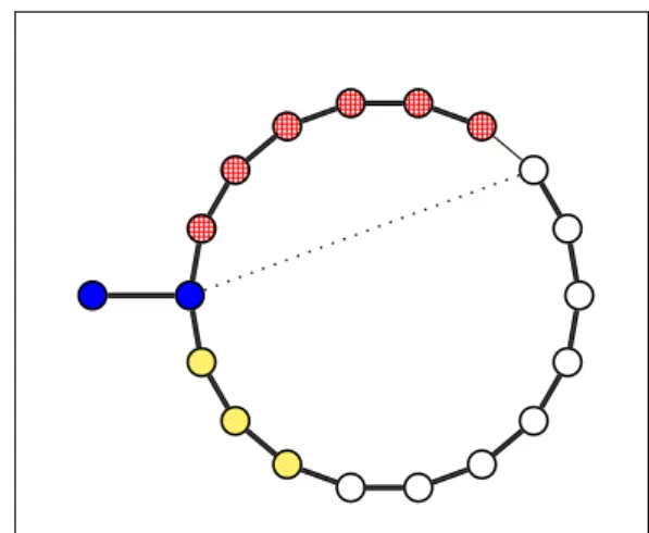
Proof. Suppose by way of contradiction that𝒜 is a protocol for counting which requires at most 𝑡(𝑛) rounds in 1-interval connected graphs of size 𝑛. Let 𝑛′ = max {𝑡(𝑛) + 1, 𝑛 + 1}. We will
show that the protocol cannot distinguish a line of length𝑛 from a line of length 𝑛′.
Given a sequence𝐴 = 𝑎1∘. . . ∘𝑎𝑚, letshift(𝐴, 𝑟) denote the cyclic left-shift of 𝐴 in which the
first𝑟 symbols (𝑟 ≥ 0) are removed from the beginning of the sequence and appended to the end.
Consider an execution in a dynamic line of length𝑛′, where the line in round𝑟 is composed of two
adjacent sections𝐴 ∘ 𝐵𝑟, where𝐴 = 0 ∘ . . . ∘ (𝑛 − 1) remains static throughout the execution, and
𝐵(𝑟) = shift(𝑛 ∘. . .∘(𝑛′− 1), 𝑟) is left-shifted by one in every round. The computation is initiated
by node0 and all other nodes are initially asleep. We claim that the execution of the protocol in
the dynamic graph𝐺 = 𝐴 ∘ 𝐵(𝑟) is indistinguishable in the eyes of nodes 0, . . . , 𝑛 − 1 from an
execution of the protocol in the static line of length𝑛 (that is, the network comprising section 𝐴
alone). This is proven by induction on the round number, using the fact that throughout rounds
0, . . . , 𝑡(𝑛) − 1 none of the nodes in section 𝐴 ever receives a message from a node in section 𝐵:
although one node in section𝐵 is awakened in every round, this node is immediately removed and
attached at the end of section𝐵, where it cannot communicate with the nodes in section 𝐴. Thus,
the protocol cannot distinguish the dynamic graph𝐴 from the dynamic graph 𝐴 ∘ 𝐵(𝑟), and it
If 2-interval connectivity is assumed, it becomes possible to solve gossip under asynchronous start. We begin by defining a version of the𝑘-committee and 𝑘-verification problems that explicitly
address sleeping nodes.
𝒌-Commitee with Wakeup. In the modified 𝑘-committee problem we require, as before, that no
committee have more than𝑘 nodes. Sleeping nodes are not counted as belonging to any committee.
In addition, if𝑘 ≥ 𝑛, we require all nodes to be awake and to be in the same committee.
𝒌-Verification with Wakeup. In the modified 𝑘-verification problem, all awake nodes must
eventually output 1 iff𝑘 ≥ 𝑛. Sleeping nodes do not have to output anything. (Nodes that are
awakened during the execution are counted as awake and must output a correct value; however, there is no requirement for the algorithm to wake up all the nodes.)
5.5.1 𝒌-Verification with Wakeup
We modify the𝑘-verification protocol as follows. First, each node that is awake at the beginning of
the computation maintains a round counter𝑐 which is initialized to 0 and incremented after every
round. Each message sent by the protocol carries the round counter of the sender, as well as a tag indicating that it is a𝑘-verification protocol message (so that sleeping nodes can tell which protocol
they need to join).
As before, each node𝑢 has a variable 𝑥𝑢 which is initially set to its committee ID. In every
round node𝑢 broadcasts the message ⟨𝑘-ver, 𝑐𝑢, 𝑥𝑢⟩. If 𝑢 hears a different committee ID or the
special value⊥, it sets 𝑥𝑢 ← ⊥; if it hears a round counter greater than its own, it adopts the greater
value as its own round counter. When a node𝑢 is awakened by receiving a message carrying the 𝑘-ver tag, it sets 𝑥𝑢 ← ⊥ and adopts the round counter from the message (if there is more than one
message, it uses the largest one).
All awake nodes execute the protocol until their round counter reaches2𝑘. At that point they