A distributed and iterative method for square root filtering in space-time estimation

LIDS-P-222 6

A Distributed and Iterative Method for Square Root Filtering in

Space-Time Estimation*

Toshio M. Chint

William C. Karl$

Alan S. Willsky§

January 19, 1994

Abstract

We describe a distribute, and iterative approach to perform the unitary transformations in the square root information filter imple nentation of the Kalman filter, providing an alternative to the common QR factorization-based approach s. The new approach is useful in approximate computation of filtered estimates for temporally-evolving rando:n fields defined by local interactions and observations. Using several examples motivated by computer vision applications, we demonstrate that near-optimal estimates can be computed for problems of practical importance using only a small number of iterations, which can be performed in a finely parallel manner over the spatial domain of the random field.

'This research was supported in part by the Air Force Office of Scientific Research under Grant F49620-92-J-002, the Office of Naval Research under Grants N00014-91-J-1120 and N00014-91-J-1004, and the Army Research Office under Grant DAAL03-92-G-0115. Address for correspondence: Toshio Chin, RSMAS-MPO, 4600 Rickenbacker Causeway, Miami, FL 33149. t with the Rosenstiel School of Marine and Atmospheric Science, University of Miami, and formally with the Laboratory for Information and Decision Systems, M.I.T.

$with the Laboratory for Information and Decision Systems, M.I.T.

with the Laboratory for Information and Decision Systems and the Department of Electrical Engineering and Computer Science, M.I.T.

1

Introduction

We describe a highly parallel approach to the square root information (SRI) filter (Bierman, 1977) imple-mentation of the Kalman filter. Our motivation for developing this method comes from the field of image sequence processing and computer vision. In applications such as the estimation of motion and reconstruc-tion of surfaces in image sequences we are faced with the problem of estimating an entire spatial field at each point in time. For example, in computation of "optical flow" (Horn and Schunck, 1981) a two-dimensional apparent velocity vector is to be estimated in each pixel; thus, for a 256 x 256 image we are faced with updat-ing more than 100,000 (2 x 256 x 256) variables over time. While image processupdat-ing has provided the original motivation for our work, problems of this scale potentially arise in any distributed parameter estimation or control application in which estimates of spatially-distributed processes are to be computed and tracked.

For problems of such large dimensions, a straightforward implementation of recursive estimation equa-tions such as the Kalman filter is prohibitively expensive. In particular, the calculation, propagation, and storage of the error covariance and Kalman gain matrices are often impossible. Indeed in many applica-tions, including the estimation of optical flow and surface reconstruction, the measurement matrix can be data-dependent, requiring on-line calculation of the filter covariance and gain - an even more unreasonable demand. Consequently, there are compelling reasons to develop alternate, computationally efficient, and hopefully near-optimal approximations to the Kalman filtering equations.

The key to our approach to this approximation problem is that the inverse of the square root of a covariance matrix has a natural interpretation as a model for a random phenomenon. As an illustration,

consider a standard discrete state-space model

x(s) = a(s - 1) +w(s), (1)

X(0) = Xo (2)

where :0 is a zero-mean random variable and w(s), 1 < s < n, is zero-mean white noise independent of azo. If we let x be the vector constructed by stacking x(0) through :(n) and let w be the vector consisting of

zo, w(1),..., w(n), then our model becomes

Mx = w (3)

where M is a lower bidiagonal matrix capturing both the dynamic equations (1) and initial condition (2). From (3) we see that the covariance P of x is given by

P = M-lQM- T (4)

where Q is the diagonal covariance matrix of w. Thus, except for the simple scaling implied by the presence of Q on the right-hand side of (4), the matrix M is the inverse of the square root of the covariance of x.

Similarly, if we have a 2-D random field f(sl, s2) described by the 2-D difference equation

aof(Sl, S2) + alf(sl + 1, S2) + a2f(sl, S2 + 1) + a3f(Sl -1, S2) + a4f(sl, 2 - 1) = W(S 1, S2), (5)

together with appropriate (e.g. Dirichlet) boundary conditions, we can again collect the variables f(sI, s2) into a vector x as well as the variables w(s1, s2) and the boundary conditions into a vector w, so that x and w are once again related as in (3). The associated matrix M, while not being lower bi-diagonal, is extremely sparse and, of course, spatially local.

Having such sparse structures in the inverse of the square root of a covariance matrix has important consequences for the interpretation and computation of the SRI filtering algorithm. Consider the Kalman filtering problem for the discrete dynamic system

x(t) = A(t)x(t - 1) +w(t) (6)

y(t) = C(t)x(t) + v(t) (7)

where w(t) and v(t) are independent Gaussian white noise processes with covariances Q(t) and R(t), re-spectively. Let x(t) be the filtered estimate, i.e., the conditional mean x(t) =_ E[x(t) I y(r), r < t], and x(t) be the associated estimation error with covariance P(t). Define the SRI matrix r(t) to be the inverse of a square root of P(t), i.e. a square matrix such that rT(t)r(t) = P-'(t). The SRI filtering algorithm performs recursive propagation of r(t) and of z(t) - r(t)g(t). We will refer to ( z(t), r(t) ) as the SRI pair, in contrast to the conditional mean and covariance pair ( (t), P(t) ).

If we wish to compute the optimal estimate x(t) given the SRI pair, we need to solve

r(t) x(t) = z(t) . (8)

For the problems motivating this work, explicit inversion of r(t) and even the exact calculation and storage of r(t) are prohibitively complex. However, if r(t), or more precisely an adequate approximation of r(t), were sparse and banded, then (8) could be solved efficiently using various methods of numerical linear algebra, such as successive overrelaxation, multigrid, etc. The main computational issue in the Kalman filtering problem is, therefore, how to time-recursively compute the elements of the matrix r(t) or its sparse approximation efficiently. A spatially distributed method to perform this computation is presented in this paper. Note that, as we have observed, r(t) provides us with what can be viewed as either a whitening filter or a model for the estimation error x(t), i.e.,

r(t) x(t) = 6(t)

(9)

where 6(t) is zero-mean with identity covariance. Computation of r(t), then, corresponds to the specification

of a spatial' model for the components of the error x(t) for each t. Thus, specifying a sparse approximation to r(t) corresponds precisely to reduced-order spatial modeling of the error field x(t).

In this paper we present an iterative, highly parallelizable algorithm for the implementation of the optimal SRI filter. In addition to showing that this alternative to the previously-developed SRI filter algorithms does indeed converge in general, we also demonstrate that the highly parallel structure of our iterative procedure

naturally leads to surprisingly effective and computationally efficient algorithms for suboptimal estimation in situations in which the exact computation and storage of r(t) is not feasible. In particular, we show a reduced-order filtering technique that constrains the SRI matrix r(t) to be manageably sparse at all times. We focus most of our attention on the issue of how to propagate this sparsely approximated SRI matrix, denoted as r,(t), and its accompanying vector za(t)

z

ra(t)R(t) efficiently over time.

2

Model Based Approximation

To provide a more precise picture of the type of approximation we seek, let us consider a general space-time estimation problem that might arise in distributed parameter estimation problems and image processing applications. In particular, we wish to estimate an unknown random field f(s, t) over a discrete space s E ZK and time t E Z, where Z is the set of integers, based on the dynamic system formulation (6),(7). For this work we focus on the case where the space-time dynamics are specified by a set of local interactions (e.g. a set of partial differential equations) and the observations are correspondingly local (e.g. point or weighted-sum observations). The state vector x(t) is defined to be a temporal slice of the random field sampled at time t and over the entire spatial domain consisting of n spatial sites. Equation (6) represents the temporal dynamics of this spatio-temporal field (e.g., a spatially and temporally discretized version of the partial differential equation for the field), and (7) specifies the local measurements of the field at some or all of the points in the spatial domain. In general the spatial domain is a K-dimensional rectangular grid, and the elements z(i, t), 1 < i < n, of the vector x(t) are the random variables f(s, t) ordered lexicographically according to the spatial coordinates s = (sl, 2, ... , sK). Specifically, let sk = 1, 2, ... , nk for k = 1, 2,..., K; then, we let x(i, t) f(s, t) where the index i and grid coordinates s have one-to-one correspondence

K k-1

i =1S + Z(sk- 1)

J

nj. (10)

k=2 j=1

As we will see, for the cases of interest in this work (dominated by local interactions and observations), this lexicographical ordering of the spatial sites leads the key matrices - including A(t), C(t), and

r(t)

-to adopt predominantly diagonally banded structures. Organizing the matrix elements by their diagonal bands allows us to make a coherent presentation of our spatially distributed filtering algorithm, as we switch I It is important to emphasize that this perspective interprets r(t) as a model among the components of x(t) at each instant

back and forth between matrix row position indexed by i and the spatial domain spanned by s. Note that

n = dim(x) = 1-k=l nk, implying a large dimension of the state vector and SRI pair. For example, filtering

of a 512 x 512 image sequence requires us to contend with vectors x(t) and z(t) of about quarter million elements each and a matrix r(t) of square that dimension. For simplicity, let us assume that f(s, t) is scalar-valued for now; we discuss the cases where f(s, t) is a vector field in Section 4.2.4.

Estimates of the random field can be obtained, in principle, by Kalman filtering or smoothing based on (6),(7). Compared with standard Kalman filtering algorithms, square root algorithms are known for their superior numerical properties (Bierman, 1977, Kaminski et al., 1971), especially desirable in applications in which the space-time filters are the hard-wired, high-speed "front-ends" of complex control systems (e.g. Masaki, 1992). With the typically large dimension n of the spatial domain (and of the state vector), however, exact recursion of the SRI pair, costing O(n3) flops for each t, is computationally infeasible in practice. To

address this computationa problem, it is useful to realize that each time-step of the Kalman filter or its SRI implementation can be viewed explicitly as a purely spatial processing problem. Specifically, the one-step-ahead prediction step in the filter corresponds to the estimation of a predicted field based on the estimate at the current time, together with a computation of a spatial model for the errors in this predicted estimate, as captured by the error covariance or SRI matrix. Similarly, the update step involves both the spatial processing of the new observations to update the predicted field together with the updating of the corresponding spatial model for the errors in this updated field estimate.

Note that the solution of (8) can also be viewed as the solution of a spatial processing problem. In particular, let yii be the elements of the matrix r(t). Then, the ith row of the matrix equation (8) is

-'E

= ij (i, = t) (11)

j=l

where z(i, t) and 2(i, t) are the ith elements of the vectors z(t) and x(t), respectively, and where the index i is related to the spatial coordinates s via (10). Also, from (9) we see that the spatial model for the estimation error x(t) satisfies an equation exactly as in (11) but with 2(j,t) replaced by i(j,t) and z(i,t) replaced by the unit variance spatial white noise process 6(i, t).

The domain of the summation in (11) is over all the spatial sites, implying that the computation of x(t) from z(t) is a demanding task and that the white-noise-driven spatial model for the estimation error x(t) has an order equal to the extent of the entire spatial domain of interest. This insight naturally suggests the idea of seeking a reduced-order, spatially local, approximate model in place of the exact r(t). Specifically, in such a model the support of the summation in (11) is reduced as

EY yij (j,t) = z(i, t) (12)

where A/i is a small set of the indices for spatial sites local to the site i. The cardinality of the set A.i roughly

determines the order of the model, which in our applications will generally be taken to be 0(1) rather than

O(n). For example, in a "nearest-neighbor" (Levy et al., 1990) approximation on a 2-D spatial domain (K = 2) as in (5), for each i, XVi is the index set corresponding to the set of coordinates

{(sl,s ₂), (sl + 1, s₂), (s - 1, s2), (sl, 2 + 1), (s, s2 - 1)} (13)

where (sl, s2) are the coordinates of site i. This reduced-order modeling framework is clearly related to the idea of specifying an approximate local Markov random field model (Wong, 1968) for a given spatial process. For this reason we borrow from Markov random field terminology and refer to the set Afi as a neighborhood. Without much loss of generality, we consider a spatially homogeneous neighborhood parameterited by a single integer v, which we call the radius of the neighborhood, as follows:

Definition 1 (neighborhood) Let ju be the site indez corresponding to the spatial coordinates u, and si

be the spatial coordinates corresponding to the site indez i. Then, for a given non-negative integer v, let the

neighborhood

KAi

be the set of site indices such that

Ai- {ju : lu - si L< } (14)

where Lu - sl denotes the "1-norm" or "Manhattan distance", i.e., -- 1 Iuk -ski.

Thus, by specifying v (hence the set of neighborhoods {Afi, i E [1, n]}), we can approximate (8) based on the reduced-order approximation (12) as

ra(t)xa(t) = za(t). (15)

In another words, r,(t) is obtained from r(t) by windowing, or by setting 7ij = 0 for j i Afi,Vi. Note that the vector z(t) has been approximated along with r(t) because, as we will see in the next section, propagation of z(t) is coupled to that of r(t).

Truncating the domain of summation as in (12) does not mean ignoring statistical correlations between process elements over a long distance. Rather, we have constrained the order of the model used to cap-ture these correlations, which certainly can extend over the entire spatial domain even when the spatial interactions are strictly local (Habibi, 1972).

In the next section we will describe the iterative SRI filter algorithm. We present a result showing that if carried to completion this algorithm does indeed converge to the optimal SRI filter. We then describe in Section 4 a constrained version of the algorithm which stops far short of "completion" and in fact typically involves only a small number of iterations. For problems such as the space-time estimation applications we have mentioned, our SRI filter algorithm has a spatially distributed computational structure desirable for processing variables supported over a large spatial domain and, in particular, for carrying out the com-putations necessary for propagation of the approximate SRI pair ( z(t), r1a(t) ) in time. Various existing

implementations of the SRI filter algorithm, particularly those based on the QR factorization (Golub and van Loan, 1989), including systolic array algorithms (McWhirter, 1983, Kung and Hwang, 1991), do not feature such fine-grain parallelizability. We explicitly address the estimation of space-time processes and illustrate the effectiveness of our algorithm with several examples. Using the approximate SRI filter algo-rithm, near-optimal filtered estimates are obtained experimentally with a computational cost per time step that is O(n), reduced significantly from the theoretical cost of O(n3), which is prohibitively large for the

typically large values of n encountered in distributed parameter estimation and computer vision problems. Furthermore, if the approximate filter is implemented in parallel, a throughput cost 0(1) per time step can be achieved for the propagation of ( z,(t), r,(t) ).

3

Iterative Square Root Filtering

In this section we describe a general iterative algorithm for the implementation of the SRI filter. This general algorithm will be used in Section 4 as the basis for development of an efficient near-optimal filter for space-time estimation problems. To start, we review the steps of SRI filtering for the system (6),(7). In the SRI context the process and measurement noise covariances Q(t) and R(t) are typically specified directly in terms of their respective inverse square roots, W(t) and V(t) (so that WT(t)W(t) = Q-'(t) and

VT(t)V(t) = R-1(t)). Since the central operations in SRI filtering involve unitary transformations, we will

adopt a shorthand notation for such an operation; the expression E1 -- + 12 denotes that the matrix 12 is obtained by applying a unitary transformation to the matrix El. Also, let the dimension of the observation vector y(t) in (7) be m, which is usually O(n). The computation of the SRI pair at time t from the pair at time (t - 1) involves two steps: the prediction step, in which r(t - 1) and z(t - 1) are predicted ahead to time t, and the update step, in which the new measurement is used in determining r(t) and z(t). The prediction from time (t - 1) to time t through the dynamic equation (6) is accomplished by the following unitary transformation, which nulls the lower-left n x n block in a 2n x (2n + 1) matrix:

r(t - 1) o z(t- 1) *nxn *nxn *nx1

-W(t)A(t) W(t)

0

L

r (t)

(t)

16)

The lower-right n x (n+ 1) block of the transformed matrix yields the predicted SRI pair ( (t), r(t) ). Hlere, *'s denote generically non-zero blocks and their subscripts indicate the block sizes. The SRI pair ( _(t), 1r(t) ) is then updated by the observation equation (7) using another unitary transformation:

r(t) z-(t)

l'

_

[

l

* 1

z(t)

(17)

V(t)C(t)

V(t)y(t)

0

*mx

in which the lower-left m x n block is nulled. The upper n rows of the transformed matrix yield the updated SRI pair ( z(t), r(t) ). The filtered estimate x(t) is then obtained from this updated SRI-pair as the solution of

(8). Each of the stages (16),(17),(8) costs O(n3) flops in general, and these three stages are the computational

bottlenecks of an SRI filter algorithm. See (Bierman, 1977, Kaminski et al., 1971) for more details.

3.1

Unitary transformation by QR factorization

The unitary transformations (16) and (17) are commonly performed with QR factorizations which null the selected matrix elements sequentially, in essence by a repeated application of Givens rotations2 (Golub and van Loan, 1989). Let ti's and bi's be the elements of two full rows, respectively, of the left hand side matrix in (16) or (17). Givens rotation 9 operates on two such rows so that a specific element (e.g., bo) is nulled:

cos 09 -sin p*-- t-l to tl -t'1 to t ...

sin8 cos

L.

b_ b0 bl -

J

... b 1 0 b

J

where 9 is evaluated based on to and bo; for convenience we say "the rotation 6 is defined by {to, bo}." Since the purpose of the two unitary transformation steps is to null out the lower left block, every Givens rotation involved in these steps is "defined" by a pair of elements in the left-most column of the matrix blocks. Let the left-most column of blocks in (16) and (17) be denoted as

i.e., the matrix (t), while E D plays the roles represents the matrices of t- 1) and (18) i.e., the matrix D plays the roles of r(t - 1) and f(t), while E represents the matrices -VW(t)A(t) and

V(t)C(t), in each of the respective steps. The unitary transformation that nulls the block E in each case accomplishes the propagation of the SRI pair as specified in (16) and (17).

In a QR factorization-based implementation of the unitary transformation steps, the elements are nulled sequentially. Below, we display the matrix (18) when n = 4 (for convenience we let the block E to be square). In essence, the QR factorization nulls the elements marked by the numbers 1 through 22 in numeric order,

2

A typical implementation of the QR factorization involves a serial application of Householder reflections which themselves can be considered as series of Givens rotations.

yielding an upper triangular matrix as the output: dl * * * * * 7 d2 * * * * 6 13 d3 * * 5 12 18 d4 * D --- -. ... (19) 4 11 17 22 3 10 16 21 2 9 15 20 1 8 14 19

The elements along the mein diagonal of block D, marked by dl d2d3d4, are always involved in defining

the Givens rotations. The .R factorization is accomplished by a sequence of Givens rotations defined by

{dl, 1},{dl,2},...,{dl, 7}, {d2, 8}, {d2,9},..., etc.

The QR factorization con Dletes each of the unitary transformations in a finite number of Givens rotations and allows pipelined computation on systolic arrays (McWhirter, 1983, Kung and Hwang, 1991). In terms of space-time estimation, however, such an approach is computationally unattractive and often infeasible, because of the structure of the computations required in standard QR factorization algorithms. In particular, the strictly ordered nulling procedure inherent in QR methods, when applied to space-time processes, yields a computational structure that is spatially sequential, implying that the variables at certain spatial sites cannot be processed until processing at every other site is completed. Such an approach has obvious disadvantages for problems defined on spatial grids of even moderate size. Moreover, in the QR factorization-based algorithms the SRI matrices are triangular matrices so that the inversion in (8) is usually accomplished by back-substitution (Golub and van Loan, 1989), another spatially sequential procedure. For space-time problems, it is usually preferable to seek algorithms with spatially local and highly parallelizable structure. For example, if the matrix

r(t)

is tridiagonal (or block tridiagonal with tridiagonal blocks, as it is for nearest-neighbor models over 2-D spatial domains), (8) can often be efficiently solved using an iterative method, such as successive over-relaxation (SOR) (Golub and van Loan, 1989) or multigrid (Terzopoulos, 1986) methods, which are highly parallelizable and spatially local with comparatively modest memory requirements. In general such methods are effective and computationally efficient for inversion of a sparse set of equations. This observation motivates the objective of Section 4 of obtaining a sparse approximation to (16),(17),(8) with a resulting sparse approximation to the SRI matrix, namely ra(t). Of course, for this objective to make sense, we must also use a spatially local and highly parallel method to calculate our approximate SRI matrix, which we develop below.

3.2 An iterative unitary transformation

As we have indicated, a standard approach to the computations in (16),(17) uses a sequential application of Givens rotations to null out the desired elements one at a time. The basic idea behind our distributed and parallel algorithm is to apply a number of these rotations simultaneously. As we will see, an element that has been nulled at one step in this approach may become non-zero subsequently, in contrast to the standard QR algorithm. However, our algorithm has the property that the repeated iterative application of this procedure does in fact asymptotically null the desired block. To illustrate the basic idea, consider an alternative way to null the submatrix E in matrix (18) - use the main diagonal of the D to null every diagonal band in E in sequence. The elements in a diagonal band in E can be nulled simultaneously, as the Givens rotations are applied to disjoint pairs of rows of matrix (18). This method is iterative: every diagonal band in E is

repeatedly nulled, because in general nulling of a band transforms a previously nulled band elsewhere back to

a non-zero band (whose elements are usually smaller in magnitudes than before). For the n = 4 case treated in (19), d * * * * d * * * * d * * * * d

[

E]

_

__ _

__ ,(20)

1 2 4 6 3 1 2 4 5 3 1 2 7 5 3 1

the main diagonal marked by d's in the upper block D nulls the diagonal bands numbered by 1 through 7 in the lower block E in sequence. In general the ordering of the bands to be nulled can be arbitrary. Let us define a sweep to be a single round of nullings in which every element in E is nulled exactly once, e.g., the seven band-nullings in (20). As elaborated below, the entire submatrix E can be nulled by repeating the sweep.

To describe our iterative unitary transformation algorithm more formally, let D be an arbitrary n x n matrix whose elements are denoted as dij, and let E be a p x n matrix whose elements are eij. WVe again consider the generic unitary transformation problem of nulling the lower submatrix E in the matrix (18) by application of a series of Givens rotations.

Definition 2 (sweep) Consider, for each of the pn elements eij of the submatriz E, a Givens rotation

defined by {djj, eij) and applied to the the jth row of D and it h row of E to null the element eij . For matriz

In a sweep, the elements in E can be nulled in any order as long as each element is nulled once. Also, note that the diagonal elements dij are the only elements of submatrix D that participate to define the Givens rotations. While we have indicated that a sweep involves sequential Givens rotations, highly parallel implementations are possible by exploiting the fact that the Givens rotations can be applied to disjoint sets of rows concurrently, since the actions of these rotations do not interfere with each other. Specifically, the set of elements {eij : i - j = constant} forms a diagonal band of the submatrix E, and the elements in such a band can be nulled simultaneously as exemplified in (20). This band-wise implementation of sweep, referred to as a band-sweep, plays the key role in the SRI filtering algorithms presented in this paper.

Definition 3 (band-sweep) A band-sweep is a special case of a sweep, such that the elements eii in a

diagonal band {eij : i - j = constant} of submatriz E are nulled concurrently.

One price we pay for this parallelism is that elements of E that are nulled at one point in a sweep may be made nonzero later in the sweep. That is, after the element eii is nulled, a subsequent Givens rotation applied on the ith row of E can turn eij non-zero. The following result (proved in Appendix), however, assures that asymptotically the entire submatrix E is nulled.

Theorem 1 An iterative application of sweeps to the matrix (18) nulls the block E in the limit.

In particular, iterations of the parallelizable band-sweeps are guaranteed to converge and are applicable to optimal recursion of the SRI pair in a generic SRI filtering algorithm.

Algorithm 1 (Parallel Recursion of the SRI Pair) In the unitary transformation steps (16) and (17),

use iterations of band-sweep to null the respective lower-left submatrices.

Note that band-sweeps can achieve a still higher level of concurrency by defining the diagonal band cyclically. For example, in (20) all the lower block elements labeled 2 and 7 can be considered to be a single cyclic diagonal band which can be nulled simultaneously, as are those labeled 3 and 6 as well as 4 and 5. Such a cyclical computational structure might be useful for a space-time estimation problem with a torroidal spatial domain.

In general, the number of iterations required for convergence of the unitary transformation algorithm depends on the specific values and structures of the constituent matrix blocks in (16) and (17). In SRI filters arising in space-time estimation problems and the approximate filters based on them, the structure inherent in the matrices of such problems allows the development of nulling strategies that exploit both the natural and imposed sparseness and bandedness of the matrix blocks. The end result is an extremely efficient unitary transformation procedure which requires only 3 or 4 sweeps for an adequate accuracy as demonstrated later with numerical examples. For the rest of the paper we concentrate our discussion on such space-time filtering problems.

4

Space-Time Estimation

The iterative unitary transformation method is especially suitable for the reduced-order approximation of the space-time estimation problems described in Section 2, as the distributed nature of the algorithm can take advantage of the sparsely banded structure of these estimation problems. The dynamics of such space-time random fields are typically specified by a set of local interactions among the components of the field, usually expressed in terms of a set of stochastic partial difference equations. The spatial locality of these interactions and the corresponding observations is then reflected in sparsely banded structures of the matrices A(t), W(t), C(t), and V(t) in the system equations (6),(7). See Section 4.2 for illustrations of problems

with this type of structure.

Let us consider the SRI filter (16),(17),(8) in the context of such a space-time estimation problem. As discussed previously, the computational cost of O(nr3

) associated with exact implementation of each of these

steps is impossibly large for typical values of n. We thus seek an approximate filtering algorithm. First, the SRI matrix

r(t) is sparsely approximated as

ra(t)

based on the reduced-order model approximation (12). As discussed previously, this approximation makes (8), or more precisely (15), a manageably sparse equation that can be solved efficiently by iterative inversion methods whose throughput cost can be as low as 0(1) for the typically large values of n encountered in practice (Terzopoulos, 1986). For spatial estimation problems of practical interest, however, we cannot calculate or store the matrices r(t) or r(t) and thus cannot directly generate the approximations to these matrices by simply windowing them. What we desire, then, is an algorithm that directly and efficiently propagates ra(t) itself in time.

4.1

A reduced-order filtering algorithm

Suppose that at some point in time we do have a sparse approximation to r(t) or r(t). In this case, notice that all the matrix blocks involved in the left hand sides of (16) or (17) also have sparsely banded structures. This insight leads to the idea of incorporating another level of approximation into the SRI filter algorithm, beyond that associated with (12). In particular, the sparseness and special structure of the matrix blocks in (16),(17) are exploited to perform the associated iterative unitary transformations in an approximate and highly efficient manner, producing sparsely banded approximations to r(t) and r(t) directly and recursively in time. The basic idea behind this second level of approximation is to use the band-sweep algorithm described in association with Algorithm 1, but only to make partial sweeps which are matched to and consistent with the desired banded structure of the matrices that are to be maintained in the approximate filter. Specifically, since the matrix blocks at each stage of the algorithm are sparsely banded to begin with, we may be able to efficiently constrain each of these blocks to have a certain sparsely banded structure throughout the duration of the iterations and thus decrease overall throughput cost. That is, we limit the extent of each band-sweep to a finite and typically small number of bands, thus reducing dramatically the number of elements which are to be nulled in each cycle. In the space-time problems we have examined and will illustrate in Section 4.2,

the computational cost of each iteration of the approximated band-sweep is usually 0(1) per spatial site as a result.

Our approximation of the full SRI filtering algorithm is characterized by two types of neighborhood sets, which are used to constrain the structures of both the matrix blocks and the algorithm itself. The first type of neighborhood corresponds to the spatial model we wish to use to describe the statistics of the error field; it corresponds to the set of neighborhoods XAi which specify the desired order of the approximate error field models in (12). Therefore, these neighborhoods serve to focus modeling resources. These neighborhoods in turn imply that only certain elements of ra(t) are allowed to be nonzero, resulting in a sparsely banded approximation to the SRI matrix. Thus, we can identify the neighborhood set {Ahi, i E [1, n]} as a con-straint on matrix structure. The second type of neighborhoods used by our approximate filtering algorithm are strongly linked to the first type XAi but are basically algorithmic in nature. Specifically, consider the neighborhoods Mi specifiet' by the radius jt (cf. Definition 1) as

Mi = {ju : lu-sit _</}. (21)

They correspond to the redu :ed subset of bands of the band-sweep algorithm which will be nulled at each stage of the approximate algorithm, and thus reflects a focusing of computational resources. This viewpoint provides us with a rational way of understanding how our computational and modeling resources are linked. Naturally, the computational resource must be at least as large as the support of the desired model. That is, we must have Mi

2D

A, or A k v, for time-recursion of the reduced-order model. Experiments showing

the effects of varying choices of A and v will be presented in Section 4.2.

Definition 4 (partial band-sweep) A partial band-sweep is an approzimate band-sweep in which all

the participating matriz blocks are windowed by the neighborhood set {AMi. That is, in each submatriz, the

(i, j)th elements for j q Mi are treated as zeroes throughout the band-sweep iterations.

In the spirit of our generic notation "'A -' 12" for the exact unitary transformation, we denote an approximate unitary transformation performed with this partial band-sweep operation by the expression

1 M; 12. In general a matrix block windowed by the neighborhood set {Mi} has only O(;K) diagonal

bands. In a partial band-sweep, only the elements in these diagonal bands ever participate in computation and need to be stored, the rest being treated as being identically zero. Thus, for a small jt, performing such

a partial band-sweep leads to a high throughput rate when implemented in parallel. With this motivation we have the following algorithm:

Algorithm 2 (Reduced-order Space-time SRI Filter) Let (z_(to), ra(to)) be a given initial reduced-order approzimated SRI pair. Specify the radii ja and v, such that g > v, to determine the neighborhood

sets {Mi} and

{.fi},

respectively, hence defining the extent of the partial sweep and subsequent windowing

operation. Also, specify the number of sweeps to be performed for each unitary transformation step. Repeat the following steps for t = to, (to + 1), (to + 2), .. :

1. Prediction Step.

Iterations of partial band-sweeps are applied to approzimate the unitary transformation of the ezact prediction step (16)

ra(t-

1) 0 z.(t- 1) *nxn nxn *nl

1

(22)

-W(t)A(t) W(t) o0

Jnxn

r (t) a(t)

J

The lower left block en xn on the right hand side denotes a generic small, but non-zero, matriz in this position resulting from use of the approzimate band-sweep-based unitary transformation.

2. Prediction Windowing Step.

The matriz rb(t) on the right hand side of (22) is now further windowed by {fA} to obtain r.(t).

This windowing assures that ra(t) will have the same band structure as ra(t - 1). The approzimate

predicted SRI pair is then given by ( (t), ra(t) ).

3. Update Step.

Iterations of partial band-sweeps are again applied to approzimate the unitary transformation of the ezact update step (17)

ra(t) _ (t) ] MW rb(t) 1_(t)

(23)

V(t)C(t) V(t)y(t) L mxn *ml

Again, the lower left block emxn on the right hand side denotes a generic small, but non-zero, matrix

in this position again resulting from use of the approximate band-sweep-based unitary transformation.

4.

Update Windowing Step.

The matriz rb(t) on the right hand side of (23) is now further windowed by f{i} to obtain

r

1

(t).

Again, this windowing assures that ra(t) will have the same band structure as

r,(t),

thus maintaining

this structure throughout the calculations. The resulting, approzimate updated SRI pair is then given by ( z.(t), ra(t) )

5. Inversion Step.

If needed, the updated estimate xa(t) may be obtained by solving (by an efficient iterative method such

as multigrid and SOR) the sparse and spatially local set of equations ra(t),a(t) = z(t).

In the above algorithm, a fixed number of iterations (of partial band-sweeps) is used in each of the approxi-mate unitary transformation steps. Alternatively, the iterations can be allowed to continue to convergence within a given numerical tolerance level. In all of the space-time estimation problems we have examined, however, only a very small number (i.e., less than 5) of band-sweeps per unitary transformation step are necessary for reasonably accurate approximations. Such estimation problems are discussed below.

4.2 Numerical Results

The main purpose of the numerical examples presented here is to examine accuracy of various approximations, rather than to record the real-time computational speeds. All computations are performed serially on general-purpose workstations by setting the spatial dimension n manageably small.

4.2.1 Partial band-sweep

We first examine the impact of different choices of the neighborhoods on partial band-sweep in a general unitary transformation problem. The approximating parameters in the partial band-sweep algorithm are the size of the neighborhood Mi, which is given by the integer /A, and the number of iterations of the sweeps. Consider a space-time SRI filtering problem defined over a 1-D spatial domain (i.e., K = 1) and a nearest-neighbor reduced-order modeling approximation (i.e., NAi is specified by v = 1). Note that, under the 1-D nearest-neighbor approximation, all the matrix blocks in the unitary transformation steps (16),(17) of the filter are windowed to be tridiagonal. A key unitary transformation problem is to null the lower block E in the matrix (18) as

and to compute the tridiagonally approximated (windowed) matrix Da of the resulting n x n upper submatrix D. The computation of D itself is approximated by partial band-sweeps defined by the neighborhood Mi of various sizes which are in turn specified by the parameter 1 < pu < n - 1.

We conduct a numerical experiment in which the blocks D and E are randomly generated as 25 x 25 tridiagonal matrices. Let D(e, A) denote the block D after the £th iteration of the partial band-sweep specified by the parameter A, and let Da(i, u) be the tridiagonal matrix formed from the tridiagonal part of the matrix D(e, A). Since p = 24 corresponds to the full band-sweep, Da(oo, 24) is the matrix we seek to approximate by the partial sweeps, i.e., Da = Da(oo, 24). For each t = 1, 2,..., 24 we have computed the normalized error

IIDa(e,

1) - Da(OO, 24)11

(24)

IIDa(oo, 24)11 after evaluating the matrix Da(oo, 24) to convergence.

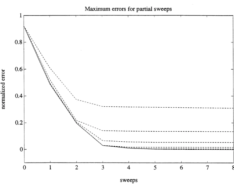
This numerical experiment has been repeated with 10 distinct pairs of D and E. For each of the partial band-sweeps p = 1, 2, 3, 5, 7 and 24, the worst case error, i.e., the maximum values of the error (24' in the 10 tries, is plotted against the number of iterations e in Fig. 1. The figure indicates the speed of convergence, as the error curves level off in roughly 4 iterations. For the full band-sweep (tu = 24) the maximum normalized error after 8 iterations is only 0.0001. The errors for the partial band-sweeps decrease with increasing /z for a small value of 1and then saturate for I > 7. That is, the gain in accuracy diminishes quickly as p increases.

For the partial band-sweep /, = 7, the maximum error after 8 iterations is only 0.0048. These results demonstrate that a partial band-sweep characterized by small neighborhoods can approximate the exact band-sweep accurately (for the purpose of computing windowed transformed matrix blocks) and converge in a very small number of iterations.

4.2.2 Estimation over 1-D space

We now apply the partial band-sweeps examined above to a space-time estimation problem. Consider estimation of a temporally evolving random field f(s, t) over a 1-D space, whose dynamics are governed by a discrete heat equation (Myint-U, 1980) driven by white noise w(s, t) with variance q

f(, t) - f(s, t - 1) =

a[f(s + 1, t) - 2f(s, t) + f(s - 1, t)] + w(s, t),

based on a noisy measurement g(s, t) = f(s, t) + v(s, t) where v(s, t) is a white nosie with variance r. This

estimation problem can be formulated in the state-space format (6),(7) using the following sparsely banded matrices and observation vector

(1-a) a g(1,t) a (1 - 2a) a g(2,t) A(t)= · · , _) = a (1- 2a) a

g(n,t)

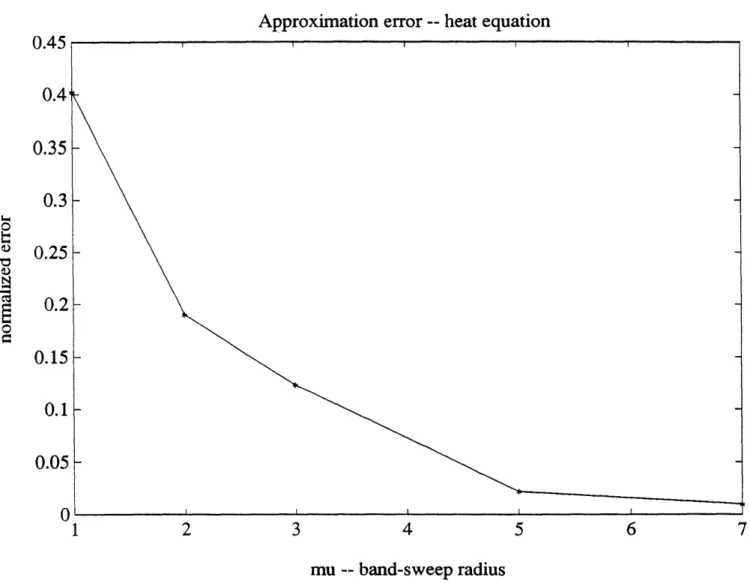
a (1 -a) C(t) = I, W(t) = I, V(t)= I.

A random field and its noisy observations are created using the parameters n = 25, a = 0.4, q = 0.1 and r = 1. The filtered estimates x(t) are computed with the optimal Kalman filter, and they are compared with the approximate estimates x,,(t) computed by Algorithm 2 using the same approximation parameters v and /t's as those examined in Section 4.2.1. In particular, the approximate SRI matrix ra(t) is tridiagonal because Y = 1 specifies the nearest-neighbor reduced-order model. Various approximate estimates corresponding to the partial band-sweeps , = 1, 2, 3, 5, and 7 are computed using only 3 iterations for each unitary transformation in (16),(17). Averaged over 25 repeated experiments, the means of the relative temporal approximation error

Ix~(t)

- _(t)j(

I[_~(t161

~~~~~~~(25)

are computed over the first 10 time frames for each p and plotted in Fig. 2. For A = 7, the average approximation error is less than 1%, exemplifying the accuracy of the proposed approximate SRI filter algorithm with respect to the optimal Kalman filter. Similar sets of experiments conducted with larger v's have not decreased the error significantly, suggesting that the nearest-neighbor approximation is quite adequate for this particular estimation problem.

4.2.3 Estimation over 2-D space

When the spatial domain is multidimensional (K > 1), the matrices A(t), C(t), W(t), V(t), and

ra(t)

have slightly more complex structures than simple banded matrices. Nevertheless, they are still sparsely banded matrices for the cases of interest here, so that Algorithm 2 can offer a high level of parallelism in computation. For example, as we have just seen, the nearest-neighbor approximation v = 1 in the 1-D space case means just to window the SRI matrix r(t) to form the tridiagonal approximation r,(t). When the spatial domain is 2-D, v = 1 leads to

ra(t)

which has a nested block tridiagonal structure, i.e., a block tridiagonal structure in whic h the central blocks themselves are tridiagonal while the first off-diagonal blocks are diagonal. Thus, ra(t) h .s a total of 5 diagonal bands. In general, for a 2-D space estimation problem, the reduced-order modeling a.pproximation specified by a given v yields an approximated SRI matrix with

2v(v+ 1)+1 diagonal bands. We illustrate, with a numerical example, efficiency and accuracy of the proposed

algorithm for filtering over such a spatial domain.

Consider space-time interpolation of f(si, s2, t) based on the smoothness models

f(s1,s₂, t) - f(s ₁,s₂,t- 1) = w(sr,s₂, t) (26) f(s 1,s2,t) - f(s1 - 1, s2, t) = 61(sl, s2,t) (27) f(s1, 2, t)- f(S1,S2 - 1, t) = 62(s1,s 2,t) (28)

and noisy measurements g(sl, 32, t) = f(s1, s2, t) + v( 1, s2, t), where w(s1, s2, t), v(31, 32, t), 61(sl, 32, t), and

62(s1, 83, t) are white noise processes with variances of q, r, 1 and 1, respectively. The models (26),(27),(28)

impose both temporal and spatial smoothness on the reconstructed field, respectively. The problem can be expressed as an estimation problem based on the dynamic system (6),(7) using the matrices and observation vector

A(t) = I, W(t) = I,

yg(t) I 17;

y(t) = 0 C(t) = S , V(t)=

[

(29)

0 S2 I

where the components yg(i, t) of the vector y (t) are the measurements g(si, S2, t) ordered lexicographically as in (10), and S1 and S2 are bidiagonal matrices representing the spatial differencing operations along the

two spatial axes as described in (27) and (28), respectively. An interesting aspect of this formulation is that the temporal smoothness equation (26) is treated as system dynamics while the spatial smoothness equations (27),(28) are relegated to the observation equation (7), a common practice in visual reconstruction (Szeliski, 1989, Chin et al., 1992).

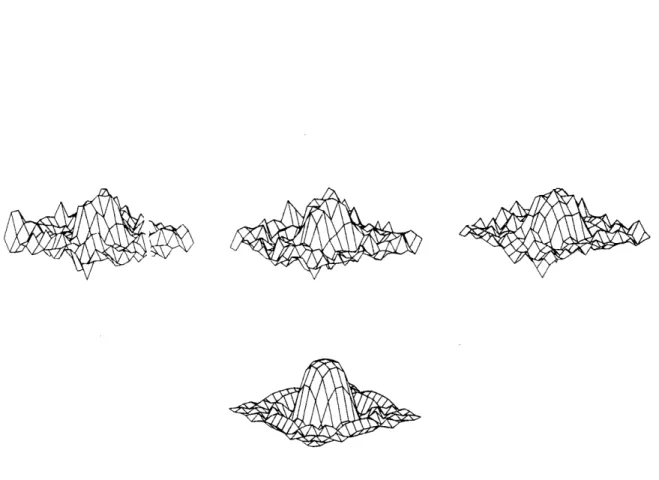
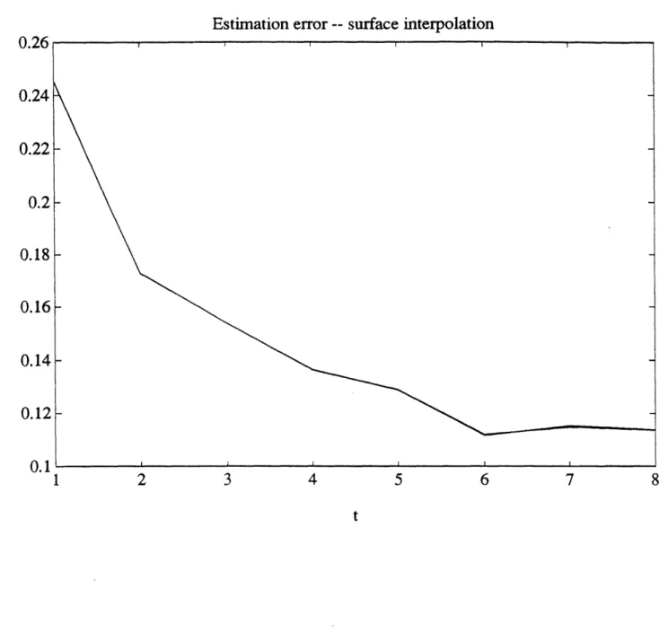
A complete space-time interpolation is possible using two Kalman filters running causally and acausally in time. Here, we examine the causal filter for q = 0.01 and r = 0.25, by comparing the estimates from the optimal Kalman filtering algorithm and Algorithm 2 using various partial band-sweeps. The dimension of the spatial domain is 16 x 16, so that n = 256. Note that the exact optimal estimate can be computed because of the relatively small value of n. For the reduced-order model approximation, we let v = 2. We consider three different partial band-sweeps specified by /s = 2, 3,4. A noise-corrupted surface has been reconstructed using the three approximate SRI filters as well as the optimal filter. Fig. 3 shows the surfaces estimated by the approximate filter using the partial band-sweep specified by t = 4. Normalized estimation errors

IlL4(t) - x(t)I (30)

where x(t) is the true surface, are also plotted in Fig. 4 for all the estimates for the first 8 time frames. These four error curves, which are nearly indistinguishable, show that all three approximate filters have performed virtually identically to the optimal filter for this problem.

4.2.4 Vector field

Finally, let us consider the case where the field variables f(s, t) are vectors. We focus on the specific problem of estimating motion vectors from image sequences and let each f(s, t) be a planar motion vector with two velocity components. Having two (instead of one) unknowns at each spatial site leads to corresponding expansions in the SRI filtering equations; however, the basic form of these equations remains the same. For example, we can simply treat each "element" of the state vector x(t) to be a two-dimensional column vector, while each "element" of such matrices as A(t) and

r(t) is now treated as a 2 x 2 matrix. Algorithm 2

applies to such a vector field estimation problem equally well, after some straightforward adjustments for the increase in dimensionality. In particular, while in the scalar estimation cases each Givens rotation step performs nulling of a single scalar, in the vector case the same step must accomplish complete nulling of a higher dimensional "element". We implement each of these steps using a composite of Givens rotations; if, for example, the "element" consists of 4 scalars, an aggregate of 4 Givens rotations are used to null it. To illustrate how to null one 2 x 2 "element" against another let

d

d1 d2 _ el e2

and consider using a unitary operation to null e against d in the matrix

di d2

Kd1

d3 d4

Le e_l e₂

e₃ e₄

This task can be accomplished by a two-step process: First use d to null the first row [el e2] of e; then, use

d again to null the second row [e₃ e₄]. Each of these steps can be performed by essentially a sequence of two Givens rotations. Specifically, let

[dI d'2 cl 1

::1 [

di d2

dl d' = 1 c2 s2 d3 d4

I el 2e cl -sl - -92 C2 el e2

where ck cos Ok and sk = sin 8k for k = 1, 2. The desired sequence of two rotations 81, 02 can be obtained from the two equations el = 0 and e2 = 0. In practice, it tends to be easier to solve for the ck's and

Sk's directly, aided by the trigonometric identity c2

+ sI = 1. Efficient implementation of the Givens rotations themselves is beyond the scope of this paper. References on this general topic include (Gotze and Schwiegelshohn, 1991, Golub and van Loan, 1989).

Modifying the algorithm as above, we have calculated motion vector fields from an image sequence. The estimation problem is formulated based on the image brightness conservation approach studied by Horn and Schunck (1981) in conjunction with the space-time smoothness models (26),(27),(28) presented in Section 4.2.3. Specifically, by assuming brightness conservation, we can obtain a relationship between the two-dimensional motion vector f(si, s2, t) and spatio-temporal gradients of the image brightness (intensity)

b as

- (s1,s2,t) - [ 0-(s 1,s2, t) -(sl,s 2,t)

]

f(s1 , 2,t), (31)

which we write as g(s1,s₂,t) = h(si,s2,t) f(sl,s2,t) by letting g(sl,s2,t) and h(sl, s2,t) be the scalar on

the left hand side and the first vector on the right hand side of (31), respectively. Because of non-ideal conditions (e.g., measurement noise) in practice, this brightness conservation is not expected to be satisfied exactly at every site. Thus, we assume a more appropriate relationship

g(sl,S₂, t) = h(sl, s₂, t) f(S ₁, S₂, t) + v(S1, S2, t) (32) where the white noise v(sl, s2, t) represents the uncertainty in the brightness conservation with respect to the

particular measurements of the brightness gradients. (The brightness gradients are actually computed from

the measurements of O(sl, s₂, t) by finite differencing.) The observation equation (32) is complemented by the

smoothness models (26),(27),(28) which are necessary for the motion estimation problem to be well-posed (Horn and Schunck, 1981, Chin et al., 1992). The system matrices for (32),(26),(27),(28) are, therefore, essentially vector-field versions of (29), except that C(t) is now a time-varying matrix given by

H(t)

C(t) = S1 (33)

S2

where H(t) is a block-diagonal matrix whose diagonal blocks are h(sl, s2, t). The time-varying nature of the

system necessitates a completely "on-line" implementation of the corresponding Kalman filter.

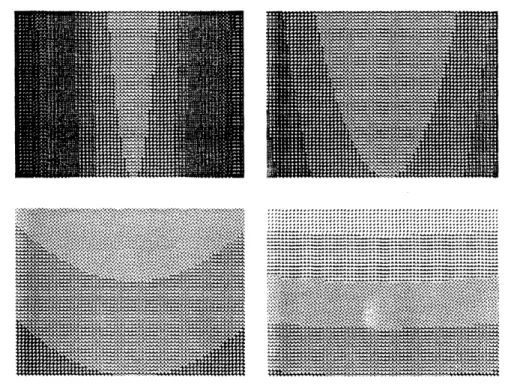
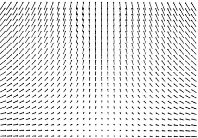
Algorithm 2 has been applied to an image sequence (Fig. 5) describing a simulated fluid flow to yield the estimated flow field shown in Fig. 6, indicating adequate performance of the filtering algorithm. Details of this particular motion estimation problem can be found in (Chin et al., 1992). From a computational perspective, the small image frame size (64 x 48) used in this simulation is still large enough to make an exact, optimal implementation of the Kalman filter impractical. Algorithm 2, however, enables computation of near-optimal estimates. The estimated flow field in Fig. 6 is obtained by using a spatially distributed computational structure over small neighborhoods defined by v = / = 2 and performing only 3 partial band-sweeps per unitary transformation. To invert (15), 100 iterations of the standard Jacobi iterations (Golub and van Loan, 1989) are used.

5

Conclusion

The two main developments of this paper are a novel approach to the unitary transformations in square root filtering, in which the computation can be performed in a finely distributed manner, and an approximation technique for large dimensional space-time SRI filtering problems based on the new unitary transformation. The proposed approximate SRI filter has two levels of approximations characterized by two neighborhood sets. The computational efficiency and near-optimality of the filter have been demonstrated numerically. Systematic selection of the approximation parameters, such as the neighborhood sets and the number of iterations, to approximate an arbitrary space-time problem to a given, desired accuracy is an obvious direction for further research.

Actual parallel hardware implementation of the reduced-order filter (Algorithm 2) also remains as future work. A design based on a layered data mesh, in which the SRI pair and system parameters are stored and band-sweeps are performed, has been explored in (Chin et al., 1993) for specific space-time problems.

The development of this paper was premised on the use of local interaction models (e.g. partial dif-ferential equation models) coupled with local observations of these phenomena. While many space-time estimation problems fit these requirements, there are also non-locally specified problems (e.g., tomographic

measurements used in medicine, geophysics, and oceanography) of practical importance. An interesting and open question is how to efficiently approximate and propagate the SRI pair for such non-local cases.

References

Bierman, G. J. (1977). Factorization Methods for Discrete Sequential Estimation. Academic Press, New York.

Chin, T. M., W. C. Karl, A. J. Mariano, and A. S. Willsky (1993). Square root filtering in time-sequential estimation of random fields. Proceedings of SPIE (Image and Video Processing), 1903, 51-58. Chin, T. M., W. C. Karl, and A. S. Willsky (1992). Sequential filtering for multi-frame visual reconstruction.

Signal Processing, 28, 311-333.

Chin, T. M., W. C. Karl and A. S. Willsky (1992). Sequential optical flow estimation using temporal coherence. accepted for publication in IEEE Transactions on Image Processing.

Golub, G. H., and C. F. 'an Loan (1989). Matrix Computations. The Johns Hopkins University Press, Baltimore, Maryland.

Gotze, J., and U. Schwiege 9hohn (1991). A square root and division free Givens rotation for solving least squares problems on systolic arrays. SIAM J. Sci. Stat. Comput., 12, 800-807.

Habibi, A. (1972). Two-dimensional Bayesian estimate of images. Proceedings of IEEE, 60, 878-883. Horn, B. K. P., and B. G. Schunck (1981). Determining optical flow. Artificial Intelligence, 17, 185-203. Horn, R. A., and C. A. Johnson (1985). Matriz Analysis. Cambridge University Press.

Kaminski, P. G., A. E. Bryson, and S. F. Schmidt (1971). Discrete square root filtering: a survey of current techniques. IEEE Transactions on Automatic Control, AC-16, 727-736.

Kung, S., and J. Hwang (1991). Systolic array designs for Kalman filtering. IEEE Transactions on Signal

Processing, 39, 171-182.

Levy, B. C., M. B. Adams, and A. S. Willsky (1990). Solution and linear estimation of 2-D nearest-neighbor models. Proceedings of IEEE, 78, 627-641.

Masaki, I. (Ed.) (1992). Vision-based Vehicle Guidance. Springer-Verlag, New York.

McWhirter, J. G. (1983). Recursive least-squares minimization using a systolic array. Proc. SPIE Int. Soc.

Opt. Eng., 431, 105-112.

Myint-U, T. (1980). Partial Differential Equations of Mathematical Physics. Elsevier North Holland, New York.

Szeliski, R. (1989). Baysian Modeling of Uncertainty in Low-level Vision. Kluwer Academic Publishers, Norwell, Massachuesetts.

Terzopoulos, D. (1986). Image analysis using multigrid relaxation models. IEEE Transactions on Pattern

Analysis and Machine Intelligence, PAMI-8, 129-139.

Wong, E. (1968). Two-dimensional random fields and representation of images. SIAM J. Appl. Math., 16, 756-770.

Appendix: Proof of Theorem 1

Let D(k) and E(k) be the blocks D and E, respectively, of the matrix (18) after the kth application of the Givens rotation. Also, let dij(k) and eij(k) be the elements of D(k) and E(k), respectively. A unitary transformations like the Givens rotation preserves the 2-norm of the operand vector (Horn and Johnson, 1985); thus, when a Givens rotation is applied to the eth row of D(k) and it h _{row of E(k) we have}

d2j(k + 1) + ei2(k + 1) = d j(k) + e,2j(k), (34)

for j = 1,..., n. Equivalently, the sum of the squares of the elements of the matrix (18) stays constant, i.e.,

c

[-

(,]

(35)

E E(k)

where the subscript F denotes the Frobenius norm (Golub and van Loan, 1989). Let us consider the sequence {d2j(k)}k o for an arbitrary j = 1,..., n. Since

dj3(k) < IID(k)IIF •

[

D(k)

I

Vk,

(35) implies that the sequence is bounded from above by c. Also, in a sweep, an element in the column j of the block E(k) can be nulled only against the element djj(k). That is, when £ = j in (34), the Givens rotation makes e, .(k + 1) zero, or

d2j(k + 1) = d~j(k) + e2j(k). (36)

This implies that the sequence {d2j(k)}k 0 is a non-decreasing sequence for each j. Now, since the sequence

is both upper-bounded and non-decreasing, it must converge. From (36), a necessary condition for the sequence to converge for each j must be limko eij(k) = 0, Vi. This is because every element eij is nulled once in an iteration of sweep, i.e., each element is nulled once every (pn)th application of Givens rotation on

Maximum errors for partial sweeps

0.8

0.6

,

0.4

-

,

,

0.2-

0

1

2

3

4

5

6

7

8

sweeps

Figure 1: The errors in iterative unitary transformations using partial band-sweeps described in Section 4.2.1. The five dotted lines from top to bottom correspond to the partial band-sweeps p = 1, 2, 3, 5 and 7, respec-tively. The solid line is the error for the full band-sweep (i = 24).

Approximation error -- heat equation

0.45

0.4e

0.35

0.3

0.25

-0.2

0.15

-0.1

0.05

-1

2

3

4

5

6

7

mu -- band-sweep radius

Figure 3: Reconstructed surfaces at t = 2, 4, and 6 (top) and the actual surface (bottom).

Estimation error -- surface interpolation

0.26 , ,

0.24

0.22

0.2

i

0.18

-0.16

0.14

0.12

-0.1 ,

1

2

3

4

5

6

7

8

Figure 4: Normalized estimation errors for the first 8 time frames for the optimal filter and approximate filters with tp = 2, 3 and 4. The four error curves are virtually indistinguishable.

-~s~jS | p F S p #Z| a =

-____ 4

z'z7YtY'YzzWzzU....

=| 5 ;. i:: :. :E~~''4WAA~; : i .

Figure 5: Four images from the sequence used in the motion vector computation experiment. Frames 0 and 7 (top row) as well as 14 and 21 (bottom row) are shown.

/

\\\\\\\\\\

,,,,,,,,\\\\\\\\\\\\

7////,,//////,I,,\\I\\\\\\NNN\\N.\ _{//,///I/1, - - I \ \ \\ \\\\\N . \} .-_,,,///?, '..'77//// 1111 _\NN1N\\\\\\\ \\\\\\\\\N\\_{N \\N.N} ,,,,,,,,///,,1/ , \ \\ \ \\\\N\\\ ,,,,////,/,/,,,, ,\\ \ \\\ NNN ,,,,,,,,,,,,,,, t\\ \\\\\\ ,,,,,//////,\\\, ,1 \\\\ N -,, ,,,-, ,...· - = -, -..-. --. .

Figure 6: An optical flow field computed by processing 10 frames of images with the reduced-order SRI filter (left) and the corresponding true flow (right). Every other flow vectors are shown for clarity.