A digital physics method for two phase flow

(1)

A Digital Physics Method for Two Phase Flow

by

David M. Freed

B.S. Double, Nuclear Engineering and Chemical Engineering, University of California at Berkeley (1991)

Submitted to the Department of Nuclear Engineering in partial fulfillment of the requirements for the degree of

Doctor of Philosophy in Nuclear Engineering at the

MASSACHUSETTS INSTITUTE OF TECHNOLOGY May 1997

@

A uthor... .... ... ... ....

Depart e of Nucl r n ering

Certified by... k/ .- Kim olvig Associate Pr essor Thesis Spvisor Accepted by ...

/

/'' / Jeffrey P. Frei'dberg

Professor Reader Accepted by ...

/

/' /Jeffrey P. Frdidberg Chairman, Departmental Committee on Graduate Students

(2)

A Digital Physics Method for Two Phase Flow by

David M. Freed

Submitted to the Department of Nuclear Engineering on April 1, 1997, in partial fulfillment of the

requirements for the degree of Doctor of Philosophy

ABSTRACT

Digital Physics refers to a fully discrete, microdynamical system whose mean be-havior recovers real continuum physics. The purpose of this project is to develop a Digital Physics method by which to model the flow of single-component fluids with a non-ideal-gas equation of state, such as liquids and two-phase mixtures. The new system, called the multiphase system, is built upon the framework of a previously developed Digital Physics system. This original Digital Physics system, the standard system, is used to simulate low Mach number flow of an ideal gas.

Previously, substantial performance improvements (compared to CFD nu-merical solvers) have been achieved with the standard system for hydrodynamic simulations of ideal gas flows. Hence the underlying motivation of this work is the development of a more efficient simulation tool for detailed two-phase flow investigation as compared to current numerical methods. Specifically, the mul-tiphase system simulates the local instantaneous flow field including explicit representation of the interfaces.

The multiphase system contains significant extensions of the standard sys-tem, particularly a non-local operation allowing microscopic interactions at a distance, loosely mimicking a real liquid, while preserving exact (global) con-servation of mass, momentum, and energy. It retains the advantages of Digi-tal Physics compared to other lattice gas methods for flow modeling, such as Galilean invariance, elimination of the dynamic pressure anomaly, and a mean-ingful energy transport equation. In the multiphase system the energy degree of freedom has been extended to allow a consistent empirical thermodynamics suitable for a system with liquid-vapor coexistence. Thus in addition to correct hydrodynamic transport, the multiphase system achieves appropriate equations of state for the liquid and vapor phases; the current implementation employs a van der Waals thermodynamical system. The multiphase system does not model heat transfer, although heat transfer capability is anticipated to be a possible extension.

Results are presented for a variety of simulations using a 2D implementation of the multiphase system created as part of this thesis. These include measure-ments of shearwave decay, liquid soundspeed, and the equilibrium coexistence

(3)

curve. Two independent measurements of surface tension are made and found to be in agreement. Dynamical two phase experiments performed are spontaneous phase separation, Rayleigh-Taylor instability, and single bubble rise in a liquid column. It is found that the simulation results for the multiphase system agree well with theoretical and experimental results, and it is concluded that the key physical mechanisms are correctly captured. Furthermore, it is predicted that a 3D version of the multiphase system would be straightforward to implement, and could be used to investigate bubbly and slug flow for water at Reynolds numbers on order 104_.

Thesis Supervisor: Kim Molvig

(4)

Acknowledgements

First and foremost, I would like to thank my thesis supervisor, Professor Kim Molvig, for his guidance, enthusiasm, encouragement, and patience. He helped steer me towards a rewarding, enjoyable project, and his remarkable physical intuition and creativity guided me through many rough spots. I feel very fortunate that I have had the opportunity to work with Professor Molvig (who yet believes that I can be turned into a physicist), and look forward to our continued collaboration.

I am also deeply grateful to Hudong Chen and Chris Teixeira, for countless discussions and assistance throughout this project. In many instances their previous work, some of it not yet published, was instrumental to my research.

I would like to thank EXA Corporation for financial support and for the kind use of their facilities. I would also like to thank the people at EXA, all of whom have graciously assisted me at one time or another.

I would like to thank the MIT Nuclear Engineering Department for financial support in the form of fellowships and research assistantships. I am also grateful for the many positive interactions I have had with various members of the NED faculty and staff.

I am lucky to have made many great friends during my graduate work, and I wish to express my gratitude to certain individuals with whom I have most closely shared my MIT experience. These are Brett Mattingly, Jeffrey Hughes, Kory Budlong Sylvester, Raj Gupta, and Stephen Friedenthal.

I am especially grateful to one Tanya L. Williams, whose companionship and support have meant a very great deal to me.

Finally, a special thanks to my parents, Arthur and Ninette, whose love and encourage-ment are deeply appreciated, now as much as always.

David M. Freed April 1, 1997

(5)

List of Figures

2.1 A spatially discrete collection of particles . . . .

2.2 A lattice-gas liquid: non-local interactions between sites

2.3 Velocity vectors on 2D mapping of FCHC lattice . . . .

2.4 Non-local momentum adjustment . . . .

3.1 Pressure-density isotherm . . . .

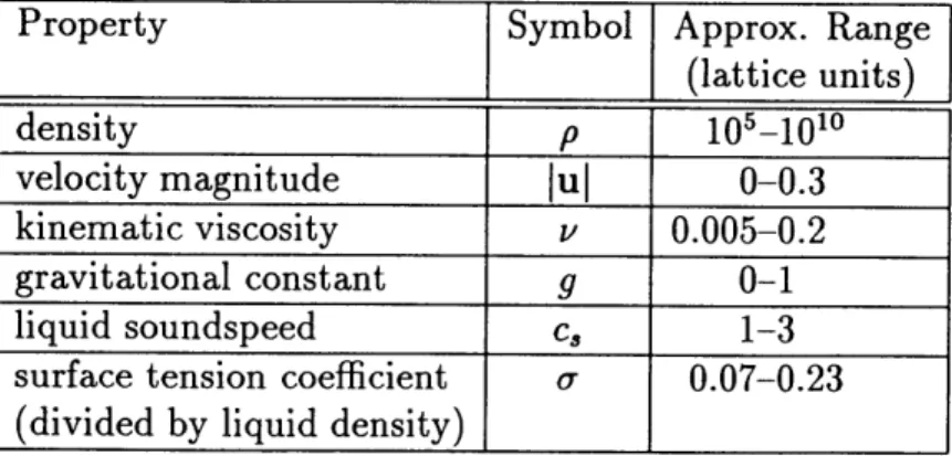
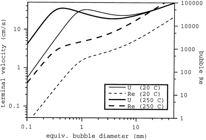
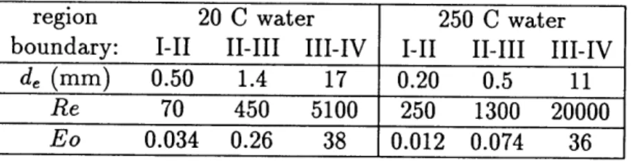
5.1 Bubble rise behavior, water at 20 C and 250 C . . . .

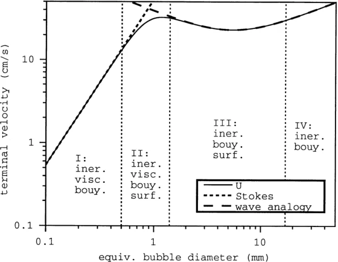
5.2 Regions of bubble rise behavior . . . .

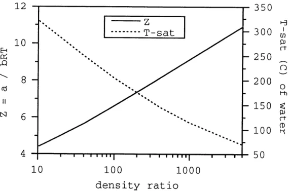
5.3 van der Waals parameter Z and T,,t of water vs. density ratio

5.4 Reduced temperature vs. density ratio . . . .

5.5 Reduced pressure vs. density ratio . . . .

5.6 Dimensionless latent energy vs. density ratio

5.7 _{Dimensionless latent entropy vs. density ratio}

. . . . . 1 1 8 118 . . . . . 119 . . . . . 119 . . . . . 29 . . . . . 31 . . . . . 43 48 102 103 117

(9)

5.8 Dimensionless latent volume-work vs. density ratio

5.9 Dimensionless liquid and vapor soundspeeds vs. density ratio .

6.1 Species populations vs. internal energy per unit mass u . . . .

6.2 Stability test results . . . .

6.3 Flowchart of algorithm ...

7.1 Example of shearwave test results . . . .

7.2 Examples of soundwave test results . . . .

7.3 Density profile of liquid compressed by gravity . . . . .

7.4 Spontaneous phase separation . . . .

7.5 Average densities during spontaneous phase separation

7.6 Planar two phase system setup . . . .

7.7 Density oscillations in initially phase separated system

. . . . . 187

191

192

194

196

7.8 Examples of oscillation frequency results . . . .

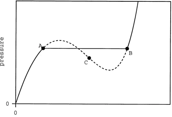
7.9 PV diagram - coexistence curve . . . .

7.10 Results of surface tension measurement via Laplace's Law . . .

7.11 Surface tension measurement: (PN - PT) across a flat interface .

7.12 Density profile across a flat interface . . . .

. . . . . 197 199 202 205 205 120 131 135 151 171 184 . . . . . 120

(10)

8.1 Rayleigh-Taylor instability . . . .

8.2 Example of bubble rise simulation . . . .

8.3 Illustration of bubble size determination . . . .

8.4 Example of height vs. time results and terminal velocity calculation .

8.5 Rise curve and bubble shape contours for spherical bubble

8.6 Rise curve and bubble shape contours for ellipsoidal bubble.

8.7 _{Rise curve and bubble shape contours for cap bubble...}

8.8 _{Rise curve and bubble shape contours for another cap bubble .}

8.9 Terminal velocity vs. bubble size results - lattice units . . . .

8.10 Terminal velocity vs. bubble size results - real units . . . .

8.11 Dimensionless map of bubble rise simulation results . . . .

. . . . . 220 . . . . . 221 222 223 226 227 228 210 212 .. 214 217

(11)

List of Tables

5.1 _{Fluid and flow properties in the multiphase system}

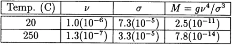
5.2 Properties of low and high temperature water . . . .

5.3 Bubble size regions in the behavior of rising bubbles .

6.1 Dynamic range of the (0, 1, 2, 1-v, -w) system . . . .

7.1 Shearwave test results . . . .

7.2 Analytical form of parameters in soundwave test . . .

7.3 Soundwave test results ...

7.4 Oscillation frequency results . . . .

8.1 2D bubble rise simulation results . . . .

97 ... . 101 . . . . . 105 130 169 182 183 ... 198 . . . 218

(12)

Chapter 1 Introduction

This thesis presents a lattice gas method for detailed simulation of two phase hydrodynamics. The method is an example of the "Digital Physics" approach to the simulation of physical systems governed by continuum mechanics. This multiphase Digital Physics system will be referred to as the "multiphase system" for short.

This chapter provides a brief introduction to two phase flow, lattice gases, and where the current method is thought to fit into each of these expansive fields. A summational outline of the thesis is provided as well.

(13)

1.1 Applications and Current Methods of Two Phase

Flow Modeling

Two phase flows of a gas-liquid mixture are extremely common, both in industrial processes and in nature. Chemical processes such as reaction or mass transfer are often carried out by contact of a liquid phase and a gas phase in a "chemical reactor." Over 60% of heat exchange equipment used in industrial processes involves two phase flow of one kind or another [1].

Large power production operations typically rely on boiling heat transfer, which results in a flowing two phase mixture of a liquid and its vapor. Study of the atmospheric and geohydrologic transport of materials often involves two phase flow. An important example is prediction of the fate of radioactive substances when evaluating disposal options. Another example is the petroleum industry, since methods of oil recovery typically involve multiphase flows.

One of the most active areas and important driving forces of two phase flow research for several decades has been the thermal-hydraulic design of nuclear reactors [2]. Safety and efficiency (in both the thermodynamic and economic sense) during normal operation require accurate prediction of two phase flow behavior. In addition, modeling of transient two phase flow is needed for safety analyses of possible accident conditions [3]. Especially in the latter case there is a diverse set of two phase flow problems that may come into play.

The most important feature of a two phase mixture is the presence of interfaces separating regions of one phase from regions of the other. Hence the flow has an internal structure, and the overall pattern characterizing the spatial distribution of the two phases is known

(14)

as the flow regime. For example, in vertical upflow through a conduit, the flow pattern is commonly regarded as belonging to one of the following flow regimes: bubbly flow, slug flow, churn (or froth) flow, or annular flow [4].

A basic problem in two phase flow modeling is that the important transfer mechanisms, between fluid and structure as well as between the two phases of the fluid, depend heavily on the flow regime. In turn it is often difficult to reliably predict the flow regime for a given system without direct experimental evidence. The fact that fluid properties, flow parameters, and system geometry are all influential in determining flow regime provides uncertainty in attempts to extrapolate from existing information [3].

In principle a two phase flow problem may be formulated in terms of the usual trans-port equations of single phase flow, with appropriate matching boundary conditions at the interfaces. With enough resolution this would allow direct computational prediction of the detailed flow dynamics, including the flow regime. Unfortunately this is far too computa-tionally burdensome to be practical, except for the very smallest of systems. Indeed the resolution needed for an explicit calculation of this nature is currently achieved only for a very limited range of single phase systems, which of course do not have the added complexity of spatially and temporally varying internal boundary conditions.

Practical two phase flow modeling (say for a nuclear reactor core) therefore requires a "macroscopic" approach where the interfaces are not explicitly modeled at all, but their influence on local transfers is accounted for by somehow adjusting the parameters and prop-erties of a simplified model. This is analogous to turbulence modeling in single phase flow, where the effects of turbulence are reflected in quantities such as the eddy viscosity. The

(15)

simplest and most common two phase flow model is the homogeneous equilibrium model (HEM), where the transport equations are solved for a single pseudo-fluid whose properties represent a mixture average of the two phases. The other approach is the separated flow model, in which each fluid is considered individually to some degree.

A very simple separated flow model is the drift flux model, which focuses mainly on the relative velocity difference (or slip velocity) between the two phases [5]. The drift flux model is especially useful because it requires modest computational work over that of the HEM, but can approximate flows where the fluids may have very different mean velocities. An example is annular flow, where an upflowing vapor core is surrounded by a liquid film whose net flow may be downward; here the homogeneous equilibrium model is clearly inadequate.

A more sophisticated separated flow model is the two fluid model, where the transport equations are written for each phase separately. Additional equations then describe interac-tions (such as rates of mass, momentum, and energy transfer) between the two phases and between each phase and the solid boundaries. Many forms of the two fluid concept exist, for example the energy transport equation may be written for the mixture while mass and momentum transport remain separate for each phase. The two fluid approach is common in current thermal hydraulics codes in the nuclear industry (e.g. [6]).

The choice of a model for a given system must strike a balance between computational speed and various degrees of accuracy and resolution. In all cases some level of fine grain detail is sacrificed, and the necessary approximations use information obtained empirically or semi-empirically. Most important in the choice and application of such information is knowledge of the flow regime. In correlating or theoretically formulating information used

(16)

in the parameters of the large-scale models, it is very useful to understand the physical mechanisms which govern the behavior in a certain flow regime and the transitions between flow regimes. It is in this capacity that modeling of smaller scale phenomena through theory, experiment, and fine grain computer simulation can play a valuable role. For example, correlations used in modeling bubbly or slug flow typically rely on prediction of the relative rise velocity of a single bubble.

Computational flow simulation in which the exact equations are solved as described above would offer a way, in compliment with experimental results, to intimately probe assumptions about basic physical mechanisms. To date the use of such simulations to investigate even relatively simple, small-scale two phase systems is quite limited because they are so com-putationally demanding. Progress in this direction has been made with the volume-of-fluid method [7, 8, 9] and the front tracking method [10] in the investigation of the motions of rising bubbles. Here the local instantaneous field equations (for incompressible fluids with no heat or mass transfer) are numerically solved, including an explicit dynamical representation of the interface as a discontinuity existing within specific volume elements. In one instance of recent work by Tomiyama, Sou, Zun, and Sakaguchi [11], 3D bubbly flow is simulated in a duct composed of - 2(104) cells. However, the flow is strictly laminar (Re < 100),

and values of certain relevant dimensionless quantities, particularly the Morton number, are far different than those representative of water. Nevertheless interesting phenomena have been studied with these methods, such as bubble deformation, lateral bubble migration, and patterns of bubble distribution resulting from the interaction of bubbles with the velocity profile of a shear flow.

(17)

The method presented here, the Digital Physics "multiphase system," recovers the exact equations for isothermal, compressible two phase flow. Its main usefulness, like any detailed simulation method, is expected to be found in the context of (a) providing insight into funda-mental physical mechanisms important in two phase flow behavior, and (b) better resolving the fine grain details of subsystems whose effects must ultimately be incorporated in an ap-proximate fashion into the coarse grain model for a large system. Moreover, the multiphase system is predicted to expand the range of two phase flow problems accessible to direct simulation of the detailed flow field including interfaces. This greater range refers to both the system size and the fluid properties, as represented through appropriate dimensionless quantities. The source of this optimism is an estimate of the computational performance of the multiphase system based on current commercial Digital Physics capabilities'. Simulation Reynolds numbers on order 104 _{are anticipated, which would allow study of, for example,} effects of turbulence on bubble dynamics. At the same time Morton numbers appropriate for water can be achieved. In addition, it may be possible to extend the multiphase system to allow simulation of non-isothermal flows (with very little additional computational work).

1.2 Lattice Gases and Fluid Flow Simulation

What is the multiphase system, indeed what is Digital Physics? The term Digital Physics refers to a fully discrete microdynamical system where mass, momentum, and energy are exactly conserved, entropy production is assured by a local H-Theorem, and the mean

(18)

havior recovers real continuum physics. A Digital Physics system capable of simulating low Mach number, ideal gas hydrodynamics is the multispeed lattice gas automata introduced by Molvig, Donis, Myczkowski, and Vichniac [12], and further developed by Teixeira [13], Chen [14], and others [15, 16, 17, 18, 19]. This ideal gas Digital Physics method will be referred to throughout this thesis as the "standard system." The multiphase system is an extension of the standard system which supports a non-ideal-gas thermodynamics appropri-ate for two phase coexistence; hence it is essentially a type of lattice gas automata.

In its most basic form, a lattice gas automata consists of identical particles which move about with unit speed from node to node on a fixed regular lattice. Associated with each par-ticle at any given time is a discrete velocity, also considered its microstate, which determines its direction of movement during the current step. Each complete update step consists of two events, a collision phase and a propagation (also called advection) phase. In the collision phase, particles have their velocities adjusted according to a set of collision rules; then the actual hopping to a new site comprises the propagation phase. At most one particle may exist at a given site with a given velocity, which is the "exclusion rule" of the lattice gas; hence a microstate is either occupied or unoccupied.

The collision rules are carefully constructed such that mass, momentum, and energy (and nothing else) are conserved for every collision. Of course when all particles have equivalent speed, then mass and energy are redundant. Collisions serve to randomize the local particle distributions, monotonically generating entropy such that the ensemble average occupation probability of any microstate has a value given by the local thermodynamic equilibrium2_.

(19)

The fate of the (average) occupation probability of a given microstate during a complete update step can be expressed as a difference equation, called the lattice update equation. The lattice update equation is Taylor expanded in space and time to give the microkinetic equation of the lattice gas. Then the mass, momentum, and energy moments of the microkinetic equation may be expressed as differential equations containing local macroscopic quantities, such as density and velocity, varying in space and time. These are the mass, momentum, and energy transport equations which describe the long-wavelength, low frequency dynamical behavior of the system.

This is analogous to the derivation of the real transport equations of continuum fluid mechanics from the Boltzmann equation. The first order Knudsen number expansion of the kinetic equation gives the Euler equations, and the second order expansion gives the Navier-Stokes equations. However, due to the presence of only a finite set of discrete velocities on the lattice, the transport equations of the lattice system will be different than those of true continuum mechanics. These differences are referred to as discreteness artifacts. In particular, the momentum flux tensor is generally anisotropic in a fashion related to the structure of the lattice.

In 1986 it was recognized by Frisch, Hasslacher, and Pomeau [20] that a 2D hexagonal lattice results in an isotropic momentum flux tensor for the lattice gas. This gives a momen-tum transport equation for the basic lattice gas just described which is similar to that of real hydrodynamics, but which still retains certain other discreteness artifacts. Nonetheless the discovery of the isotropic momentum flux tensor touched off a flurry of research into extensions of the original system [21, 22, 23, 24, 25, 26], the general theory of lattice gas

(20)

sys-tems [27, 28, 29, 30], and the potential to use them for hydrodynamic simulation [31, 32, 33].

Immediately investigated, for example, was the opportunity to exploit inherent computa-tional advantages of the lattice gas system [34], since each microstate could be represented by a single bit as the system evolved via simple logical and highly parallel operations. Shortly after the 2D hexagonal system was introduced, Frisch, Hasslacher, Lallemand, Pomeau, d'Humieres, and Rivet [35] showed that the face-centered hypercube (FCHC) lattice also results in an isotropic momentum flux tensor, and moreover could be used to represent a 3D system. A concept inspired by lattice gas automata called the "lattice-Boltzmann method" was developed [36, 37, 38], where the discrete particles are replaced with floating-point numbers, resulting in a kind of hybrid between a lattice gas and an explicit finite-difference scheme. In the decade or so since the landmark paper of Frisch, Hasslacher, and Pomeau [20], many other interesting and important developments have been made3

Most of the resulting lattice gas models, it turns out, suffer from the additional dis-creteness artifacts, limiting their usefulness as flow simulation methods. In 1988, however, Molvig, Donis, Myczkowski, and Vichniac [12] showed that a lattice gas composed of parti-cles with three different speeds, instead of just a single speed, could be designed to eliminate all discreteness artifacts from the momentum transport equation. By manipulating the dis-tribution of particles amongst the different available speeds (or energies) in a particular way, correct momentum transport is recovered exactly. In addition, this multispeed model, where mass and energy are no longer redundant, has a well-defined energy transport equation, with an ideal gas relationship between internal energy and pressure. This is the standard system

3

(21)

referred to above; certain discreteness artifacts remain in the energy transport equation, hence it is appropriate for simulating flows where heat transfer is not important.

The first demonstrations of the ability of the three-speed standard system to simulate quantitatively accurate 3D hydrodynamic behavior were presented in 1991 by Mujica [41] for flow past a flat plate, and in 1992 by Teixeira [13] for Poiseuille flow and flow past a circular cylinder. Teixeira [13] also showed that additional, higher particle speeds can be used to remove the energy transport artifacts, and that the FCHC lattice has the necessary symmetry properties to allow the inclusion of these higher speed particles4_{. Certain other extensions} to the multispeed lattice gas have been made, including the use of multi-bit microstate populations [16] (hence no exclusion rule). Larger populations drastically reduce the noisiness of the method, allowing a much crisper realization of the local instantaneous field equations of hydrodynamics. In order to equilibrate the multi-bit population distributions, the collision process [42, 18] at each site is carried out as a series of bilinear scattering events, in which each event drives the distributions closer to equilibrium5 _{. Moreover, this collision process} can be modified in a way that alters the shear viscosity of the lattice gas from its nominal value, hence the viscosity may be "dialed in" within a certain allowable range [17]. These and certain other developments6 _{have enabled the Digital Physics standard system to become a} powerful tool for simulation of low Mach number flows7 _{where it is acceptable to represent} the fluid as an ideal gas.

4In fact he proves that the momentum flux tensor remains isotropic for any particle speed of integer value

on the FCHC lattice.

5_{Which now has the usual Maxwell-Boltzmann form.}

6In particular developments related to high Reynolds number flow are not discussed here as they are

proprietary to EXA Corporation.

7

(22)

The presence of interfaces is the difference between a simple fluid and a complex one, such as a multiphase or multicomponent fluid. Several ideas for lattice gas models of com-plex flows have been put forth. A two component model called the "immiscible lattice gas" (ILG) was introduced by Rothman and Keller [45] in 1988, and recently another two component model using a lattice Boltzmann method was conceived by Swift, Osborn, and Yeomans [46]. A lattice gas exhibiting a liquid-vapor transition was formulated by Appert and Zaleski [47]. Various implementations and extensions of these, particularly of the ILG, have been explored[26, 48]. Generally, however, these methods not only retain the discrete-ness artifacts of single speed models, they also tend to have a very limited range of fluid-fluid density ratio and other key two phase properties. Recent work based on the ILG explores the use of "stopped particles" (particles of zero velocity) as a degree of freedom by which to remove one of the artifacts [49], or to increase the density of one component relative to the other [50]. The result, however, is that large amounts of stopped particles severely limit the fluid velocity. Furthermore, the equation of state in such systems (i.e. the pressure-density relation) is quite unphysical, in fact the liquid is actually more compressible than the gas.

A particularly interesting concept was introduced by Shan and Chen [51] in 1993 in their multiphase lattice Boltzmann model. They formulated a non-local, nearest-neighbor interaction that mimics an interparticle "potential," and in the macroscopic limit yields a non-ideal-gas equation of state. The interaction alters the local value of momentum at a site in a way that reflects its neighborhood, but does so in a fashion that conserves momentum globally (i.e. over the lattice as a whole). The equation of state can be tuned by adjusting a parameter central to the non-local interaction, and two phase coexistence occurs when the

(23)

pressure-density relation exhibits a hysteresis such that two different densities are stable at the same pressure. This concept was used with a single speed lattice Boltzmann method, where discreteness artifacts in the momentum equation can be eliminated, but there is still no energy degree of freedom; hence any connection with two phase thermodynamics is hindered. Also, lattice Boltzmann methods are subject to numerical instabilities [52] because they use floating point values rather than discrete particles.

In the present work a discrete adaptation of the non-local interaction concept of Shan and Chen is developed as an extension to the Digital Physics standard system. This requires construction of an exact-integer version of the sitewise momentum adjustment process, the addition of a new microphysical feature to account for the energy associated with phase change, and several other developments which are detailed herein. The result is the first lattice gas method with correct momentum transport, two phase capability, a realistic equa-tion of state for the gas and liquid phases, and the ability to achieve liquid-vapor density ratios sufficient for simulation of practical systems. Furthermore, the independent energy transport equation provides the potential to extend the method to include heat transfer. This work also contains the first application of a lattice gas method to the investigation of two phase bubble dynamics.

1.3 Outline of Analysis

The goals of this thesis are as follows. The first is to present the fundamental extensions which allow the multiphase system to obey a more general equation of state than that of an ideal gas,

(24)

specifically one which exhibits a region of two phase coexistence. The second is to show how to recover correct hydrodynamical behavior for the resulting individual bulk fluid phases. The third is to outline the potential for the multiphase system to provide quantitatively accurate simulation of real fluids, particularly water, in two phase flow situations of practical interest. The fourth is to present experimental results for a 2D version of the multiphase system which verify the theoretical predictions for the properties of the multiphase system, and demonstrate its ability to capture certain key physical mechanisms of two phase flow.

The content of this thesis is intended to introduce the fundamental advances leading to development of the multiphase system, and to investigate its properties primarily from the perspective of achieving correct two phase hydrodynamics. The multiphase system is in principle capable of modeling a variety of substances over a range of (equilibrium) thermody-namic conditions. The specific implementation presented here is intended to be as simple as possible but nonetheless suitable for an approximate representation of water. It is also a 2D version, but the extension of the multiphase system to 3D is entirely straightforward; 2D was used only to speed development of the fundamental algorithms by reducing computational requirements as much as possible.

A key limitation of the multiphase system at present is a maximum liquid to vapor density ratio of about 200. Another important limitation in the present implementation is the required use of an "isothermal condition", where all of the material in the system is imagined to be in immediate and instantaneous contact with a constant temperature reservoir. These restrictions are likely associated with the need for additional microphysics within the finite interfacial region. While heat transfer issues are beyond the scope of this project, the ability

(25)

to include heat transfer in the multiphase system is feasible if a way to eliminate the need for the isothermal condition can be found. The multiphase system does take important steps towards heat transfer capability. It includes a physically consistent representation of thermodynamical quantities, emphasized for example by the large difference in internal energy per unit mass between the vapor and liquid phases. Furthermore, it is believed that the energy transport analysiss _{provided in this thesis is sufficient to construct a method for} single phase flow of a non-ideal-gas vapor or liquid including heat transfer, although this task has not been undertaken here.

The remainder of this document is organized as follows. In Chapter 2 a new operator, named the interaction operator, is introduced into the Digital Physics microsystem. The interaction operator is shown to provide a non-local interaction, in the form of a sitewise momentum and energy adjustment, which mimics the intermolecular forces in a real liquid. Chapter 3 discusses how the momentum piece of the interaction operator gives rise to non-ideal-gas behavior, and in particular can be used to achieve a thermodynamical system, such as a van der Waals system, appropriate for modeling two-phase coexistence. It also introduces the "microscopic internal energy" as a means to address the internal energy dependence in the multiphase system, which must account for the latent heat of the liquid-vapor phase transition. In Chapter 4, the moments of the resulting microkinetic equation are evaluated at the Euler level to provide constraints by which to remove discreteness artifacts. Correct momentum transport requires the same constraints as in the standard system. On the other hand the energy transport equation contains new artifacts, one of which must be removed

(26)

using the energy piece of the interaction operator. Although it is shown how to recover correct adiabatic energy transport for the multiphase system, in practice the isothermal condition is needed in the two phase simulation experiments.

Chapter 5 looks at the important thermodynamic and flow properties involved in modeling two-phase flow of water, and describes the relationship between macroscopic quantities in the lattice system and those of the real world. It also discusses predictions of the capabilities and limitations of a 3D, "engineering-scale" multiphase system for simulating flow systems of practical interest, and bubbly flow is identified as a promising application. Chapter 6 addresses key issues in selecting and implementing a specific multiphase system. These include solution of the system of constraints needed to remove artifacts, and a modified advection scheme required to stabilize the liquid phase due to its elevated soundspeed. Also included is a description of the algorithm used in the 2D simulations presented in this thesis. These experiments and the results are described in Chapters 7 and 8. In Chapter 7, the more basic behavior of the multiphase system is observed and compared to theoretical prediction. This includes single phase shearwave decay and soundwave propagation tests, spontaneous phase separation, and experiments which probe the equilibrium properties of two-phase systems at rest. Chapter 8 looks at simulations of two dynamic liquid-vapor systems: Rayleigh-Taylor instability, and single bubble rise in a column of liquid. Chapter 9 presents conclusions and further discussion of a few key issues.

(27)

Chapter 2 The Multiphase Microsystem

2.1 A Non-Local Interaction

This chapter begins the theoretical description of the multiphase system by introducing and describing its microdynamical nature. In particular, the goal is to show how the set of microscopic rules which constitute the standard system can be extended so as to achieve multiphase behavior in the macroscopic limit. The thermodynamics of the standard system are consistent with those of an ideal gas. The fundamental advance by which multiphase behavior will be brought about for the new system may be viewed as the existence of non-ideal-gas thermodynamics, which is a physically consistent basis. However, rather than imitating the highly complex molecular interactions which result in the real non-ideal-gas behavior of a substance, a simple, discrete microscopic procedure in the usual Digital Physics

(28)

fashion is desired. This chapter will be concerned with motivating and formulating such a microscopic procedure.

In a real fluid, the departure from ideal gas behavior is a result of the forces exerted on the fluid molecules by other fluid molecules. Due to these forces, at any instant in time the motion of a particular molecule is influenced by the relative types and positions of the molecules around it. In a gas, the molecules are far apart, and intermolecular forces are weak relative to the mean molecular kinetic energy. On the other hand the molecules of a liquid are held close together by attractive intermolecular forces and very short range repulsive ones, and these interparticle forces dominate the instantaneous molecular motions.

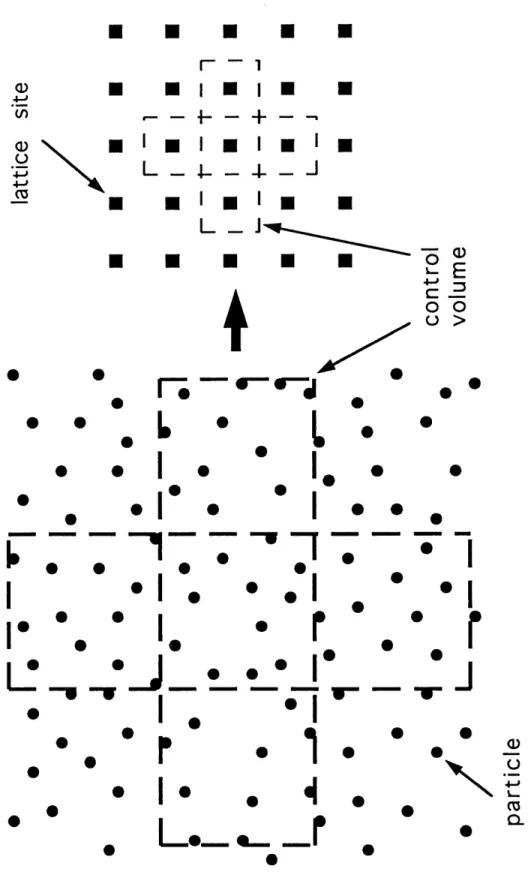
This physical picture points to the idea that to achieve a Digital Physics representation of a fluid with non-ideal-gas behavior, such as a liquid, an interaction should be introduced through which a lattice gas particle "feels" the other particles around it. Particularly within a liquid phase the interparticle interaction should be very strong. There is a fundamental difficulty with such a concept, which is illustrated in Figure 2.1. Consider the collection of particles drawn on the left-hand side. If these were the molecules of a real material, then the influence of one particle on another would depend on the distance between them. In a lattice gas, however, the system is spatially discrete; one can imagine drawing control volumes (shown by dashed lines) which fill space, and every particle belongs to exactly one of these unit cell microvolumes. Most significantly, all the particles of a cell are represented as existing at a central node, hence all information is lost concerning the precise locations of particles within a cell. Naturally the set of control volumes forms the lattice, and their central nodes are just the lattice sites, as shown on the right side of Figure 2.1.

(29)

m m m m m

L-r - -- 1

gl

Ig

l

g

L

J

Co 0 0 U >

T

*

l

* L

*

.

0 I

0

I. r

e· I I

• -7- 7 " 1 '2 -

II

0 a

I

SI • • • I

,, ,

_*

_I

_r

.

0 1 I - I

-.

4

a, I' ('3 0a L@muum.. m..inmmm..t

Figure 2.1: The lattice gas - a spacially discrete collection of particles. a) 4-J

a,

4-, ,A.ýý J • •m A

(30)

In the lattice gas, precise particle locations by which interparticle distances could be determined are not available, instead there is only the discrete distances between lattice sites. This suggests replacing interactions between particles with interactions between sites, where now one site "feels" the other sites around it through their local macroscopic properties such as density. A conceptual illustration is provided in Figure 2.2; the first part shows forces between molecules of a liquid, the second shows momentum exchange between sites with different densities (indicated by the patterns). In particular, one can imagine momentum exchanges between pairs of sites which increase with the product of the densities of the pair. However when that product becomes very large (such as between the two highest density sites in Figure 2.2), the amount of momentum exchange begins to decrease, essentially representing repulsive forces at very high density. The physical interpretation is that a mean interparticle distance in a local neighborhood of lattice sites is found by examining the densities of those sites. Then variations over its neighborhood give rise to the forces experienced by a given site. In this way one can hope to capture the physics of a liquid through a mean-field approach in a spatially discrete system.

A distinguishing feature of such a lattice gas is the presence of a non-local interaction, since in carrying out the microdynamics at one site, information about other sites is employed. The implementation of such an interaction must be some new operation or set of operations which alters the microscopic population distribution of a site in response to the influence of its neighbors. Moreover, it is believed that in general such operations must locally alter one or more of the fundamentally conserved quantities -mass, momentum, and energy. A simple argument may be made for why this should be true. Consider the nature of the standard

(31)

Sas

..

...

4 .*..

I

--

,

r

:-ass age

I'A

'r

:.'.:.-

..

,

aT ar' "a" 8 --

L

i...

assuage

T.

· ".

rr

"

.

r2:'

-. I,

0

0 Q

)

0 ar

6

0

bD+ cd

O-Xý

--O

(32)

system, which consists of two operations, a propagation step and a collision step. The purpose of collisions is to force the distribution of particles at each site to be the Boltzmann distribution. This maximizes the local entropy for a given mass, momentum, and energy, which must be the only invariants of the collision process. At the completion of a successful collision process, the distributions are at (or very near) equilibrium, and the propagation step must act on these equilibrium distributions in order to recover hydrodynamics at the macroscopic level. Thus any other operation must act after the propagation step but prior to the collision step. However, if an operation acting at this time were to alter the distributions in some way but did not affect the invariants, there would be no net effect at all, since the following collision step would destroy any trace of the operation when it restores the equilibrium distributions.

Thus the purpose of the non-local interaction, indeed the only way it can be meaningful, is to break sitewise conservation of some combination of mass, momentum, and energy. In keeping with the principles of Digital Physics, however, exact integer conservation is required in a global sense, that is to say the total mass, momentum, and energy of the whole system must be constant in the absence of external influences. In order to ensure this, it is desirable to design the new operations to represent some sequence of events, each of which conserves mass, momentum, and energy individually. This implies that each hypothetical event is some sort of exact exchange process of one or more of these quantities. This concept is employed in Section 2.3 (and 4.2) when the precise nature of how to implement the non-local operations of the multiphase system is explored.

(33)

2.2 The Interaction Operator

In this section a general formalism for a Digital Physics system which can include the ex-change of mass, momentum, and energy amongst neighboring sites will be developed. This formalism must provide a microscopic description of the system from which its macroscopic behavior can be derived. It is useful to first recall briefly some basic properties of the stan-dard system, which forms the framework for the multiphase system. The underlying lattice is the 4D face-centered-hypercube (FCHC) lattice, which possesses certain necessary sym-metry properties [27]. Particles move from one lattice site to another according to their discrete microscopic velocities during the propagation phase. Then particles at the same site exchange momentum and energy during the collision phase, where each collision event conserves mass, momentum, and energy exactly. For each site, the collisions cause the distribution of particles amongst the available velocities to be that representing local ther-modynamic equilibrium1_{. The system evolves by repeated updates of propagation followed} by collision. It is not very difficult to imagine that the system just described represents a discrete version of an ideal gas.

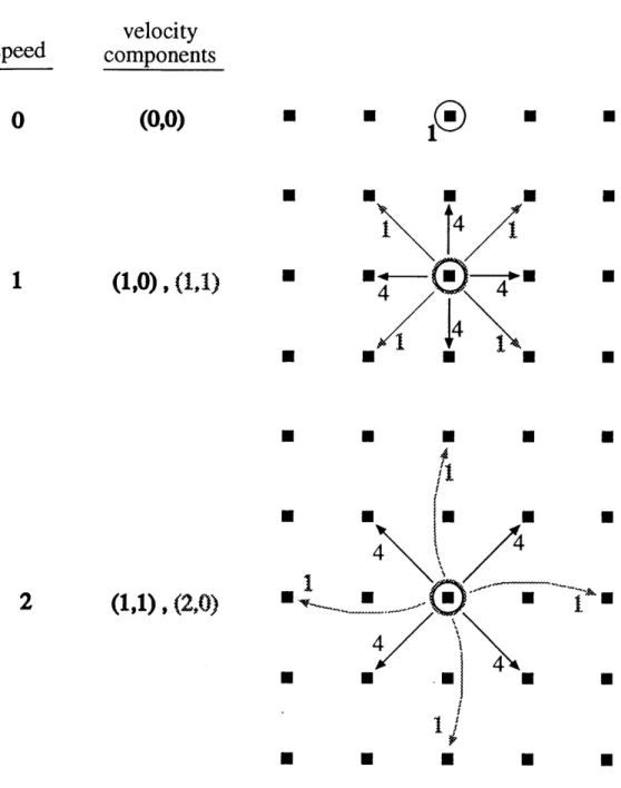
At least three different speeds of particles are required in order to recover correct momen-tum transport. The nominal (three-speed) version of the standard system contains particles of speed 0, 1, and 2. The speed of a particle is actually its microscopic kinetic energy

ej = mcy/2, where m is microscopic mass and cj is the microscopic velocity magnitude. The

microscopic velocity vector cji gives the direction and distance that a particle travels during 'A theoretical description of the original lattice gas collision operator is given by Frisch, Hasslacher, Lallemand, Pomeau, d'HumiBres, and Rivet [35]; _{the collision process developed for the multi-bit states of} Digital Physics is discussed by Chen, Teixeira, and Molvig [19].

(34)

the propagation phase. The notation of Molvig, Donis, Myczkowski, and Vichniac [12] is continued here, using j to refer to the particle speed (or more generally species) and i to refer to a specific velocity available for that speed. The vectors representing the possible velocities for speed 0, 1, and 2 particles are shown in Figure 2.3 for a 2D mapping of the FCHC lattice. This set of vectors is the one actually used in the 2D implementation of the multiphase system for this thesis. The numbers by the arrows indicate the degeneracy or "weight" associated with a velocity; weights occur due to the representation of a 4D system in 2D.

The basic mathematical description of a lattice gas microsystem is its lattice update equation. The lattice update equation of the Digital Physics standard system2 _is

Nji (x + cs,, t + 1) - Nj; (x, t) = Cjj (2.1)

where Nji is the population of microstate ji at site x and time t, alternatively referred to as the microscopic distribution of state ji. As noted above cji is the velocity vector associated with microstate ji. Cji represents the collision operator C acting on the population at microstate ji, which causes that population to take its equilibrium value NjE_Q.

A new operator, the interaction operator I, is introduced as the formal representation of some non-local interaction within the Digital Physics microsystem. The interaction operator

2

(35)

velocity

components

(0,0)

(1,0), (1,1)

4

4 U

U

4 ·i

[

_{- ·}

_4m

4 U

M

Figure 2.3: Velocity vectors for speed 0, 1, and 2 particles on the 2D mapping of the 4D face-centered hypercube (FCHC) lattice used in Digital Physics. Numbers by arrows are degeneracy or "weight" of a microstate in the 2D representation of the FCHC lattice.

speed

0 _O

1

(36)

is included in the above equation to generate a new lattice update equation:

Nji (x + cji, t + 1) - Nji (x, t) = Cjj + Zi; (2.2)

where Zji is the interaction operator acting on the microscopic distribution Nji. Unlike the collision operator, which is purely local since it depends only on the distributions at site x, the interaction operator must somehow take into account information about the distributions at other sites in the vicinity.

To proceed it is helpful to get an idea of how the presence of this additional operator will affect the macroscopic dynamics of the system. A first order expansion (in Knudsen number, i.e. a small mean free path expansion) of the new lattice update equation gives

8,Nji + cji - VNj; = Cj; + ji; (2.3)

where Nj; (x, t) is abbreviated as Nj;, and then taking the mass, momentum, and energy moments:

Z

m [oNji + cj, . VNj, = Cji + Zji] (2.4)

Z

mcj, [atNji + cj,. VNji = Cjj + Zji] (2.5)

ji

Z

Ej [atNj, + cj,- VNj, = Cj0 + Ij,] (2.6) ji which go over to

8tp + V. pu =

+

Zi;,

(2.7)

ji

(37)

0tpu +

V

-H

•

₌

_ZTjicji

_(2.8)

ji

~w

+

V -

Qk

=

Z•Zij

(2.9)

ii

after employing the following definitions and relations:

m = _{microscopic mass (hereafter taken to be unity)}

ej = 1 mcj = microscopic kinetic energy

p = mNji = macroscopic mass (per unit volume)

ji

pu = ZmcjiNji = macroscopic momentum (per unit volume) ji

IIk = mcjicjiNji = PkI + gpuu = momentum flux tensor

Ji (2.10)

Pk = isotropic pressure

W = • jN; = E + 2plul2 = total macroscopic energy (per unit volume)

E = internal energy (per unit volume)

Qk = _jcjiNji = energy flux

mCji =

>

mcjiCji = EjCji = 0

ii i ji

Equations (2.7 - 2.9) express the "lattice Euler equations" for the multiphase system. They naturally look like those of the standard system, except for the terms involving the interaction operator I. For the moment let us assume that the momentum flux tensor

IIk

has the indicated form3

which is identical to that of the standard system (as derived by Molvig, Donis, Myczkowski, and Vichniac [12]). The subscript "k" used with the momentum flux

3

Actually the form given is for the zeroth order momentum flux tensor with Nji = NE Q

(38)

tensor, scalar pressure, and energy flux is meant to indicate that the given expressions for these quantities really represent only the "kinetic" contributions. Kinetic contribution or kinetic part denotes that part which is due to the conventional (ideal gas) part of the system and does not include the effects of the non-local interaction, which are entirely represented by the moments of the interaction operator written on the right-hand sides of these equations.

This is an important distinction since the non-local interaction is expected to provide a significant contribution to these quantities, indeed that is its function. Therefore the subscript "n" is used to indicate the so-called non-local contributions. The total quantities are the sums of the kinetic and non-local parts and will simply be written with no subscript, thus momentum flux II = ]Ik + I , scalar pressure P = Pk

+

P,, and energy flux Q =

Qk + Qn. By definition these total quantities must satisfy the Euler equations written as

tp + V -pu = 0 (2.11)

atpu + V - H = 0 (2.12)

atW + V .Q = 0 (2.13)

Subtracting equations (2.11 - 2.13) from equations (2.7 - 2.9) gives

• i-j = 0 (2.14)

(39)

Elij= V. Qk - V-Q = -V

-Qn

(2.16)

ji

These equations show that the mass moment of the interaction operator should vanish, and relate the momentum and energy moments to specific macroscopic quantities. It is therefore expected that local changes in momentum and energy, but not mass, will be required to occur between the propagation and collision steps. The way in which the amounts of these local changes in momentum and energy are calculated depends on the nature of the quantities V

- H

, the divergence of the non-local part of the momentum flux tensor, and V - Q,, the divergence of the non-local part of the energy flux. This analysis is dealt with mainly in the next two chapters.

For now the formal description of the interaction operator is continued by looking at how to implement the desired changes in local momentum and energy once they have been deter-mined. In the Digital Physics system, with its discrete particles and discrete velocity states, it is natural to think of "pushing" a particle from one state to another. The momentum and energy of a site will be altered by sequences of pushes at that site, where each individual push provides a small, discrete change in momentum and/or energy. Given the large state space associated with multiple speeds on a FCHC lattice, there are generally going to be a very large number of ways to push particles around so as to cause a given total change in momentum and energy. It is therefore useful to define a set of pushes P(A,pu, AnW) as any set that provides a momentum change of Apu and an energy change of A,W (where the subscript "n" denotes an effect of the non-local interaction). It is found then that Iji,

(40)

the interaction operator acting on the particles in state ji, can be written as

ji = AP [~iu(p) - (P)] _(2.17)

where a push of type p flips a particle from direction ji' to direction ji", Ap is the number of pushes of type p, and 6(P) is a Kr6necker delta function which is equal to one if ji = ji"(p), and zero otherwise (and likewise for S• •(P)). Substituting into equation (2.14),

>

2L i = A [1 ji ) -- ji(l(p

ji ji J P _(2.18)

=

A~~

j, - bj,

=E(P)]

A(1

-

1) = 0

P ji p

and it is seen that the mass moment vanishes as expected, since for every type of push the particles corresponding to direction ji' are subtracted and an equal number corresponding to direction ji" are added. The total momentum change is found by substituting into the momentum moment of the interaction operator,

S'(p)

C= c,

5

= AE ApC [&(P)

z[(p)

-

-ji ji P P ji (2.19)

=

ACjiI(,)

-

cji'(P= E Ac, =

A

pu

p p

where c, = cj;i,,() - _{cji,(p) is the microscopic change in momentum due to push p. Likewise,} the energy moment of the interaction operator gives

5

eji = E E A, [ --

'

Ej = Ape, = A,W (2.20)

(41)

where e, is the microscopic change in energy due to a push of type p.

The interaction operator as written in equation (2.17) has the appropriate form since its momentum and energy moments can be described as pushing operations which alter the momentum and energy at a site by specific amounts, while leaving the density unchanged. At this point it is useful to consider these new momentum and energy pushing operations as two separate entities, partly because they yield distinct macroscopic signatures, and partly because it is convenient to implement them as separate algorithms. In the following chapters, attention is turned towards the macroscopic considerations which govern the dynamically determined local instantaneous sitewise momentum and energy adjustments. First, this chapter further explores the formulation of the momentum pushing operation, which is the natural starting point of the non-local interaction.

2.3 The Interaction Force

This section addresses the concept of how to perform a sitewise momentum adjustment which inherently provides exact integer conservation of this quantity globally. It is useful to return to the idea of a sequence of hypothetical exchange events, each of which conserves momentum exactly. To make this concept more concrete, imagine that the particles throughout the lattice emit imaginary subparticles called "interactons" at each time step, and that the interactons emitted at one site are absorbed by the particles at other sites during the same time step. These particular interactons are massless and carry quanta of momentum. It is required that an equal number of these momentum-carrying subparticles are exchanged

(42)

between any pair of sites, where this number may depend on the local properties of those two sites such as density p and internal energy per unit volume E.

This construction suggests a pairwise "potential" Vpair between any two sites xl and x2,

Vpair, (X, X2)= GO" (xi) I (X2) (2.21)

where 0 = O(x) will be referred to as the "interaction parameter," and G = G (Xl - x2) is

a coupling coefficient which in general is a function of separation distance. Equation (2.21) has essentially the same form given by Shan and Chen [51] in describing their interparticle potential (they refer to 0 as the "effective mass"). The pairwise potential Vpair indicates the number of interactons exchanged between two sites. This number depends on the local properties of the two sites in a fashion determined by the functional form of the interac-tion parameter b; the macroscopic considerations which determine this functional form are addressed in the next chapter.

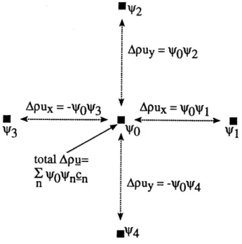
Naturally the pairwise potential should decrease with separation distance. This can be ac-complished by allowing the coupling constant G to decrease with increased distance between the sites. For simplicity and to minimize the range of the interaction (and corresponding computational effort), momentum exchange is allowed only between nearest neighbors, i.e. sites separated by a single velocity vector cji, and G is treated as a constant that is absorbed into the interaction parameter 0. It is further proposed that the momentum exchange be-tween a site x and its neighbor at x + cji is the pairwise potential Vp,,.i (i.e. the number of interactons exchanged) multiplied by the velocity vector cji which separates them. This

(43)

mV2

Apuy =

OV

2

Apux = -'O3 _Apux₌_l0O _i

V3

AO

V1i

total

Apu=

n _{Apuy = -'ON4}

mV4

Figure 2.4: Illustration of non-local momentum adjustment process

-

the net momentum

change of the center site is the neighborhood sum of the individual exact integer momentum exchanges.

implies that the total momentum change Aspu at site x may be calculated as the sum over

the neighborhood,

Anpu = >j Vpair (x, x

+

c;) cji =

Z

(x)b (x + c;i) ci; = _F(x)At _(2.22)

where the "interaction force" F has been introduced as equivalent to the local momentum change (which takes place over a time step At, thus F has units of force).

The interaction parameter b is a local macroscopic quantity determined dynamically for each site, then the momentum change at each site is calculated via the summation in equation (2.22). Figure 2.4 illustrates the momentum adjustment process, where it is pretended that

(44)

the nearest neighborhood for the site in the center consists of just the four other sites shown.4 This scheme, using the interaction parameter b to represent local properties, is the specific implementation of the concept pictured in Figure 2.2. The way in which the momentum at a particular site is influenced by its neighborhood has now been precisely specified. The form of the interaction force F given in equation (2.22) is the same as that introduced by Shan and Chen [51], _{except that the Digital Physics version involves exact integer quantities.}

It is straightforward to show that, as expected from its construction based on an exact exchange process, the interaction force conserves momentum globally. That is to say, the sum over all lattice sites of the momentum remains constant, because the sum over the lattice of the interaction force vanishes,

ZF(x) = 0 (2.23)

x

Following Shan and Chen, this is verified by writing

E F(x) = E 1 b(x)b (x + cji) cji (2.24)

x x ji

or, summing over -cji instead of cji,

- E F(x) = E E b(x)b (x - cj,) cji (2.25)

x x ji

but one may equivalently sum over x' = x - cji, which is indistinguishable from summing

4

The algorithm actually used in the multiphase system involves the 12 nearest neighbors representing speed 1 and 2 directions on the 2D mapping of the FCHC lattice, as described in Section 6.4.

A digital physics method for two phase flow