HAL Id: hal-00304592
https://hal.archives-ouvertes.fr/hal-00304592
Submitted on 1 Jan 2001
HAL is a multi-disciplinary open access archive for the deposit and dissemination of sci-entific research documents, whether they are pub-lished or not. The documents may come from teaching and research institutions in France or abroad, or from public or private research centers.
L’archive ouverte pluridisciplinaire HAL, est destinée au dépôt et à la diffusion de documents scientifiques de niveau recherche, publiés ou non, émanant des établissements d’enseignement et de recherche français ou étrangers, des laboratoires publics ou privés.
String of Beads model in time series mode
G. G. S. Pegram, A. N. Clothier
To cite this version:
G. G. S. Pegram, A. N. Clothier. Downscaling rainfields in space and time, using the String of Beads model in time series mode. Hydrology and Earth System Sciences Discussions, European Geosciences Union, 2001, 5 (2), pp.175-186. �hal-00304592�
Downscaling rainfields in space and time, using the String of
Beads model in time series mode
Geoffrey G.S. Pegram and Antony N. Clothier
Civil Engineering, University of Natal, Durban, 4041,South Africa Email for contributing author: [email protected]
Abstract
The String of Beads model is a space-time model of rainfields measured by weather radar. It is here driven by two auto-regressive time series models, one at the image scale, the other at the pixel scale, to model the temporal correlation structure of the wet-period process. The marginal distribution of the pixel scale intensities on a given radar-rainfall image is described by a log-normal distribution. The spatial dependence structure of each image is defined by a power spectrum approximated by a power law function with a negative exponent. It is demonstrated that this stochastic modelling approach is valid because the images sampled are effectively stationary above a scale of 30 km, which is less than a quarter of the image width. By advecting a simulated sequence of images along the same cumulative advection vector as the observed event and matching the image-scale statistics of each simulated image with those of the corresponding observed image, a simulated sequence of plausible images is generated which mimics (has the same space-time statistics as) the observed event but differs from it in detail. Aggregating the pixel scale intensities in each sequence over a number of time and space intervals and then comparing their spatial and temporal statistics, demonstrates that the model captures the intermediate scale behaviour well, showing satisfactorily its ability to downscale rainfall in space and time. The model thus has potential as an operational space-time model of rainfields.
Keywords: space-time, rainfield modelling, weather radar, multifractals, Gaussian random fields
Introduction
The String of Beads model was introduced by Pegram and Clothier (1999a, b and 2001). It is a stochastic model of a masked field of rainfall intensities measured by radar with a space resolution of 1 km over a circular area of 140 km radius and with a time resolution of 5 minutes — the time between radar scans. The particular weather system modelled here to check the downscaling properties of the model occurred during a wet January in 1996 and lasted 42 hours. This event was recorded by the S-band radar sited 20 km north-west of Bethlehem, South Africa.
Modelling rainfields in space and time has been the endeavour of hydrologists and physicists in the last four decades. Foufoula-Georgiou and Krajewski (1995) give a resumé of modelling approaches until 1994. A publication of particular interest is Bell’s (1987) approach where he showed (among other useful things) that rainfall values estimated by satellites obeyed a log-normal marginal distribution. Following Crane (1990), Pegram and Clothier (1999a, b) showed that radar-measured rainfield intensities
are described well by a log-normal distribution and confirmed, following a suggestion in Menabde et al. (1997), that the spatial correlation structure of a rainfield could be described satisfactorily by a power spectrum fitted by a power law. Menabde et al.(1997) showed that data-logging raingauges yielded short-duration rainfall sequences whose temporal correlation structure could also be described by a power law spectrum. These results suggested that the sequence of radar images of rainfield rates had a pixel to pixel correlation that could also be described by a power spectrum with a power-law relationship (Pegram and Clothier, 1999b). But those were preliminary results: the images the radar captured were of an advecting field and, therefore, the estimated temporal spectrum was not “true”. Marsan et al. (1996) drew attention to the need for modellers to give proper attention to the anisotropy of the scaling behaviour of rainfields in space and time, addressed the problem of advection and derived a causal model using Fourier transforms. More recently, Seed et al. (2001) have modelled the space-time behaviour of radar images, capturing part of an extreme rainfall event during a hurricane
off Darwin, Australia. The modelling approach they used was a seven-level multiplicative bounded (multi-fractal) cascade which simulates seven different spatial scales independently. Each level was linked pixelwise to the same level at the next time step via a different ARMA(1,1) model. Rainfields are then simulated by summing contributions from each of the seven scales.
The former version of the String of Beads model (Pegram and Clothier, 1999a, b and 2001) exploited the concept of power-law filtering of Gaussian random fields in the space domain and also in the time domain, by exploiting Taylor’s (1938) hypothesis, to capture the correlation structure of the rainfall process. In power-law filtering a Gaussian noise field, the technique is to transform the noise field into Fourier space and then to multiply each term in the transformed field by a filter function which is defined in Fourier space by a power-law relationship. The product field is then inverse-transformed into real space; this operation has the effect of performing a convolution of the filter function and the noise field. This is the technique used in the generation of universal multifractals (Schertzer and Lovejoy, 1987) and the result is a spatially correlated noise field. The ideas of Marsan et al. (1996) and Seed et al. (1999) suggested that a one-layered image could be linked in time by a pair of high order Auto-Regressive models (rather than a cascade of ARMA(1,1) models or a modified power-law filter) to give the correct temporal correlation structure.
The two time series models in the new version of the String of Beads model presented here are applied at two levels: to the image mean flux (IMF) and to the pixel scale intensity (PSI). It is proposed that the spatial power law filtering then ensures that the generated images, used in either simulation or now-casting applications, scale correctly in space and time.
The main objective of this paper is thus to present the most relevant aspects of the “String of Beads” model in the context of downscaling of rainfall and to illustrate the model’s ability to capture this behaviour. The theme of the paper is developed in three parts: the first describes the time series form of the “String of Beads” model, a modification of the authors’ previous work and to describe the data analysis and the generation methodology. The second part is to report on a simulation of a 42-hour rainfall event based on the statistics of the observed images and then to compare the statistics of the various space-time aggregated rainfall intensities/amounts of the sequences of simulated images to that of the observed. In the final part, conclusions are drawn as to the performance of the “String of Beads” model in terms of the downscaling behaviour of its output.
Description and analysis of the
bead component of the model
The String of Beads model (SBM) gets its name from the concept that the wet-dry process on an area of interest is a one-dimensional time series (the “string”) which can be modelled by a Markov chain (if time is measured in discrete intervals) or by an allied alternating renewal process in continuous time (Cox and Miller, 1972). The Markov chain has been dealt with elsewhere (Pegram and Seed, 1998) and interest herein is confined to the wet period process, which has dimensions of 2-space + time, and constitutes the “Bead” on the “String”.
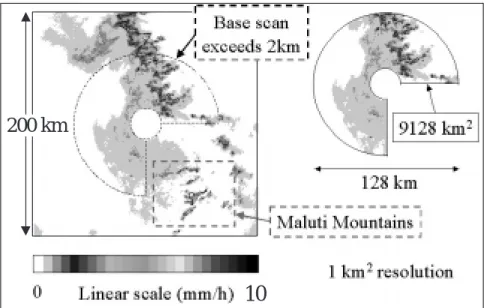
Each radar image of rain-rates measured every five minutes in the data-set supplied by the South African Weather Bureau (SAWB) has a typical radius of 140 kilometres, cropped to a 200 kilometre square. In this study, the area of analysis was limited to a radius of 64 km within which the data were judged to be reasonably sound for many technical reasons (level of base-scan, partial beam filling, bright band, etc.); also the dimension being a power of 2 facilitates the use of the Fast Fourier Transform. An example of a masked radar image is presented in Fig. 1a. The mask is a ¾ dough-nut shape because data were not captured until some distance from the radar and there is a region of large permanent reflectivity from the Maluti Mountains in Lesotho, south-east of the radar.
The number of pixels in the masked area is 9128, each 1 km square. The rain rate data were stored in integer form, so that a pixel with a zero entry might have been either dry or have experienced light drizzle. The imprecision of this 8-bit integer format does have a negative influence on the analysis procedures which will be noted where appropriate. The data were supplied in this form due to storage constraints although this has since been changed and full precision data are now available.
The model of the Bead adopted in this paper can be summarised as follows. Each masked image is treated as a sample from an exponentiated, spatially correlated Gaussian field. Each image’s pixel scale intensities (PSIs) are therefore modelled by a log-normal distribution, described by two parameters, which vary from image to image. The spatial correlation structure is modelled by a simple, homogeneous, isotropic power-law spectrum described by one parameter. The temporal structure between images is modelled at two levels; the image scale and the pixel scale. At the image scale, the image mean flux (IMF) and the wetted area ratio (WAR) are related functionally to the parameters of the lognormal distribution describing the PSI.
Now, in operational or simulation mode, the IMF and WAR are modelled by a bivariate AR(p) process and the
slope of the power spectrum is treated as constant. However, these aspects of modelling the space-time process are avoided in this paper because the historical image scale statistics are used as the basis to recreate an alternative PSI history to make valid comparisons between the scaling characteristics of the model and the observations. At the pixel scale, the temporal correlation structure is also modelled as an AR(p) process, but at this level it is the same univariate model applied to each pixel sequence in turn. The statistical interrelationship between the pixels is supplied by the power spectrum.
The difficulty of this approach is that the radar measurements are of rainfields, which are usually advecting past the radar at various speeds and directions by the weather. To extract the PSI time series structure requires working in the Lagrangian or the Eulerian reference frame. The first requires the alignment or shifting of the images by maximising the temporal correlation. The second requires coping with an advecting field. Both were tried: the first approach failed (although it will be reported and reasons given for its failure) and the second requires calibration. Any space-time model of rainfields must tackle the problem of advection to capture the PSI correlation structure. What has been developed and is proposed (in the time-series approach) seems to be a sensible and effective method (if at this stage cumbersome), as will be demonstrated. It is hoped that the method will be streamlined and simplified in future. The image scale analysis proceeds as follows. A rain rate estimate averaged over a given pixel site u, where u has
position (xu, yu) in the two-dimensional field, is a realisation
x(u) of a random variable X(u) sampled from an underlying
10
200 km
Ra d ia lly a ve ra g e d tw o d im e n sio n a l sp a ti a l p o w e r sp e ctru m P (f) = c. f -2. 43 1 10 100 W a v e n u m b e r f S p ec tr al d en si ty P (f ) 103 109 108 107 106 1 05 104Fig. 1a. Masked radar image of rainfall
Fig. 1b. Radially averaged two-dimensional power spectrum of
radar-rainfall image
random field. The ranked and binned (integer) data x(u) are assumed to be drawn from a log-normal distribution with
parameters σ and µ. After obtaining estimates s and m of
these parameters, applicable to a given image, the individual pixel values are normalised and standardised as y(u) = [ln{x(u)} – m]/s where if a value of x(u) is zero, y(u) is set to –3. This is one of the serious limitations of working with integer data — there are others which will be mentioned where appropriate. The image of y(u) values is then Fourier transformed to Y(f) and its power spectrum p(f) calculated;
this is described by p(f) ~ f -β . The negative β exponent,
here called βspace , is obtained by averaging the power
spectrum radially, assuming isotropy, and takes values typically in the range 1.9 to 2.6. The spectrum and its power law approximation are shown in Fig.1b; the marginal
distribution is shown as a survivor function in Fig. 1c where a very good fit is obtained until 2% exceedence probability, the model tending to slightly over-estimate the probabilities in the tail.
Returning to the analysis, the field Y(f) is inverse
power-law filtered using the value of βspace estimated from it (note
that inverse law filtering of a field is similar to power-law filtering, only the field is divided by the filter function and the result is a field with reduced spatial correlation); it is then inverse Fourier transformed to a field whose individual pixel values are labelled z(u), constituting a random field of pre-whitened rain rates still with temporal structure. If the assumption of lognormality of the PSI field x(u) is correct, z(u) should be Gaussian. However, due to the integer nature of the data, the marginal distribution of the field z(u) has extremely high kurtosis, so before the temporal correlation structure can be studied, a normalising transform following the ideas of Zucchini and MacDonald (1999) needs to be applied to the 9128 z(u) in each masked image. This involves ranking the z(u) values, associating cumulative probabilities with each element as if they were drawn from a uniform distribution and then transforming them to normality in the usual way.
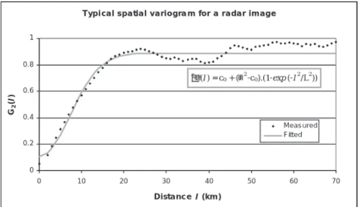
To examine the spatial dependence structure in more detail, the variogram of a typical image is shown in Fig. 1d. The variogram is computed by taking the ensemble average of squares of differences of z(u) values separated by l, which is the same as the second order structure function
G2(l) = where l is the displacement
from u. A model of the variogram is fitted to the data as shown in Fig. 1d where two points are worth noting. First,
there appears to be a distinct nugget effect c0 , or shift at the
origin, meaning that there is inherent error associated with measuring of z(u) values. This nugget effect affects the modelling process, so that, in simulation, extra noise must be added at the pixel scale or else the sequence of images is
too smooth. Second, it will be noted that the variogram flattens off after about 30 km from the origin, indicating
that the values of G2(l) tend to the variance σ2 of the field,
in turn implying that the field is stationary (Cressie, 1991) at a scale intermediate between pixel and image. The significance of this observation is that for the 128 km-square images which the SBM is designed to simulate, treating the images as stationary random fields and using traditional stochastic tools in the analysis, as done in the SBM, is a legitimate approach.
Correlations in time are affected by the advection of the storm across the window of the mask; therefore, it is important to find the image-to-image displacement history of the storm so that it can be mimicked faithfully. It is also necessary to remove the effects of advection by aligning or spatially translating the successive images until maximum serial correlation is achieved so as to determine the PSI correlation structure of un-advected images in the Lagrangian frame of reference.
Aligning the images is accomplished via a pattern search in a discrete domain, which is illustrated in Fig. 2. Consider two consecutive images. First, the pixel-to-pixel cross-correlation is computed for the images with no spatial shift. The images are then shifted diagonally relative to each other to each corner of a 9 km square simplex and the correlation between the PSIs of the images at each shift is computed. The correlations computed at each of the five shifts are then compared and the shift corresponding to the highest correlation is chosen as the centre for the new simplex. This is repeated until the highest correlation is at the centre of the simplex, at which stage the shifts corresponding to the two highest correlations in the simplex become the corners of a new simplex, half the size of the original (i.e. a 5 km simplex). The process continues until the size of the simplex is 1 km and then the correlations of the eight surrounding pixels are computed to find the maximum of the
cross-T yp i ca l sp a tia l v a ri o gra m for a r a da r im a g e
0 0.2 0.4 0.6 0.8 1 0 10 20 30 40 50 60 70 D ista nc e l (km ) G2 (l ) Meas ured Fitted 2γ(l ) = c0 + (σ 2 -c0).(1-exp (-l 2 /L2))
Fig. 1d. Estimated variogram of typical radar image and fitted
function 2 ) ( ) (u l z u z + −
C o m p a riso n o f su rviv o r fu n c tio n s o f th e m a rg in a l d istrib u tio n o f ra in fa ll ra te o n a ra d a r i m a g e 0.00 1 0.0 1 0.1 1 0 5 10 15 20 25 3 0 35 40 Ra i n fa ll R a te (m m /h ) P r o b ab il it y o f ex c ee d e n ce M easured Fitt ed
Fig..1c. Comparison of the survivor functions of the observed and
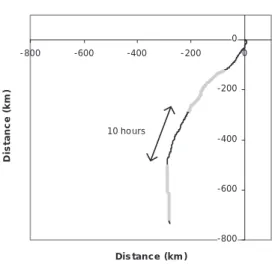
C u m u la tiv e a d v e c tio n v e c to r -800 -600 -400 -200 0 - 800 -600 -400 - 200 0 Dis ta n c e (k m ) D ista n ce ( k m ) 10 ho urs
correlation between the images. The algorithm is a form of two-dimensional bisection search, on a square simplex, which is extremely fast on a correlation field which is usually unimodal. The best guess for the next consecutive pair of images is taken as the correlation shift of the previous pair. Once the relative inter-image shift has been optimised (of course, accurate only to the 1 km scale of a pixel), the accumulative vector of displacement of the successive images from the first can be determined. For the event studied, this cumulative advection vector is displayed in Fig. 3. To give an idea of time scale, the alternating shaded segments on the track are each 10 hours long.
As mentioned above, an attempt was made to determine the PSI time series structure from the aligned images, but
Fig. 2. Schematic of 2-dimensional bisection search algorithm employed to find displacement of maximum correlation; starting with squares of
9x9 pixels and ending with 3x3 to confirm the maximum at pixel scale. Contours of a fictitious spatial cross-covariance function are superimposed.
Fig. 3. The cumulative advection vector, built up from image to image shifts, each optimising cross-correlation between successive
images using the search algorithm of Fig. 2
this proved unsuccessful, because the approach resulted in measured correlations which were too small to generate realistic sequences of images; in spite of its failure, the (seemingly straightforward) methodology attempted will be described briefly.
The cumulative advection vector of Fig. 3 was used to align the pre-whitened z(u) images so that when viewed as an animated sequence, the storm appeared to be still in space, but growing and decaying. In the artificially “still” Lagrangian storm reference frame, the mask appeared to move. In this next step of the analysis, sequences of PSIs sampled from consecutive images at a point in the Lagrangian reference frame, were analysed. Because of the occluding effect of the (now relatively moving) mask, there were many short sequences and few long ones. In the sequence of images analysed, which had moderate advection velocities of between 10 and 40 kph, it was possible to collect 13400 sequences of PSIs 64 images (320 minutes) long for analysis. These did not all start at the same time but, assuming ergodicity, were analysed individually and their serial correlation coefficients at each lag averaged to give an ensemble correlogram out to a maximum lag of 180 minutes. The Fourier transform of this PSI correlogram yielded a spectrum with a negative power-law exponent of
btime = 0.24, which is very small — it is a spectrum close to
that of white noise. This approach was abandoned as a means of determining the serial correlation structure of the PSI and a different approach was adopted as described presently, in which it is combined more appropriately with the simulation procedure upon which the determination depends. The modelling of the image scale statistics will be described first.
At the largest scale, the image mean flux (IMF) which is closely related to the wetted area ratio (WAR) is given as
exp(µ + σ 2/2) where µ and σ are the two log-normal
parameters describing the marginal distribution of the PSI values on the image. There is an obvious advantage in exploiting this linkage for modelling purposes, which leads to the heart of this time series version of the SBM that is a space-time model driven by the time series model of the
IMF. It is possible to condition σ, µ and βspace at each time
step on the current value of the IMF and to ensure simultaneously the ensemble development of the average rainfall intensity at the image scale. The spatial correlation of the images (defined by the power-law description of the spatial power spectrum) ensures that the temporal time series structure of pixels of all intermediate space scales between
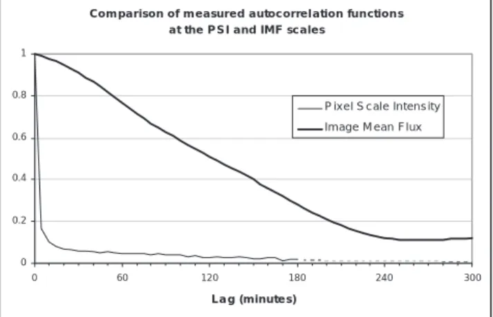
PSI and IMF scales is simulated realistically. The measured PSI temporal correlation structure determined by the abortive method described above and the IMF correlation structure are shown by the two correlograms in Fig. 4. As noted above, the measured aligned pixel scale correlogram does not have enough correlation to drive the time series structure of the model.
Each time series (PSI and IMF) can be modelled as an auto-regressive model of suitable lag p, of between 2 and 5 lags. The advantage of using an AR(p) model is that the innovation process is confined to one time step. It may not be the most parsimonious approach but, for modelling purposes, it is more convenient than a mixed ARMA(p,q) model for three reasons: ease of estimation, ease of generation and ease of forecasting; what is more, there is a plenitude of data from which to estimate the time series parameters. The Yule-Walker equations (Box and Jenkins, 1970) were used to extract the AR coefficients from the averaged sample correlogram. The order p was increased until a good fit to the correlogram as a whole was obtained in each case.
Returning to the spatial description of the images, the
estimates of σ, µ and especially βspace were shown in Pegram
and Clothier (1999a and 2001) to be unbiased by the presence of the mask. The time series of these estimated parameters for the 42-hour (512 images) sequence analysed are shown in Fig. 5, together with the IMF trajectory.
These traces and the time series models at IMF and PSI scale, together with the advection history in Fig. 3, complete the statistical description of the history of the storm of January 1996 as captured in the radar images. They are the image scale statistics of the model describing the rain rate on an individual image. In the current operational form of the “String of Beads” model, time series of these image scale statistics are simulated using autoregressive processes. To derive the pixel scale time series structure, simulation had to be applied to calibrate the pixel scale model in the Eulerian reference frame to yield the correct structure.
Generation of a set of images to
mimic the historical set
The purpose of this section is to describe the philosophy and method behind the generation of a sequence of images
with the identical advection, σ, µ and βspace history as that
of the observed sequence of images, shown in Fig. 5. In other words, the statistics of an observed event have to be mimicked in a simulated event. This is with a view to making a fair comparison between aggregation at various levels to demonstrate the ability of the SBM to reproduce, faithfully, the observed downscaling behaviour.
T im e se rie s o f the S trin g o f B e a d s M o d e l's sp a tia l p a ra m e te rs
-10 -8 -6 -4 -2 0 2 4 6 0 360 720 1080 1440 1800 2160 2520 T im e (m in u te s) σ , β an d µ 0 1 2 3 4 5 6 7 8 IM F ( mm/ h r ) σ β µ F lu x
Co m p a riso n o f m e a su re d a u to c o rre l a tio n fu n ctio n s a t th e P S I a n d IM F sc a le s 0 0.2 0.4 0.6 0.8 1 0 60 120 180 240 300 L a g (m in u te s)
P ix el S c ale Intens ity Im age M ean Flux
Fig. 4. Comparison of measured autocorrelation functions at the
PSI and IMF scales. Note that the PSI scale function is only computed to 180 minute lag because of limited length of runs of
aligned pixels.
Fig. 5. Trajectories of the summary statistics of the PSI values on
512 successive images recorded in 42 hours. Note that the scale of the IMF is to the right.
To compare aggregations of PSI values in space and time at various scales of interest, it is essential to have a common base to work from. The most straightforward approach is to use the historical image scale statistics, together with the advection history, and then simulate the PSI fields correlated in space and time. The various aggregations of PSI over corresponding intervals (in simulated and observed sequences of images) of space and time can then be compared with confidence that all irrelevant effects have been eliminated. Consequently, in this particular application of simulation of the SBM, the time series model of the PSI is the only free model component. As a point of emphasis, the IMF is not modelled explicitly because it is inferred
from the measured values of σ and µ. (Note that the observed
sequence of IMF is unlikely to be recaptured exactly by the simulation because of resampling, the “integerisation” of the PSI and the masking of the field.)
The SBM relies on the spatial structure of the image, as
captured by βspace, to spread the spatial aggregation properly
from image to pixel scale. As mentioned in the previous paragraph, for the purpose of the experiment of comparing the effects of different levels of aggregation in space and time on the simulated and observed sequences, only the statistics at the image scale are preserved, the pixel scale structure being modelled independently. It will, therefore, be a fair test to determine whether aggregations of observed PSI values over various space and time intervals will be matched by the simulated equivalent. Individual, concurrent, simulated and observed images are not expected to have
the same shape, only the re-sampled statistics (σ, µ and βspace
and IMF) describing the images will be approximately the same as those originally measured.
The simulation procedure is the opposite of the analysis and develops as follows. Assume that the time label for the initial image is given as t = 1.
1. Start: t = 0. Assume (for example) that the maximum
lag of the AR model for the PSI process is p = 4. Generate a 128 square white noise field with unit variance. Call this z(u,0). Set z(u,j) identically to zero for j = -1. -2, -3, -4. Set t = 1. Go to step 2.
2. At time t, generate a 128 square white noise field with
appropriate variance to match the AR(4) model. Call this image a(u,t). For each pixel u, evaluate the linear difference equation:
z(u,t) = f1z(u,t-1) + f2z(u,t-2) + … + f4z(u,t-4) + a(u,t)
Corresponding to t, choose a suitable βspace from the
(suitably smoothed) trajectory of observed values,
then Fourier transform z(u,t) and power-law filter it
with βspace . Inverse Fourier transform the filtered
image to y(u,t). Transform y(u,t) to real space by
choosing σ and µ for the corresponding time from the
historical trace and compute x(u,t) = exp[y(u,t)σ + µ].
Go to 3. (Note that the process of smoothing of the
observed series of βspace is necessary in this
application of the model simulation only because the sequence was originally estimated from integer data and is consequently quite erratic).
3. Increment t by 1. If end, stop — or else go to 2.
Note that the difference between this and the previous approach, using the SBM in simulation mode (Pegram and Clothier, 1999a and 2001), is that the temporal power-law filtering has been replaced by a stochastic difference equation or time series model. Examination of Fig. 4 shows that although the PSI correlogram estimated in the Lagrangian frame has a long tail, there is very little correlation in it. If used as the correlation model for the PSI, successive simulated images are virtually independent of each other at the pixel scale. The cause of this is threefold: the integer data are imprecise, there is a large amount of noise at the pixel scale and, most influentially, the advection of the local storm cells can differ markedly from the image mean advection.
The remedy is to calibrate a “driver” correlation function at the pixel scale, which has enough correlation at short lags, with an appropriate correlation length.
The driver function is not directly observable because of bias, so has to be found iteratively at this stage, but once determined, is likely to be suitable for a wide range of climate types. Analysis of the data revealed that the downscaling behaviour of simulated sequences is very sensitive to the shape of the driver function. (The process of aggregating sequences of images in space and time in order to quantify the downscaling behaviour of the rainfall event is described in the following section.)
The iterative process used to calibrate the driver function was as follows.
1. Quantify the downscaling behaviour of the observed
sequence of images using the method of block aggregation. This was done by calculating 15, 30, 60, 210 and 240 minute accumulations over 1, 2, 4, 8 and 16 km square blocks of PSI and then computing their temporal correlation functions.
2. Simulate a sequence of 512 images with the same image
scale statistics as the observed record as described above, at 1 km and 5 minute resolution, using a choice
of driver function (a reasonable first choice would be one that resembles the correlogram of the IMF)
3. Quantify the downscaling behaviour of the generated
sequence of images using the same block aggregation scheme as in Step 1.
4. Compare the correlation functions at different
aggregations of the observed and generated sequences
5. Adjust the shape of the driver function by altering its
parameters and repeat from step 2 until the observed and simulated downscaling behaviour compare well in the least squares sense.
As a general fitting procedure for the SBM, this process is a one-off calibration exercise. Once the PSI driver function
has been calibrated, it is assumed that the PSI behaviour is independent of the other statistics which describe the rainfall event. When sufficient additional data are made available for analysis, it will be possible to test this assumption and to make adjustments if necessary..
The variogram in Fig. 1d shows that the nugget effect is about 10% of the variance of the field in the spatial context. Although not directly measured, the implication carries over to the time domain. Thus, it was found that it was important in the temporal domain to increase the variance of the noise appreciably above that calculated from the AR(p) structure. If this was not done, the transition between simulated images was too smooth when compared with what was observed.
The PSI driver function is plotted coaxially with three other correlation functions in Fig. 6. Note that the driver function is inferred, not measured directly from the data. The first of the others is the correlogram of the measured, Com parison of autocorre lation function s of ima ges at pixel
a nd im age scales w ith dri ver fu nction
0 0.2 0.4 0.6 0.8 1 0 120 240 360 480 600 Lag (m inute s)
Measured advected PSI Measured advected IMF Simulated non-advected PSI Dr iver ACF at pixel scale
1 5m in , 1 km 3 0 m in , 2k m 6 0 min , 4 k m 12 0 min , 8 km 2 40 min , 1 6k m Fig. 6. The driver serial correlation function at PSI scale (heavy
line) compared to the measured correlogram of the unadvected sequence of simulated images (fine line), together with those estimated from the observed (advected) sequence of images at pixel scale (squares) and image scale (diamonds). The driver function in
this case was an AR model defined by 2 parameters.
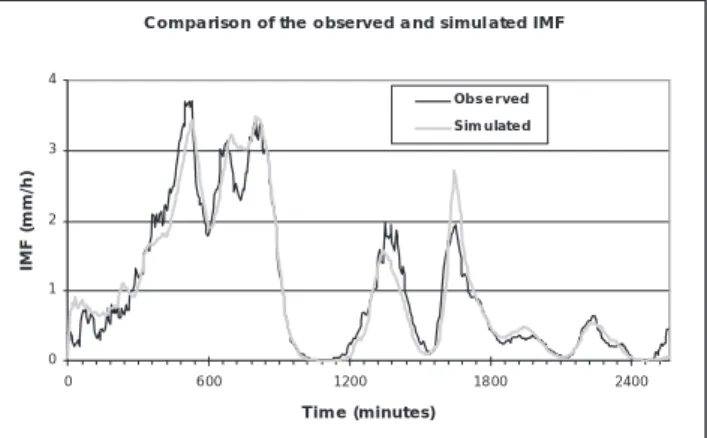
C o m p a riso n o f th e o b se rve d a n d sim ul a te d IM F
0 1 2 3 4 0 6 00 1200 18 00 2400 T im e (m in u te s) IM F ( m m /h) Ob s e r ve d Sim u la te d
Fig. 7. A sequence of corresponding pairs of observed (upper row) and simulated (lower row) images formed by aggregating over time
intervals from 15 to 240 minutes and simultaneously over areas from 1 to 16 km square. These aggregations were selected from corresponding intervals in the two sequences, the longer time intervals subsuming the shorter.
Fig. 8. The trajectories of the IMF calculated from the observed
simulated, non-advected image sequence, showing the remarkable amount of bias in the estimation of this (nearly non-stationary) process when compared to its driver function. The other two are the correlogram of the observed advected images at the pixel scale and at the image scale. Other observations on the implications of Fig. 6 can be made. The first is the difference between the PSI correlograms of the advected and non-advected images at the pixel scale; the latter has considerably more correlation than the former, due only to advection, as expected. Second, the driver function matches the image scale correlogram closely at short lags, a feature which is needed for maintaining a reasonable short-term correlation, but drops off at large lags more rapidly, or else the small-scale structure is too persistent. The images and discussion which follow justify the approach adopted here for validating the model.
A set of observed and their corresponding (in time) simulated images is shown in Fig. 7. These are accumulated over a range of space and time scales; the longer intervals subsume the shorter, hence the similarity from pair to pair. Figure 8 shows the IMF time history for both the observed and simulated sequences. The differences are due to the fact that the statistics of the individual images relate to the underlying continuously varying distribution, whereas the sampling is done on integers; in addition, the mask will have an unbiased (Pegram and Clothier, 2001) but noisy resampling influence on the advecting fields.
The simulations are satisfactory in appearance and the IMF sequence has been well reproduced as expected. It remains to examine the downscaling behaviour of the model statistically.
Aggregation of the Images for the
Purpose of Comparing Downscaling
Behaviour
The statistics of interest here with respect to rainfall intensities are:
l the marginal distribution
l the spatial correlation as measured by the spectrum
l the serial correlation as measured by the correlogram
for aggregations in space and time.
The aggregations will be made spatially over squares of side
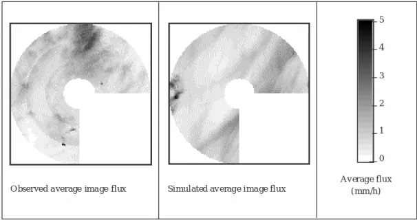
O bser ved a ver age ima ge flux Simu lated av erag e ima ge flu x
Av er ag e flu x ( mm /h ) 5 4 3 2 1 0
Fig. 9. The PSI averaged over the 512 images making up the observed and simulated sequences
S u rvivo r fu n ctio n s o f sa m p l e d a v e ra g e P S I o ve r o b se rve d a n d sim u la te d se q u e n c e s o f 512 im a g e s 0.00 01 0.0 01 0.01 0.1 1 0.1 1 10 P S I (m m /h r) E x c e e de nc e pr oba bi li ty s im u lat e d o bs e r ve d
Fig. 10. A comparison of the survivor functions of the PSI values
from 1 km to 16 km and temporally from 15 minutes to 6 hours. To help increase the number of samples for the larger aggregations (the images are 128 km square and they span 42 hours) the assumption of ergodicity is made, without checking.
The first image is of the average PSI accumulated over the observed and simulated 42-hour event, shown in Fig. 9, where it is seen that the main features, although distributed differently, have been maintained by the simulation. The rings in the observed image are artefacts of the projection algorithm used for converting volume-scan radar reflectivities to rain-rate at a constant altitude. This artefact in the measured image, of course absent from the simulated image, tends to obscure the streakiness due to advection in the former, so clearly seen in the latter. The marginal distributions of the two images are presented in Fig. 10 as survivor functions.
Noting that Fig. 10 is plotted to a logarithmic scale, the match for the accumulations over the full 42 hour period is remarkably good, especially up to 5% exceedence probability. Deviation beyond the 5% could be due to a variety of reasons, the most likely of which is that this is the comparison of only one simulation with its historical counterpart. It is possible that the two parameter log-normal distribution is an imperfect descriptor of the marginal distribution of rainfall intensities, particularly at the higher intensities. A gamma distribution or a truncated log-normal distribution may be a better model, but the possibility was not pursued in this study The remaining figures will explore the intermediate space and time scales.
Figure 11 shows the spatially averaged power spectra for chosen pairs of observed and simulated images with PSI accumulated over 15, 30, 60, 120 and 240 minutes and averaged over squares with sides 1, 2, 4, 8 and 16 km shown
in Fig. 7. The correspondence between observed and simulated spectra is again very good, only starting to wander away from each other at the 16 km/240 minute scales where there are very few sample points. Although the spectra flatten at low frequencies, they can each be defined
satisfactorily by a single parameter, βspace . This economical
representation will be exploited in Fig. 12 when making more general comparisons of the spatial behaviour of the observed and simulated image sequences.
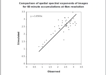
Figures 12a and b show the relationship between βspace
computed for observed and simulated images accumulated over matching times. Figure 12a is for 15-minute accumulations at 1 km resolution, while Fig. 12b is for 60-minute accumulations at 4 km resolution. Longer times and larger areas reduce the number of samples, and the scatter worsens, so the figures are not instructive. The conclusion
Co m p a ri so n o f sp a tia l sp e ctra l e x p o n e n ts o f im a g e s fo r 60 m in u te a ccu m u la tio n s a t 4km re so lu tio n
y = 1.0 503x 0 0.5 1 1.5 2 2.5 3 3.5 0 0.5 1 1.5 2 2.5 3 3.5 O b se rve d Si m u la te d Co m p a ri so n o f sp a tia l sp e ctra l e x p o n e n ts o f im a g e s fo r 15 m in u te a ccu m u la tio n s a t 1k m re so lu tio n
y = 1.0556x 0 0.5 1 1.5 2 2.5 3 3.5 0 0.5 1 1.5 2 2.5 3 3.5 O bs e r ve d Si m u la te d
Spectra of observe d and simula ted data a t various spatially avera ged and temporally accumulated sca les
1 10 100 Wave num be r (k m-1) S p e c tr a l d e n s it y 1km, 15 minute 2km, 30 minute 4km, 60 minute 8km, 120 minute 16km, 240 minute 1/15 simulated 2/30 simulated 4/60 simulated 8/120 simulated 16/240 simulated 10 103 105 107 109 S p ec tra l D en sit y Wave number (km-1)
Radially averaged power spectra for real and simulated space-time aggregations
Fig. 11. The radially averaged power spectra calculated from the
upper row of observed images of Fig. 7 (symbols) with those fitted to the lower row of simulated images of Fig. 7 (lines).
Fig. 12a. Scatter plot of pairs of b values computed for concurrent
pairs of images in the observed and simulated sequences, accumu-lated over 15 minutes
Fig. 12b. As for Fig.12a but for 60 minute accumulations over 4 km
drawn from Fig.12 is that there is, on average, fair correspondence with little bias between the spatial correlations of accumulations of PSI over space and time, between the simulated and observed sequences, as measured by the spectra.
Turning finally to temporal correlation, the spectrum is
no longer described satisfactorily by a power-law relationship because it flattens at both high and low frequencies. The procedure adopted here was not to align the sequences for comparison purposes but to compute the serial correlations for accumulations over 15, 60 and 124 minutes and spatial averages over 1, 8, 32 and 128 km squares, directly from the observed and simulated sequences, which both have the same advection history.
These correlograms are shown in Figs. 13a, b and c, those for the observed sequences given by lines and those of the simulated sequences by markers. In all three cases, there is excellent correspondence at the 128 km (image) scale, as expected, since the model is driven by statistics which are measured at this scale. The correlations of the simulated sequences tend to be smaller than the corresponding observed values and the correlation length compares reasonably well. Generally speaking, the correlation of aggregations in time have been captured remarkably well by the model.
Conclusion
The String of Beads model of space-time rainfields was presented in time series mode. This formulation exploits a time series description of the image mean flux (IMF) using an AR model upon which the space-time statistics are conditioned. The pixel scale intensity (PSI) process is modelled by a second time series also of AR type which is a driver to ensure proper pixel to pixel dependence in time. The spatial correlation is defined by one parameter, the exponent of the power-law fitted to the two-dimensional spatial spectrum of each image. This ensures the proper distribution of variance between the image and pixel scales. Because of the time series structure driving the development of the model’s images in time, it is a model which can be used for simulation and now-casting. In this paper, however, it was used to mimic statistically an observed 42-hour rainfall event.
Each image of the event was shown to be defined by three
statistics, σ, µ and βspace , and the time series of these image
statistics were extracted from the data. The advection of the observed event was captured in its cumulative advection vector. The simulated event was then given the same image statistics and advection vector as the observed event and a parallel set of rainfield images was generated.
The images of the simulated and observed events were compared by aggregating the PSIs over several intervals of time and space. Spatial comparisons were made by exploiting the parsimonious description of the spatial correlation structure via the exponent of the power-law approximation to the spatial power spectrum of each set of C o m p a r i tiv e a u toc o r re l a ti on fu nc ti o ns fo r 24 0 m in u te a ccu m u la tio n s
a t va r io us sp a ti a l r e so lu tio n s 0 0.2 0.4 0.6 0.8 1 0 180 360 540 720 L a g (m in u te s ) O bs erv ed 1km S imulated 1km O bs erv ed 8km S imulated 8km O bs erv ed 32km S imulated 32km O bs erv ed 128km S imulated 128km
Co m p a r i ti v e a u to c o rre l a ti o n fu ncti o n s fo r 1 5m i n ute a cc u m ul a ti o n s a t va r i o us sp a tia l r e so l u ti o ns 0 0.2 0.4 0.6 0.8 1 0 180 360 540 720 L a g ( m in u t e s ) O bs erv ed 1km Simulate d 1km O bs erv ed 8km Simulate d 8km O bs erv ed 32km Simulate d 32km O bs erv ed 128km Simulate d 128 km
C o m pa r iti v e a uto c or r e l a tio n fun c ti on s fo r 6 0 m i nu te a cc um u l a ti on s a t va rio u s sp a ti a l r e so lu tio ns 0 0.2 0.4 0.6 0.8 1 0 180 360 540 720 L a g (m i n u te s ) O bs er v ed 1km S imulated 1km O bs er v ed 8km S imulated 8km O bs er v ed 32km S imulated 32km O bs er v ed 128km S imulated 128km
Fig. 13a. Serial correlograms of accumulations over 15 minutes of PSI over areas up to image scale for both observed and simulated sequences, the former in markers and the latter in lines.
Fig. 13b. As for Fig.13a but for 60 minute accumulations
temporal aggregation. The match of corresponding sets of data was seen to be excellent, even up to the aggregation of the 42-hour events. The temporal correlation structure of the aggregations is good at the image scale, as would be expected, but drops off slightly as the aggregation area reduces. The remedy is to modify the correlogram of the driver of the PSI time series model to have more correlation at small lags which is accomplished in an iterative fitting process. Finally, the String of Beads model has been shown to downscale well in space and time and also to aggregate well over a 42-hour period. It continues to show promise as an operational, high resolution, space-time model of rainfields.
Acknowledgements
The work reported here was funded by a contract between the Water Research Commission of South Africa and the University of Natal, providing full support for the second author, which is gratefully acknowledged. The encourage-ment and support of the steering committee, in particular its chairman George Green, is acknowledged with pleasure. The assistance of the Precipitation Research Directorate of the South African Weather Bureau in the provision and interpretation of the radar data and, in particular, the continued support of Deon Terblanche, is much appreciated and acknowledged.
References
Bell, T.L., 1987. A space-time stochastic model of rainfall for satellite remote sensing studies, J. Geophys. Res., 92, 9631– 9643.
Box, G.E.P. and Jenkins, G.M., 1970. Time Series Analysis:
Forecasting and Control. Holden Day, San Francisco
Cox, D.R. and Miller, H.D., 1972. The Theory of Stochastic
Processes. Chapman and Hall, London.
Crane, R.K., 1990. Space-time structure of rain rate fields. J.
Geophys. Res., 95, 2011–2020.
Cressie, N.A.C., 1991. Statistics for Spatial Data. Wiley, Chichester, U.K..
Foufoula-Georgiou, E. and Krajewski, W., 1995. Recent advances in rainfall modelling, estimation and forecasting. Rev. Geophys. July Supplement, 1125–1137.
Marsan, D., Schertzer, D. and Lovejoy, S., 1996. Causal space-time multifractal processes: predictability and forecasting rain fields, J. Geophys. Res., 101, 26333–26346.
Menabde, M., Harris, D., Seed, A.W. and Austin, G., 1997. Self-similar random fields and rainfall simulation. J. Geophys. Res. 102, 13509–13515.
Mittermaier, M.P. and Terblanche, D.E., 1997. Converting weather radar data into Cartesian space: a new approach using DISPLACE averaging. Water SA, 23, 46–50.
Pegram, G.G.S. and Clothier, A.N., 1999a. High resolution
space-time modelling of rainfall: the “String of Beads” model. WRC
Report No. 752/1/99 to the Water Research Commission, Pretoria, South Africa.
Pegram, G.G.S. and Clothier, A.N., 1999b. The String of Beads rainfall model and its application in simulation and forecasting.
Proceedings 9th SA National Hydrology Symposium, University
of the Western Cape, South Africa.
Pegram, G.G.S. and Clothier, A.N., 2001. High resolution space– time modelling of rainfall: the “String of Beads” model, J.
Hydrol., 241, 26–41.
Pegram, G.G.S. and Seed, A.W., 1998. The Feasibility of
Stochastically Modelling the Spatial and Temporal Distribution of Rainfields. WRC Report No. 550/1/98. to the Water Research
Commission, Pretoria, South Africa.
Schertzer, D. and Lovejoy, S., 1987. Physical modelling and analysis of rain and clouds by anisotropic scaling multiplicative processes. J. Geophys. Res., 92, 9693–9714.
Seed, A.W., Srikanthan, R. and Menabde, M., 2001. A space and time model for design storm rainfall. J. Geophys.Res., 9693–
9714.
Taylor, G.I., 1938. The spectrum of turbulence. Proc. Roy. Soc.
Lond., A, 164, 476–490.
Zucchini, W.S. and MacDonald, I.L., 1999. Illustrations of the use of pseudo-residuals in assessing the fit of a model. Proc.14th
International Workshop on Statistical Modelling, H. Friedl, A.