Econometric Analysis of the Relationship between
Accessibility and Housing Price
by
Gary Yau
Bachelor of Science Engineering ( Electrical Engineering) University of Michigan, Ann Arbor, 1994
Submitted to the Department of Urban Studies and Planning in Partial Fulfillment of the Requirements for the Degree of
Master in City Planning at the
Massachusetts Institute of Technology February 1998
© 1998 Gary Yau
All rights reserved
The author hereby grants to MIT permission to reproduce and to distribute publicly paper and electronic copies of this thesis document in whole or in part.
Signature of Author ...
Certified by ...
Accepted by ...
... . . . . . . . : . . . . . . . . . . . . . . . . . . . .
Department of Urban Studies and Planning January 15, 1998
Qing Shen Mitsui Assistant Professor of Urban Studies and Planning Thesis Supervisor
. . . .. . . . .. . . .. . . .. . . . .. . .
Lawrence Bacow Professor of Law and Environmental Policy Chair, Master in City Planning CommitteemAR 23199,
Econometric Analysis of the Relationship between
Accessibility and Housing Price
by
Gary Yau
Submitted to the Department of Urban Studies and Planing on January 15, 1998 in Partial Fulfillment of the Requirements for the Degree of Master in City Planning
Abstract
Accessibility is one of the major determinants of housing price. To model housing
price, many urban researchers have adopted the method of hedonic analysis. The main question addressed in this paper is: Are the existing hedonic price models adequate in capturing the effect of accessibility? In most of these models, accessibility is represented by rather simplistic measures, such as "distance-to-CBD" and "distance-to-subcenters". The purpose of this research is to explore alternative measures of accessibility that are more sophisticated, and to construct improved hedonic models by incorporating the new measures.
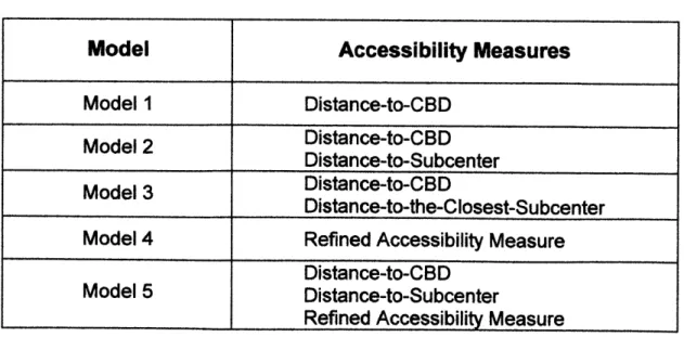
Five models were developed in this research, using a sample of housing transaction data in the Boston Metropolitan Area. Model 1 uses the traditional "distance-to-CBD" as the accessibility measure. Model 2 adopts the subcenter notion of polycentric cities, in which the "distance-to-subcenters" is used in addition to "distance-to-CBD" in modeling housing price. Model 3 explores the impact of the "distance-to-the-closest-subcenters" on housing price. Model 4
incorporates a more sophisticated measure of accessibility that includes the spatial pattern of demand and supply of employment opportunities. Model 5 adds to the 4th model with distances to subcenters. Regression results indicated that the model 5, which combines both the "distance-to-subcenters" and the refined
accessibility measure, performed best.
Geographic Information System (GIS) plays an important role in this research. From data handling and model building, to subcenter identification and distance calculation, GIS was used intensively. GIS is critical to the success of this research.
Thesis Supervisor: Qing Shen
Acknowledgments
I deeply appreciate my thesis advisor, Professor Qing Shen, for his invaluable
guidance throughout the writing of my thesis. I would also like to thank my thesis reader, Professor William Wheaton, for his comments and suggestions. Words are not adequate to express my gratitude to them.
I would also like to express my appreciation to my friends, Chi-Fan Yung, Akemi
Yao, Sylvia Wey, Ming Zhang, Christine Tse, and Hiroshi Tamada. They not only helped shape many of the ideas in this thesis, but also provided emotional
support throughout my stay at MIT.
Most of all, I would like to thank my parents for their support and encouragement, and for their love and understanding for so many years.
Gary Yau
Table of Contents
Abstract ...
2A cknow ledgm ent
...
3
1. Intro d u ctio n
...
8
1.1 Research Background 1.2 Research Questions
1.3 Thesis Organization
2. Literature Review and Model Development ... 14
2.1 Hedonic Housing Price Model 2.2 Employment Accessibility Measure
2.2.1 Hansen Type Measures 2.2.2 Refined Accessibility Measure
2.2.3 Refined Accessibility Measure with 2 Transportation Modes
3. Research Methodology
...
243.1 Housing Price Model
3.2 Hedonic Housing Price Analysis Method
3.2.1 Model Development
3.2.2 Housing Price Determinants 3.2.3 Data Source
3.2.4 Procedure of Hedonic Analysis
3.3 Distance to Subcenters Measure
3.3.1 Identification of Subcenters
3.3.2 Procedure for Subcenter Identification
3.3.3 Procedure for Calculating Distance-to-Subcenter
3.4 Refined Employment Accessibility Measure
3.4.1 Refined Accessibility Measure with 2 Transportation Modes 3.4.2 Data Source
4. Results of Hedonic Housing Price Model ... 51
4.1 Model 1 - Monocentric Model
Description of Result Interpretation and Analysis
4.2 Model 2 - Polycentric Model, with
Subcenter Measure 4.2.1
4.2.2
Distance-to-Specific-Description of Result
Interpretation and Analysis
4.3 Model 3 - Polycentric Model, with
Subcenter Measure 4.3.1
4.3.2
Distance-to-the-Closest-Description of Result
Interpretation and Analysis
4.4 Model 4 - Refined Accessibility Measure Model
4.4.1
4.4.2 Interpretation and AnalysisDescription of Result
4.5 Model 5 - Polycentric with Refined Accessibility Model 4.5.1
4.5.2 Description of ResultInterpretation and Analysis
5. Conclusion
...
89
5.1 Summary of Research Findings
5.2 Future Research
A p p e n d ix
...
92
Appendix A. Appendix B. Appendix C. Descriptive StatisticsCorrelation Coefficient Matrix Important Arc/Info Commands
B ib lio g ra p hy
...
954.1.1 4.1.2
List of Figures
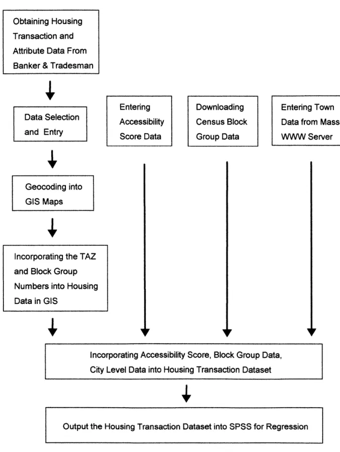
Figure 3.1 Location of Housing Transaction Cases Figure 3.2 Towns and TAZ zones in Boston MSA Figure 3.3 Procedures of Hedonic Regression Analysis Figure 3.4 Employment DensityFigure 3.5 Spatial Relationship of Housing Transaction Cases and Subcenters Figure 3.6 Data Sources of Accessibility Calculation
Figure 3.7 Procedure of Accessibility Calculation
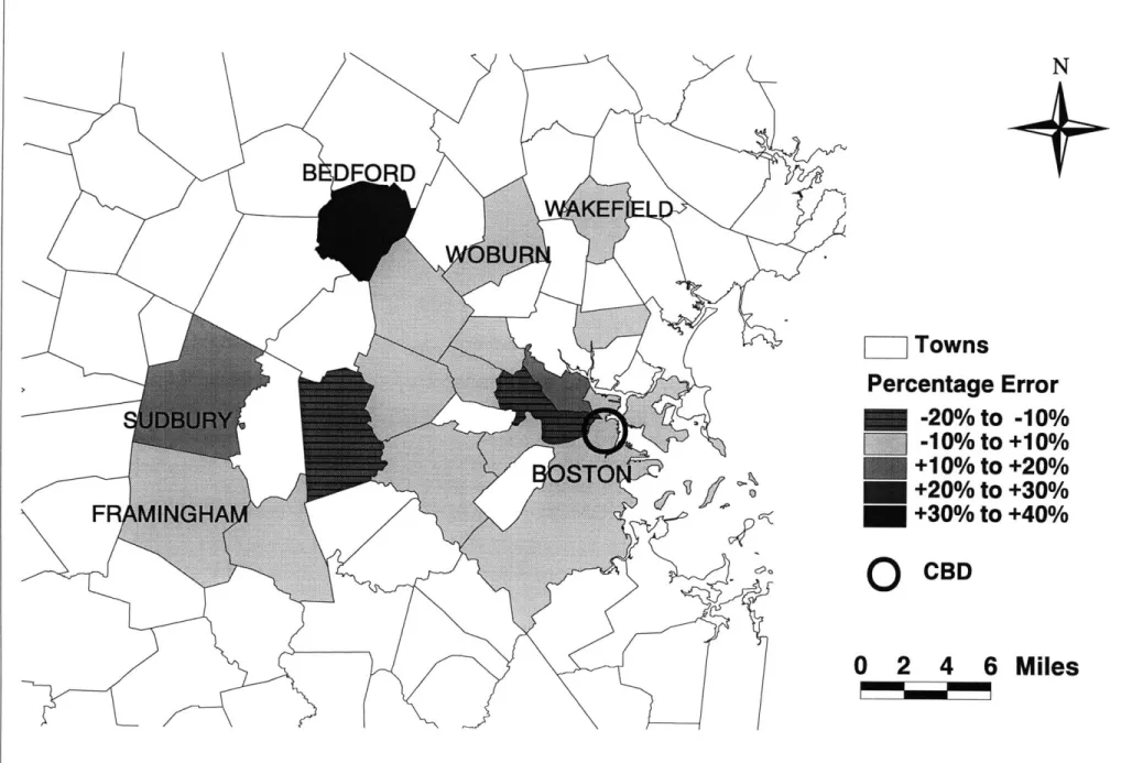
Figure 4.1 Predicted Price vs. Observed Price of Model 1 Figure 4.2 Average Percentage Error Distribution of Model 1 Figure 4.3 Predicted Price vs. Observed Price of Model 2A Figure 4.4 Average Percentage Error Distribution of Model 2A Figure 4.5 Predicted Price vs. Observed Price of Model 2B Figure 4.6 Average Percentage Error Distribution of Model 2B Figure 4.7 Predicted Price vs. Observed Price of Model 3 Figure 4.8 Average Percentage Error Distribution of Model 3 Figure 4.9 Predicted Price vs. Observed Price of Model 4 Figure 4.10 Average Percentage Error Distribution of Model 4 Figure 4.11 Predicted Price vs. Observed Price of Model 5A Figure 4.12 Average Percentage Error Distribution of Model 5A Figure 4.13 Predicted Price vs. Observed Price of Model 5B Figure 4.14 Average Percentage Error Distribution of Model 5B
List of
Tables
Table Table Table Table Table Table 3.1 4.1 4.2 4.3 4.4 4.5 Table 4.6 Table 4.7 Table 4.8 Table Table Table Table Table Table Table Table Table 4.9 4.10 4.11 4.12 4.13 4.14 4.15 4.16 4.17Housing Price Determinants
Accessibility Measures in the 5 Models Regression Result of Model 1
Percentage Impact of Distance-to-CBD on Housing Price at 2 Mile Increment
Percentage Impact on Housing Price at Each Additional Bathroom Percentage Impact on Housing Price at Each 1,000 Square Feet
Increase of Lot Size
Percentage Impact on Housing Price at Each 1,000 Square Feet Increase of Living Area
Percentage Impact on Housing Price at Each $10,000 Increase in Median Household Income
Percentage Impact on Housing Price at Each 10% Increase in the Percentage of Block Group Resident Having College Degree Regression Result of Model 2A
Excluded Variables in Model 2A Regression Result of Model 2B
Percentage Impact of Distance-to-Subcenters on Housing Price at 2 mile Increments
Regression Result of Model 3 Regression Result of Model 4 Regression Result of Model 5A Excluded Variables in Model 5A Regression Result of Model 5B
1
Introduction
1.1 Research Background
Court (1939) and later Griliches (1971) pioneered hedonic analysis techniques to model housing price with real housing transaction data. Many housing price models with various identified housing price determinants have been developed since the 70's following the hedonic approach. Along with other housing price determinants such as housing attributes and community characteristics,
accessibility has been recognized as having significant impact on housing price. Earlier monocentric models emphasized on employment accessibility to the Central Business District (CBD), the only employment center ( Alonso(1 964).
Mills(1 967), and Muth(1 969) ). It is believed that there exists a housing price gradient from the CBD to the boundary of the metropolitan area. The distance-to-CBD was used as the accessibility proxy in the hedonic analysis. However, the emergence of employment subcenters observed in the last few decades in many metropolitan areas has shown a gradual shift in urban system from monocentric city to polycentric city. This decentralization trend has undermined the
appropriateness of monocentric city housing price gradient model.
To capture the impact of decentralization in housing price modeling, several hedonic models (Landsberger and Lidgi, 1978; Romanos, 1977; Greene, 1980; Getis, 1983, Erickson, 1986; Gordon et al, 1988; Peiser, 1987; Heikkila et al,
1989; McDonald and McMillen, 1990; Waddell et. al, 1993) that take employment
subcenters into consideration were developed since the 1980's. The researchers selected several employment subcenters in the metropolitan region. Distances from the housing units to the subcenters were then calculated. The researchers then incorporated the distance-to-subcenter measurements, along with other housing attributes and community characteristics, into the hedonic regression analysis. Finally past housing transaction data were entered into the regression analysis to estimate the coefficients of the housing price determinants.
However, the distance-to-subcenter measure, though superior to traditional CBD price gradient model, sheds no light on the reason why proximity to the
subcenters is valued by people. Since the subcenters were often chosen based on their large employment opportunities, many researchers regarded the
distance-to-subcenter as the employment accessibility measure. The
appropriateness of using distance-to-subcenter as employment accessibility proxy is questionable for several reasons.
First, even though subcenters represent significant portion of employment opportunities, there exist many other employment opportunities in areas not
identified as employment subcenters. These employment opportunities are not captured in these models. Moreover, without considering the number of jobs in subcenters as well as the number of people in labor force, the "distance-to-subcenters" considered the employment opportunities in subcenters as public goods, which is flawed. Furthermore, in additional to job opportunities, subcenters also offer a wide range of services and amenities. These services and amenities are also valued by people and thus are believed to have impact on housing price. These impacts, however, can not be separated from the impact of job
opportunities in the distance-to-subcenter measure. For the above reasons, the significance of employment accessibility tends to be misrepresented in the distance-to-subcenter measure in the hedonic housing price analysis.
To accomplish the goal of developing a model that captures the significance of employment accessibility, this research proposes to incorporate a refined employment accessibility measure into the hedonic regression analysis.
There has been significant development in the employment accessibility measure since the Gravity-Type measurement was proposed in 1959 (Hansen, 1959). This model was further modified by Weibull (1976) and later by Shen (1996) and
myself to incorporate job competition by different modes of transportation. This employment accessibility measure takes into consideration of every single jobs in the area, the travel time to these employment opportunities, and also the
competing demand from the area for the jobs.
With the advance in the Geographic Information System (GIS) technology, many of the data manipulation, computation, spatial analysis, and visualization involved in this research that were once either labor-intensive or impossible are made possible today. With the help of GIS, I intend to incorporate this new employment accessibility measure into the hedonic housing price model in this research, using Boston as the case under study. This refined employment accessibility measure provides a potentially better means to evaluate the impact of accessibility on housing price. It also sheds light on several other research questions that will be discussed in details in section 1.2.
1.2
Research Questions
This research is intended to explore the answers to the following research questions:
I. Does proximity to CBD have significant impact on housing price in Boston Metropolitan Area?
The first part of this research follows the methodology of early monocentric housing price model which incorporates the distance-to-CBD into the regression analysis. The regression results will show whether the distance to Boston CBD does have significant impact on housing price.
2. Does the polycentric model do better than monocentric model in housing price modeling in Boston MSA? Does the distance-to-subcenter have significant impact on housing price?
This research will also attempt to adopt the polycentric housing price model. Prior study has shown that polycentric model does better than monocentric model in housing price modeling. This research will apply the model to Boston MSA, which has shown a continuing trend of
decentralization, to explore if polycentric model does perform better than traditional monocentric model.
3. If the subcenters do have impact on housing price, which
subcenters are they? the closest subcenters? or certain particular subcenters?
The polycentric model was adopted by earlier researchers on the assumption that distance-to-subcenter has impact on housing price. However, in most of the prior studies, distance to "specific" subcenter was used. For example, the distance to subcenter X was calculated for each case of housing data and entered into the regression analysis. The
question of whether the distance to the "closest" subcenter has impact on housing price was left unanswered. This research will also try to
answer this question.
The traditional distance-to-subcenter measure tends to misrepresent the employment accessibility. The improved accessibility measure is expected to better capture the true employment accessibility potential, and thus this research is expected to shed new light on this well-studied research question.
5. How do the employment accessibility by driving and by transit differ in their impact on housing price?
The improved employment accessibility measure is able to calculate separately the employment accessibility by different transportation modes. This research will look into the impact of automobile employment
accessibility and public transit employment accessibility on housing price.
6. Do proximity to CBD and proximity to subcenters have impact on housing price, for reasons other than the employment opportunities offered by CBD and subcenters?
This research will also try to analyze if there exists housing price gradient in the CBD and in the subcenters due to factors other than employment, by incorporating both the distance-to-subcenter measure and the modified employment accessibility measure into the regression analysis. By doing so, the impact of employment accessibility on housing price will be accounted for by the accessibility measure. Thus, the impact of other
attractions in the CBD and subcenters on housing price will be revealed by the coefficients and t-scores of the CBD and the distance-to-subcenter variables in the regression analysis.
Details on how these research questions are answered are discussed in detail in Chapter 2 "Literature Review and Model Development" and Chapter 3 "Research Methodology".
1.3 Thesis Organization
The thesis consists of 5 chapters, as discussed below.
Chapter 1 introduces the background and the purpose of this research. The research questions, contribution of this research, and the organization of the thesis are also presented.
Chapter 2 explores theories and earlier studies relevant to this research. The literature review of the hedonic housing price analysis and employment
accessibility measures are presented. The development of the models adopted in this research is also discussed.
Chapter 3 brings the attention back to the methodology and the procedure of this study. The 5 different models that were used in this research are introduced, followed by the discussion of the methodology and the procedures of hedonic
housing price analysis, subcenter identification, and employment accessibility calculation.
Chapter 4 presents the modeling results of the 5 hedonic housing models. The analysis and interpretation of the results are thereafter discussed.
Chapter 5 concludes the thesis with a summary of the findings of this research. Future research possibilities are also explored.
2
Literature Review and Model Development
Literature review and development of housing price models as well as
accessibility measures are presented in this chapter. In Section 2.1, the housing price model that employs the hedonic technique is presented and analyzed. The hedonic technique is used in this research with past housing transaction data to build the housing price model.
Most of prior hedonic housing price models adopted some kind of accessibility measures in the regression analysis, as it is generally accepted that housing price is influenced by the housing location, specifically, the accessibility of the house to desired locations and amenities. In section 2.2, the evolution of accessibility
measure will be discussed in detail. Special attention is paid to the accessibility of employment. Different employment accessibility measures are analyzed and compared. A refined measure that takes employment competition into
consideration is developed and to be included in the hedonic regression analysis. It is believed that accessibility to employment opportunities has strong influence on housing price.
2.1
Hedonic Housing Price Model
In housing market, the land and housing are often referred to as completely product-differentiated because each product sold in the market is unique
(DiPasquale and Wheaton 1996). Purchasing a "product" in this market is viewed as purchasing a bundle of "attributes" (Lancaster 1966). For example, each house comes with different lot size, living area, number of bathrooms, number of bedrooms, structure, age, design of house, neighborhood, pollution, police protection, and location to employment opportunities, etc.. Each of these attributes carries certain value, or in other words, price tag. To put it in a very simple way, the weighted sum of all the "price tags" of the attributes is the market price of a housing unit (Griliches, 1971).
Due to this "bundle of attributes" characteristics of housing price, a good way to model housing price would be to determine the value of each of these attributes, and the sum of these values would be the price of a housing unit. Court (1939) and later Griliches (1971) pioneered hedonic price analysis techniques to model housing price using multiple regression analysis with real transaction housing price as the dependent variable, and housing attributes as the dependent
variables. With regression analysis, the "price tag" of each of the major attributes, or price determinants, can be estimated with real housing transaction data.
Models can therefore be built to predict and assess housing price based on the estimated price tags of housing attributes.
There has been enormous interest in empirical hedonic housing price analysis in the last 2 decades. In his 1982 paper, Miller (1982) classified the housing price determinants into 5 major categories: physical attributes, location, financial
factors, transaction costs, and inflation. Since there can be millions of factors that affect the price of a housing unit, these researchers tend to incorporate most of the known and tested major price determinants, and then focus the research on a less known price determinant or an improved measure of a known price
determinant.
Among these studies, accessibility has continued to be a major focus of research interest. Earlier research focused on the employment accessibility, typically
measured by the distance from the house location to CBD. These studies generally confirmed the existence of price gradient from the CBD out (Alonso 1964, Mills 1972, Muth 1969). In other words, the closer the house to CBD, the higher the price. However, the emergence of employment subcenters observed in last few decades in many metropolitan areas has shown a gradual shift of urban system from monocentric city to polycentric city. Many recent researchers have incorporated distance-to-subcenter into the hedonic housing price model with modest success (Landsberger and Lidgi, 1978; Romanos, 1977; Greene, 1980; Getis, 1983, Erickson, 1986; Gordon et al, 1988; Peiser, 1987; Heikkila et al,
1989; McDonald and McMillen, 1990; Waddell et. al., 1993). Among these
researchers, Heikkila et. al. concluded that the price gradient from the CBD is statistically insignificant in the case of Los Angeles.
The accessibility measure used in most of these researches are simply the straight line distance from the location of the house to the CBD. Some researchers used travel time, instead of "fly" distance, as the proxy of
accessibility (Kain and Quigley 1970; Lapham 1971; Rothenberg et.al., 1991). Yet some other researchers used a variety of accessibility measures such as number of block units to the CBD, miles of bus lines or number of stations in a neighborhood, and straight line distance to employment centers weighted by the size of each center.
Many of these researchers used the term "employment accessibility" to describe the straight line distance to these subeenters, as these subcenters are often
identified by their high employment opportunities. This raises the question of what exactly the "distance-to-subcenter" represents. These centers often offer services and amenities other than simply employment opportunities. The distance
measure makes no distinction between job opportunities and other services and amenities, and thus the conclusions of these research that employment
Another possible loophole in the conclusion that employment accessibility matters is that even though these employment subcenters represent a large portion of total employment opportunities in the region, many other local employment opportunities were not accounted for. And thus the significance of employment accessibility is misrepresented in the distance-to-subcenter measure. The conclusion that employment accessibility matters is again questionable.
Yet another potential problem with the distance-to-subcenter measure is that it does not consider the demand and supply of job opportunities. Some researchers weighed the distance by the size of the subcenters. However, the weighed
distance considered only the supply side of employment, the demand side of employment was not taken into consideration. Without considering the demand
side of the employment market, the employment opportunities are implicitly
treated as public goods. Whether the supply side of the employment opportunities can fully represent the whole employment potential of an area is questionable. This research is intended to look into this problem by incorporating an
accessibility measure that takes into consideration all job opportunities in the Metropolitan Area. What is more significant about this accessibility measure is that it also takes into consideration the employment competition. Details of the accessibility measure is discussed in section 2.2. This research will try to answer the research question of whether employment accessibility really matters, and whether this new measure does better in predicting housing price than the traditional straight line distance measure.
Given the new accessibility measure, it is now also possible to answer the research question of whether the distance-to-subcenter still has impact on
housing price after all the employment opportunities have been accounted for by the new accessibility measure. This can be done by incorporating both the
distance-to-subcenter and the new accessibility measures into hedonic regression analysis. The statistical significance of the distance-to-subcenter
variable can be an indication of whether the amenities provided in these
subcenters have impact on housing price, and the coefficient will show how large this impact is.
2.2
Employment Accessibility Measure
The literature review and model development of the employment accessibility measures that were incorporated into the housing price model are presented in this section. In section 2.2.1, the traditional Hansen Accessibility measurement is presented. Section 2.2.2 discusses a refined model that takes into consideration of both demand and supply of employment opportunities. In section 2.2.3, two different modes of transportation are incorporated into the refined accessibility measure. This measure is to be used in the hedonic housing price regression analysis.
2.2.1
Hansen Type Measures
Accessibility denotes the ease with which spatially distributed opportunities may be reached from a given location using a particular transportation mode (Morris, Dumble, and Wigan, 1979). Hansen (1959), among others, developed the first accessibility measure to quantify accessibility into comparable numeric "scores". This measure, being widely used today, can be generally expressed as:
A i = I0 f(Cij) ... (2.1 )
where
A = Accessibility for zone i
0 = Number of opportunities in location
j
Cj = Travel time, distance, or cost for a trip from zone i to zone
j
f(Cij) = The impedance function measuring the spatial separationbetween zone i and zone
j
i = The zone where the accessibility is being calculated
The travel impedance of the above equation can be in many different forms. The original form is the power function adopted from Newton's Law of Gravity.
Alternative forms of spatial separation impedance include exponential functions (Wilson, 1971). Exponential function with travel time was adopted in this
research: 1 f( C i) ... ( 2.2 ) (0p Cii)
e
whereCij = Travel time from zone i to zone
j
= The parameter for travel impedance,estimated to be 0.1034 (Shen, 1997) for Boston MSA Hansen type accessibility measure has been widely adopted as the accessibility representation. It also has been widely used in urban and transportation planning (Hutchinson, 1974; Meyer and Miller, 1984; Putman, 1983; Wilson, 1974; Shen,
1997).
However, this accessibility measure has a significant limitation in measuring accessibility to employment. A closer look of this measure reveals that it only considers the supply side of employment market. The employment demand, the number of job seekers, is omitted in the equation. The assumption that
employment demand is irrelevant or insignificant in employment accessibility is unfounded. This omission may create biased accessibility measurement, which can be observed in the following example.
The Hansen measure will generate a high accessibility measurement for a zone, if there are a large number of jobs in the zone. However, if there are many more
job seekers than jobs in the zone, the true employmjent potential should be quite
low. The Hansen measure is not able to capture the significance of job competition, and thus the score is not meaningful in this example.
To incorporate employment competition into the calculation of accessibility, a better measure needs to be developed.
2.2.2
Refined Model of Accessibility
A refined accessibility measure was developed by Weibull (1976) and later by
Shen (1997) and myself. To take employment demand into consideration, the number of job seekers has to be incorporated into the accessibility measure. In other words, employment supply has to be discounted by employment demand. To calculate the demand for employment at zone
j,
the number of people in labor force of zone k is multiplied with the travel impedance between zone k and zonej.
The summation of all the demand from each zone to the opportunities in zone
j
is the total demand for employment for zonej.
The demand for employmentopportunity at zone
j
can be written in the following form:Dj = k Lk f( Ckj ) ... (2 .3 )
where
Dj = Demand for employment opportunities at zone
j
Lk = Labor force in zone k
f(CkJ) = The impedance function measuring the spatial separation between zone k and zone j
j
= The zone where the employment opportunities locateSince the true employment accessibility should also reflect the demand for
employment opportunities, the supply of employment should be discounted by the demand. The demand discounted supply takes the following format:
(Sadj)j = = ... (2.4 )
Dj Ek Lk f( Ckj )
In the above equation, the job opportunities available in zone
j
are discounted by the number of job seekers, which is discounted by the relative travel impedance. This demand adjusted supply of employment represents the true employment opportunities of an employment location. To calculate the aggregatedemployment accessibility of every zone to zone i, we can substitute the job
opportunities in equation 2.1 with the discounted job opportunity in equation 2.4 to come up with the refined employment accessibility measure:
O f( Cij)
A4 = Ej ( Sadj)j f( Cij) = j ... (2.5)
Ik Lk f( Ckj )
The above equation depicts the general employment accessibility measure, taking employment demand into consideration. However, people go to work by different transportation modes. Significant difference exist in accessing
employment opportunities by different transportation modes, such as by driving and by taking public transit, and therefore the employment accessibility measure should capture this difference.
2.2.3
Refined Employment Accessibility Measure with
Different Transportation Modes
The difference in accessing employment opportunities by different modes lies in the transportation impedance and auto ownership. The following equation depicts
the refined employment accessibility measure with 2 different transportation modes, auto and public transit.
0 f( Ci; auto)
Aauto = ... (2.6)
E [(k Lk f( Ckj aut*) + ( 1 -ak) Lk f( Ckj tran
Atran = j O f( C,, ran (
Ai"" =... ( 2.7 )
Ek [ak Lk f( C aut ) + ( k
)
Lk f( Ckj tranwhere
A auto = Accessibility by automobile for zone i
Ai tran = Accessibility by transit for zone i
f(Cij auto) = The impedance function measuring the spatial
separation by automobile from zone i to zone j
f(Cij tran) = The impedance function measuring the spatial
separation by public transit from zone i to zone
j
cXk = Automobile ownership of zone k
In the above set of equations, employment accessibility is being calculated based on different modes of transportation. On the demand side, the number of
employment opportunities remains the same for both equations. In this research, travel impedance was calculated based on travel time. It is obvious that the time needed to travel to work differs in different transportation modes, and therefore the different travel time should be used in calculating the travel impedance. On the demand side, the number of employment seekers are further subdivided into those who drive to work and those who take public transit to work. No matter what transportation modes the workers use, their demand potential to an
employment opportunity should always be included in the calculating the total demand potential of the employment opportunity. Therefore the demand side is
the sum of the employment demand by workers using different transportation modes.
With this accessibility measure of the 2 different transportation modes, it is now possible to explore the differences in the impact on housing price by the
accessibility of the 2 different transportation modes. Due to the fact that the majority of US residents drive to work, this research will try to answer the question of whether the employment accessibility by automobile has greater impact on housing price than the employment accessibility by public transit.
3
Research Methodology
Research Methodology is presented in this chapter. In section 3.1, the 5 hedonic models that are developed in this research are presented. Section 3.2 describes the hedonic analysis method adopted in the 5 models. The derivation and
calculation procedure for the distance-to-CBD/Subcenter and refined Accessibility Measure are discussed in section 3.3 and 3.4 respectively.
3.1
Housing
Price Models
Five housing price models are developed in this research. These models are used to analyze the characteristics of accessibility in Boston MSA and its impact on housing price. The different accessibility measures are compared and
analyzed. All of the housing price determinants used in the 5 models are exactly the same, except for the accessibility measures.
Model 1 follows the early monocentric model, in which it is assumed that the CBD is the only employment center in the whole metropolitan area. The distance between the housing unit and the CBD is used as the accessibility measure. Model 2 follows the more recent polycentric model, in which it is assumed that in addition to the CBD, there exist major employment subcenters that also have great impact on housing price. Distance-to-subcenter measures are incorporated
in the hedonic regression analysis to examine if price gradients from these subcenters exist. This model will show how polycentric Boston MSA is, and will also reveal if distance-to-CBD still has impact on housing price after
incorporating employment subcenters.
Model 3 modifies the way in which the "distance-to-subcenter" measure is entered into the hedonic regression analysis. Instead of using the distance from each house to each specific subcenter (such as Framingham, Newton, Waltham, etc.), the distance-to-subcenter in terms of proximity (such as the closest
subcenters, the 2nd closest subcenters, etc.) are entered into the regression
analysis. This model is intended to study whether the distance to the closest subcenter (rather than distance to specific subcenter as in model 2) has impact on housing price.
Model 4 adopts the "refined employment accessibility measure" discussed in Chapter 2 as the only accessibility measure in the hedonic housing price model.
A comparison of model 2 and model 4 will indicate whether the "refined
employment accessibility measure" can do better in housing price prediction than traditional distance measure. In addition, this model reveals the importance and significance of automobile accessibility and transit accessibility in housing price. Model 5 incorporates both "distance to subcenter" and "refined employment accessibility measure" into the hedonic regression analysis. The purpose is to see whether subcenters have impact on housing price for reasons other than employment opportunities.
3.2 Hedonic Housing Price Analysis Method
This section will discuss the development and the use of the hedonic housing price model used in this research. In section 3.2.1, the derivation of the housing
price model used in this research is discussed. The housing price determinants incorporated in the model are presented in section 3.2.2. The data used to
estimate the impact of accessibility on housing price are described and explained in section 3.2.3. Finally, the procedures to run the regression is presented in section 3.2.4.
3.2.1 Model Development
The methodology used in the housing price model development is hedonic regression analysis method, pioneered by Court (1939) and later Griliches
(1971). In Hedonic analysis techniques, the values of independent components
of a heterogeneous good are determined through multiple regression analysis as discussed in Chapter 2.
To determine the housing price, the dependent variable in the hedonic regression analysis, the first thing to do is to identify all the desirable and undesirable features of the house that are believed to have impact on housing price. These features will then be taken as the independent variables in the regression analysis. Market price is generally determined through an ordinary least square multiple regression model, generally in the form of (Miller, 1982):
Housing Price = a + $1X1 + p2X2 + 03X3 + ... + pnXn + 6 Where
X1, X2, ..... . . Xn are the housing and locational features that
affect housing price a is the housing price intercept
$1, 02, ... on are the estimated regression coefficients s is the error of the estimate.
The above regression equation assumes linear correlation between independent variables and dependent variables. Even though linear hedonic equations are frequently used in research and property valuation, they do have the unrealistic assumption that each additional unit of the housing and locational features will add exactly the same additional value to the housing price (DiPasquale and Wheaton, 1996). Due to the law of "diminishing marginal utility", each additional unit of the features should add lesser value to the house than the previous unit. For example, a household may be willing to pay extra $50,000 to bring up the number of bathrooms from 2 to 3, they may only be willing to pay an additional
$30,000 to have 4 bathrooms instead of only 3. This signifies the fact that, in
reality, the assumed linear relationship between housing price and housing price determinants is incorrect.
To capture the law of diminishing marginal utility, a modified regression equation that takes exponential form on the independent variables has been used by many researchers. The following regression equation has "proved superior to linear regression equation" (Miller, 1982; Halvorsen and Pollakowski, 1981):
Housing Price = a X10' X2s2 X3 .. . . .. . .. +
To statistically estimate the parameters in the above equation, we can transform the above equation into a linear equation by taking logarithm on both sides:
Log ( Housing Price) = Log a + 1 log X1 + p2 log X2 + ... + On log Xn
To estimate the coefficients of X1, X2, ... Xn, market value of houses should be
entered into the regression analysis. Since "market value" of houses is not known unless a transaction happens, the best data to be entered into the regression analysis is the actual housing transaction data. In this research, 1064 cases of
1990 single family house transaction data were sought and entered in the
Housing Price Determinants
Many important housing price determinants have been identified in prior studies. In his 1982 paper, Miller summarized prior research results and concluded that the physical attributes of housing units, along with the locational influences, are considered the "fundamental factors" that affect housing price. These features are the most influential housing price determinants and are therefore
incorporated in my study.
To determine the accessibility impact on housing price, the accessibility measures are incorporated into the regression analysis as independent
variables. The accessibility measure used in model 1 is the distance from each housing unit to Boston CBD. For model 2, the measure is the distances from the housing unit to each of the identified subcenters. Model 3 incorporates the distance to the closest subcenters. Model 4 uses the "refined employment accessibility measures" by automobile and by public transit as the accessibility independent variables. Model 5 includes both distance-to-subcenter and the 2 refined accessibility measures used in model 4 as the accessibility independent variables. These accessibility measures are discussed in section 3.3 and section
3.4.
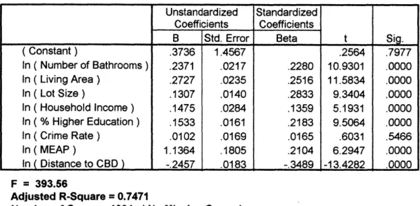
The physical attributes that are used in my research include number of bathrooms, size of living area, and lot size. For community characteristics, I incorporated medium household income, percentage of residents having 4-year college degree, crime rate, and MEAP (Massachusetts Educational Assessment Program) test score. Their expected impacts on the housing price (Miller, 1982) are listed in Table 3.1:
Table 3.1 Housing Price Determinant
3.2.2Housing Price Determinant Impact on Housing Price
Accessibility
Distance to CBD Ne gative
Distance to Subcenter Negative
Employment Accessibility by Auto Positive Employment Accessibility by Transit Positive
Physical Attributes of the House
Number of Bathroom Positive
Living Area Positive
Lot Size Positive
Community Characteristics
Median Household Income Positive
Percentage of College Graduate Positive
Crime Rate Negative
School Quality ( MEAP Score) Positive
3.2.3
Data
To estimate the coefficients of the independent variables, housing values and housing price determinant attributes data must be collected and entered into the regression analysis. For housing price and house attributes, data from Banker and Tradesman, a real estate data company in Boston, were used. For
community characteristics, data from the 1990 Census STF3A file and data from the World Wide Web (WWW) maintained by state government of Massachusetts were used. The details of the data are described below.
1.
Housing Price and Attribute Data
For housing price and housing attributes, 2 sources of data are possible. First, Assessor's Office of each town maintains detailed assessed housing price and housing attributes of each house in the town. However, the housing price in the assessor's file is estimated, rather than the actual market price.
The second source for housing value is past housing transaction data. This type of housing transaction data is usually maintained in the private sector (such as real estate agencies) and does contain the housing market price. However, housing attributes, such as the square footage of the house, may not be included in the housing transaction data.
Based on the shortcomings of both record types, and the demand for detailed housing price data containing transaction price as well as housing attributes, there have been efforts by private companies to combine housing transaction data with assessor's file to come up with a complete housing price database. The housing price and attribute data used in this research are from the combined data "Banker and Tradesman 1990 Annual COMPReport and SALESReport" for Suffolk County and Middlesex County of Massachusetts, published by Banker and Tradesman Real Estate Data Publishing.
Selection and Distribution of Housina Transaction Data
A selection of 1064 transaction data from Boston Metropolitan Area was entered
into the hedonic regression analysis. This data are from the year 1990, and consisted of single family houses only.
The real estate market in the year 1990 was characterized by the large number of foreclosures and auctions. More than 10% of all real estate transaction in 1990 were auctions (Banker and Tradesman, 1990). The auction price is usually much lower than regular market price, and should be omitted in the regression
names of sellers and buyers. By eliminating the transaction data with financial agencies as the seller, the remaining of the data should consist of transactions
under normal market condition.
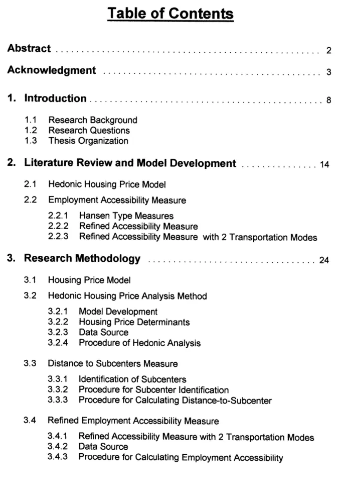
Because of the limitation of data availability, the data were randomly selected from only 16 different towns and cities, including Boston, Cambridge, Somerville, Belmont, Arlington, Bedford, Newton, Weston, Framingham, Lexington, Maiden, Wakefield, Woburn, Natick, Sudbury, and Waltham. These towns and cities cut across a range of towns from the CBD of Boston to Bedford and Framingham on the first circumferential highway ring. Ideally, to have a comprehensive coverage of the study area of Boston MSA, cities from the first circumferential highway to the outer circumferential highway, and to the edge of Boston Metropolitan Area should also be included. Unfortunately, the data provided by Banker and
Tradesman do not contain housing attributes data for towns outside of the first circumferential highway. However, the data on the 16 cities do contain a wide range of locations, housing features, and community characteristics, and therefore the regression results should be meaningful.
2. Community Characteristicscommunity Characteristics were collected from 3 different sources, representing 3 different aggregation levels: TAZ level, block group level, and town level. They are explained below:
TAZ Level
The refined accessibility measures for both automobile and public transit used in model 4 and model 5 were calculated on the TAZ zone level as described in section 3.4. Each of the TAZ zones is composed of 1 or more block group zones.
Figure 3.1 Location of Housing Transaction Cases
.I
0
Towns
Locations
CBD
0
2 4 6
Miles
The community medium household income and the percentage of residents having 4 year college degree used in the regression analysis were collected at block group level from the 1990 US Census STF3A data.
These data are considered better than the town level data described in the next paragraph for the purpose of housing price modeling, because they represent the immediate neighborhood characteristics of the house. Towns are many times larger than block groups and therefore may have areas with significant variation in characteristics. Block group level data should therefore have more consistent influence on housing price.
Town Level
Due to the data availability, several important housing price determinants could only be gathered at the town level. As mentioned in previous paragraph, these data represent an aggregated average across the whole town. Significant variation across the town may exist, and therefore the impact of the town level data on housing price may not be as consistent as the TAZ level data and the block group level data.
The town level data that were incorporated in this research include the crime rate and the MEAP scores (school quality). These data were collected from the World Wide Web server maintained by the state government of Massachusetts.
3.2.4
Procedure for Hedonic Analysis
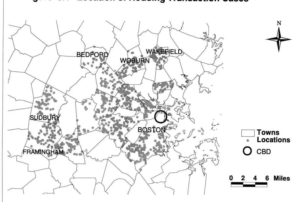
The step by step procedure for the housing price model development is presented in this section. The procedure can be classified in the following 3 major steps: 1. Data Collection and Data Entry, 2. Geo-Coding and Spatial Manipulation, and 3. Regression Analysis. These procedures are discussed in details below, and are illustrated in Figure 3.3.
1.
Data Collection and Data Entry
As mentioned in section 3.2.3, the housing transaction data were taken from the "Banker and Tradesman1 990 Annual COMPReport and SALESReport" for
Suffolk County and Middlesex County of Massachusetts. Sixteen towns and cities that cover areas from Boston CBD to the first circumferential highway were
selected from the listing. Data of single family houses (Massachusetts Land Use Code: 101) were randomly selected, after eliminating auction sales from the data set. Data items "Town", "Address", "Price", "Number of Bedrooms", "Living Area", and "Lot Size" were taken from the data set and entered into spreadsheet.
For community characteristics, block group level data were taken from the 1990 Census STF3A data file. Town level data were downloaded from the World Wide Web page maintained by the Commonwealth of Massachusetts government. These data were also entered into spreadsheet. The distance-to-subcenter and accessibility scores calculated were also incorporated into spreadsheet for further manipulation.
The descriptive statistics and the correlation table of the data are listed in Appendix A and B.
2.
Geo-Coding and Spatial Manipulation
After entering the housing data and community characteristics data into
spreadsheet, the next step was to assign the community characteristics data to the housing transaction data. Unfortunately, the housing data provided by Banker and Tradesman did not have the Census block group number. To match the
housing transaction data with community data, the geo-coding capability of the Arc/Info GIS software was utilized to spatially overlay the housing transaction data with block group "polygons".
Geo-coding is the process to enter spatial data onto geo-referenced base map so that these spatial data can be spatially manipulated. The base map used in this research was the town level TIGER map provided by MassGIS. The success rate of geo-coding was 80.67%. Once geo-coded, the block group data can be joined to the housing transaction data set.
The refined accessibility scores used in Model 4 and 5 were calculated on the TAZ level. By overlaying housing data with TAZ GIS base map in Arc/Info, the accessibility scores can therefore be joined to the housing transaction data set. The distance-to-subcenter measures were calculated and joined with the housing transaction data in Arc/Info as well. The calculation of the distance-to-subcenter and the refined accessibility scores are discussed in section 3.3 and 3.4
respectively.
The town level community characteristics data were joined to the housing data with the common field name "Town Name".
The expanded housing transaction data set, with housing price, housing attributes, and accessibility measures, were then entered into the statistics software SPSS for regression analysis.
3.
Regression Analysis
Statistics Software SPSS was used in the regression analysis. Since the natural log form of regression was used in this research, all housing data were
transformed by taking natural log. After the transformation, the linear regression method was used to yield the coefficient for each of the independent variables. The housing price model was thus completed after the parameters were
Figure
3.2
Towns and TAZ zones in Boston MSA
EJ
Towns in Eastern MA
TAZ Zones
Boston MSA
30 Miles
Figure 3.3 Procedures of Hedonic Regression Analysis
Obtaining Housing Transaction and Attribute Data From
Banker & Tradesman
Data Selection and Entry Entering Accessibility Score Data Downloading Census Block Group Data Entering Town Data from Mass
WWW Server
Geocoding into
GIS Maps
Incorporating the TAZ and Block Group Numbers into Housing Data in GIS
Incorporating Accessibility Score, Block Group Data, City Level Data into Housing Transaction Dataset
For each different model, different accessibility measure was selected as the accessibility independent variables in the regression analysis in SPSS, with all other independent variables remained intact. This allowed the comparison of the prediction power of these different accessibility measures in housing price modeling.
3.3
Distance-to-Subcenter Accessibility Measure
The derivation and calculation of the CBD and the distance-to-subcenter accessibility measures are discussed in this section. Section 3.3.1 focuses on the literature review and methodology of subcenter identification. Section 3.3.2 presents procedure for subcenter identification. In section 3.3.3, procedure for distance-to-subcenter calculation is discussed.
3.3.1
Identification of Subcenters
The identification of subcenters is critical to the success of the housing price model. Earlier housing modeling often use "pre-defined" subcenters. In other words, the researchers identified subcenters by choosing the well-known employment centers outside of CBD. The choice of subcenters was somewhat arbitrary. McDonald and McMillen (1985; McDonald and McMillen, 1990) studied 4 different empirical methods to identify subcenters in his 1985 paper. They concluded that the "gross employment density" and the
"employment-to-population ratio" were the best measures to use to identify employment subcenters. The employment subcenter were simply the "regional peaks" of these calculated values.
This convention was followed by other researchers. For instance, Sivitanidou
(1995) used the "gross employment density" measures to identify employment
In this research, I explored both the "gross employment density" and the
"employment-to-population ratio" in identifying employment subcenters in Boston Metropolitan Area. A major difference between this research and McDonald's research is that the data aggregation level of this research is "lower" than that of McDonald's research: Transportation Analysis Zone (TAZ) level in this research
(787 zones in Boston Metropolitan Area) vs. CATS zone level in McDonald's
research (44 in Chicago Metropolitan Area). The lower aggregation level allowed a more precise identification of the exact location of the employment subcenter in this research.
The preliminary results of the 2 methods revealed that the "gross employment density" method is superior to the "employment-to-population ratio" method in identifying employment subcenters at the TAZ aggregation level. The
inappropriateness of the "employment-to-population ratio" can be demonstrated
by the case of Boston's Logan Airport. Logan Airport is located 2 miles (straight
line distance) East of Boston CBD. In the "employment-to-population ratio" calculation, Logan Airport generated a very large ratio due to the fact that there are many employees but few residents in the TAZ zone covering Logan Airport. However, whether Logan Airport can be considered as an employment subcenter is questionable. In the "gross employment density" calculation, Logan Airport generated a low density, and thus was excluded from the selection of subcenters. As the aforementioned example demonstrates, the "gross employment density" tends to be a better subcenter identification criteria for this study and was therefore chosen to be adopted. However, the methodology used by McDonald could only be loosely followed in this research. Due to the fact that the
aggregation level in this research was much lower than the aggregation level in McDonald's study, the subcenters could not be identified simply by comparing the zone density with adjacent zones as in McDonald's research. If McDonald's methodology was followed at exact, there would be several employment
subcenters in Boston CBD alone, as there are dozens of TAZ zones in Boston CBD, and their employment density various.
Fortunately, with the help of the display capability of GIS, the spatial relationship between these zones could be visualized, and thus the subcenters could be identified with relative ease by selecting the "regional peaks". In other words, they could be identified by selecting the TAZ zones with the highest employment density within a cluster of high density zones. The added benefit of using the lower aggregation level data, as mentioned earlier, was that the exact locations of subcenters could be more precisely identified.
Figure 3.4 Employment Density
±
[ ]
Towns
Number of Jobs
/
Area (Sq Mile)
3,500 - 5,000
5,000 -
10,000
10,000 -
20,000
20,000 and Above
Subcenters
The circles illustrate how subcenters were identified. The size of Circle does not represent the size of subcenter.
Procedures for Calculating Distance-to-Subcenter
In earlier studies, the distance-to-subcenter calculation was usually obtained from a direct measurement from the location of the house to the employment
subcenters with a ruler on paper map. The procedure is tedious and time consuming, especially for a large number of housing transaction data. With the advance of computing technology and Geographic Information System, the distance-to-subcenter can now be calculated precisely with a few GIS
commands. Two different measures of distance-to-subcenter were used in this research: distance-to-specific-subcenter as used in model 2 and model 5, and distance-to-the-closest-subcenter as used in model 3. Their calculations are discussed as follows.
Specific Subcenters
With the subcenters identified in section 3.3.1, the TAZ zones that were considered as subcenters were selected out from other TAZ zones. The
geometric centers of the subcenters were figured out by GIS software Arc/Info, and were considered as the exact points of the subcenters. Arc/Info point coverage of these center points were created thereafter.
To calculate the distance-to-subcenter, the distances between each housing unit and each of the subcenters were calculated. The distances were later joined with other housing and community attributes. The joined data set was entered into the statistics software SPSS for hedonic regression analysis.
Closest Subcenters
To calculate the distance-to-the-closest-subcenter, the distance-to-the-specific-subcenter data were entered and sorted in MS Excel in descending order for
Spatial Relationship of Housing Transaction Cases and Subcenters
N
o
Boston CBD
Towns
Subcenters
Housing Transaction Cases
10
20
30 Miles
Figure 3.5
each transaction case. To expedite the process, a macro was created to sort the data.
3.4
Refined Employment Accessibility Measure
The refined employment accessibility measure, the calculation of the measure, and the data source for the calculation are discussed below in section 3.4.1, section 3.4.2, and section 3.4.3.
3.4.1
Refined Employment Accessibility Measure with
Two Different Transportation Modes
The following equation depicts the refined employment accessibility measure with 2 different transportation modes: auto and transit. This model was used in the hedonic housing regression analysis.
auto EjOjf( O fCi;"*)... C auto)
(2.6)
Ek [ atk Lk f( Ckjau*) + ( 1 - k
)
Lk f( Ck tranr~(, tran)
A tran = ... (2.7)
k [ ak Lk f( Ckj auto + ( 1 -k) Lk f( Ckjran
where
A a* = Accessibility by automobile for zone i
Aifan = Accessibility by transit for zone i
f(Cij auto) = The impedance function measuring the spatial
separation by automobile from zone i to zone
j
separation by public transit from zone i to zone j
Ctk = Automobile ownership of zone k
The detailed derivation was presented in section 2.2.
3.4.2
Data Source
The Boston Metropolitan Area was used for this research. With a population of over 4 million, the metropolitan covers roughly 1400 square miles of area. The aggregation level for the refined accessibility measure in the study is the TAZ zones. For the year 1990, there were 787 zones in Boston Metropolitan Area.
The data for employment accessibility calculation were obtained from 4 sources:
1. Origin-Destination Matrix of TAZ
The Origin-Destination (0-D) Matrix data for 1990 Boston Metropolitan Area were obtained from the Central Transportation Planning Staff (CTPS). Based on the
787 TAZ zones of Boston Metropolitan Area, these data contain the travel time
between zones during the peak-hours. The data were used to calculate the travel impedance of accessibility on both the demand side and the supply side. Because of the two different modes of transportation considered in the accessibility
measure, two sets of data were obtained, the transit O-D matrix and the automobile O-D matrix.
2. Demographic and Socio-economic Data
Demographic and socio-economic data were obtained form the 1990 Census Data File STF3A. The TAZ zones used by CTPS were actually aggregated from Census block groups. For the demand side of the accessibility measure, the number of people in the labor force was obtained from the category "Workers by
Residential Location" at block group level. These data were then aggregated into TAZ zones and incorporated into the calculation of accessibility.
To calculate the number of workers who took public transit and the number of workers who drove to work, automobile ownership was used to estimate the numbers from the total number of people in the labor force. For simplicity, it was assumed that for those who own 1 or more cars, they would dive to work. On the other hand, people who did not won any cars were assumed to take public transit to work.
3. Employment by Job Location Data
The employment by job location data for 1990 were needed for the calculation of the supply side of employment accessibility. The data were essentially the same as the data used in the employment density calculation for subcenter
identification discussed earlier. These data were generated by the United States Census Bureau from the Journey-to-Work compilation packages, and were aggregated at the TAZ level.
4. GIS maps and dataset
Several GIS maps and data set were obtained from MassGIS. MassGIS is an agency responsible for Massachusetts' state-wide GIS data. These maps and data were used for employment and housing data manipulation, aggregation level conversion, and spatial data plotting.
3.4.3
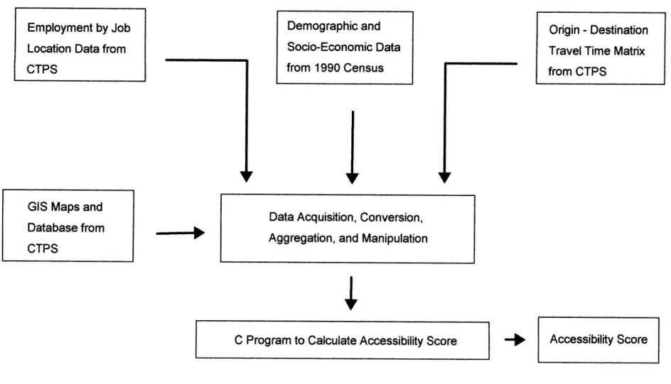
Procedure for Employment Accessibility Calculation
The procedure for employment accessibility calculation can be classified in the following 2 major steps: 1. Data collection, conversion, and manipulation, and 2.
Calculation of the employment accessibility. The procedure is discussed in details below. Figure 3.7 shows the flow chart for the procedure.
1. Data Collection, conversion, and manipulation
As indicated in section 2.1.2, data from many different sources were used in the computation of employment accessibility. After gathering data, the next step was to convert the data into a format that can be incorporated into the accessibility calculation. The conversion and manipulation include aggregation level
conversion, file format conversion, and redundant character elimination, etc.. 2 Employment Accessibility Computation
To calculate the employment accessibility, a C program was written to handle the task. The program took employment location data, labor force data, travel time by public transit, travel time by automobile, and automobile ownership data into the calculation. The program generated 2 sets of data, employment accessibility by automobile and employment accessibility by public transit. These 2 accessibility data were later incorporated into the regression analysis of housing price model described in section 2.2.4.
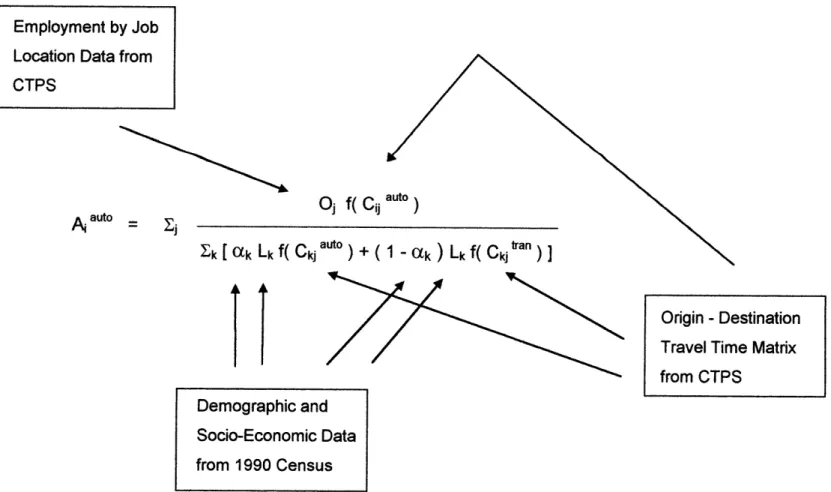
Figure 3.6
Data Sources of Accessibility Calculation
pAauto= Oj f(
Cj
auto)Ek [ ak Lk f( Ckj"") + ( 1 - aX ) Lk f( C tan
Employment by Job Location Data from
CTPS
Demographic and Socio-Economic Data from 1990 Census
Origin - Destination
Travel Time Matrix from CTPS
Figure 3.7
Procedures of Accessibility Calculation
C Program to Calculate Accessibility Score
Employment by Job Location Data from
CTPS
Demographic and Socio-Economic Data from 1990 Census
Origin - Destination Travel Time Matrix from CTPS
GIS Maps and
Database from
CTPS
Data Acquisition, Conversion, Aggregation, and Manipulation