Dynamic Diffracting Trees
by
Giovanni M. Della-Libera
S.B. Mathematics,
S.B. Computer Science,
Massachusetts Institute of Technology (1996)
Submitted to the Department of Electrical Engineering and Computer Science
in partial fulfillment of the requirements for the degree of
Master of Engineering in Electrical Engineering and Computer Science
at the
MASSACHUSETTS INSTITUTE OF TECHNOLOGY
July 1996
@ Massachusetts Institute of Technology 1996. All rights reserved.
A uthor ...
...
.
.
...
.. ...
Department of Electrical Engineering and Computer Science
Certified by... ...
SNir
Shavit
Assistant Professor of Computer Science and Engineering
Thesis Supervisor
Certified by
...
.. ...
...Nancy Lynch
Cecil H. Green Professor of Computer Science and Engineering
Thesis Supervisor
(1
,
nil
A
Accepted by ...
...
Chairman, Del
ric R. Morgenthaler
mn Graduate Theses
···
T
2 19
,
q7
Dynamic Diffracting Trees
by
Giovanni M. Della-Libera
Submitted to the Department of Electrical Engineering and Computer Science on July 19, 1996, in partial fulfillment of the
requirements for the degree of
Master of Engineering in Electrical Engineering and Computer Science
Abstract
A shared counter is a concurrent object which provides the fetch-and-increment operation on a distributed system. Recently, diffracting trees have been introduced as shared counters which work well under high load. They efficiently divide high loads into lower loads that can quickly access lock-based counters that share the overall counting. Their throughputs have surpassed all other shared counters when heavily loaded. However, diffracting trees of differing depths are optimal for only a short load range. The ideal algorithm would scale from the simple queue-lock based counter to a collection of counters with a mechanism (such as a diffracting tree) to
distribute the load.
In this thesis, we present the dynamic diffracting tree, an object similar to a diffracting tree, but which can expand and collapse to better handle current access patterns and the memory layout of the object's data structure, providing true scalability and locality. This tree then assumes each diffracting tree over its optimal range, from the trivial diffracting tree, a lock-based counters, to larger trees that have a collection of lock-lock-based counters. This reactive design pushes consensus to the leaves of the tree, making agreement easier to achieve. It does so by taking advantage of cache-coherence to keep agreement at the higher contention areas of the tree.
Empirical evidence, collected on the Alewife cache-coherent multiprocessor and a distributed shared-memory simulator, shows that the dynamic diffracting tree provides throughput within a constant factor of optimal diffracting trees at all load levels. It also shows to be an effective competitor with load balancing algorithms in produce/consumer applications.
We believe that dynamic diffracting trees will provide fast and truly scalable implemen-tations of many primitives on multiprocessor systems, including shared counters, k-exclusion barriers, pools, stacks, and priority queues.
Thesis Supervisor: Nir Shavit
Title: Assistant Professor of Computer Science and Engineering
Thesis Supervisor: Nancy Lynch
Acknowledgments
I have so few people to thank, and so much space to do it in. Oops! Strike that. Reverse! I would like to thank Nir Shavit for suggesting this wonderful project and guiding me throughout its inception and development. We went through many different designs and changes, and I never thought we would find one that was efficient and easy to explain. I also would like to thank Nancy Lynch for her continued pursuit of correctness, which led me to discover the immense benefits that come with actually thinking carefully about my algorithm and designing invariants that prove its correctness. I never was so appreciative of induction as I am now. I also thank Nir and Nancy for responding with care and support to the various emails I mailed off in times of stress.
I thank all the friends that supported me in this time-consuming process, but several stand out brightly. Roberto De Prisco and Mandana Vaziri, both officemates over the course of the year, for working with me on problem sets and putting up with my incessant chatter. Carl Hibshman, a biology major and English specialist corrected my entire thesis, a rather long and difficult task. He not only fixed my many pluralization errors, but spotted some typos in my lemma proofs that would not have been discovered if he hadn't been actually trying to understand all of the proofs. Steven Steiner came over in my most troubling hour of proving distinctness and helped me organize my invariants, giving me the impetus necessary to finish the proof. Pratip Banerji and Abiyu Diro listened to my rantings and ravings about the difficulties in my proofs, always calming me down. Matthew Eckstein put me up for this last month as I had already moved all my worldly possessions to Seattle. Finally, Jeff Marshall actually put up with me for the entire second term as we set attendance records at the Galleria Food Court, putting up with all of my mindless musings about my work and inviting me over to relax after a long day at the proof shop.
Finally, I have to thank my family for all of their support over the last 5 years. After being here for 5 years, I had almost forgotten that statistically speaking, I shouldn't be here. But I am, and my family all flocked up to Boston to celebrate in my graduation. The love they have outpoured for me has kept me sane and hopefully my plan to transplant all of them to Seattle will eventually unfold. A special thanks to my mother and grandmothers, the loving women who have watched out for me ever since I came on this earth.
I wanted to put a quote about counting in my thesis. Some battle scene perhaps where a young lieutenant said "If only we knew how many forces they had." Or, picture the familiar marbles in a jug contest. A scene in which the winner remarked "It was just a matter of ratios." However, none really come to mind, so instead I will resort to my high school yearbook quote.
"An Optimist is one who does math with a pen" - Source Unknown
This is cheesy, I admit. But, I wonder what the comparable quote is for counting things. "An Optimist is one who counts with a diffracting tree?" For some reason though, I think an Optimist would just guess.
Contents
1 Introduction 13
1.1 Background ... ... ... . 13
1.2 G oals . . . 15
1.3 Dynamic Diffracting Trees ... 16
2 DDT Design 19 2.1 Diffracting Trees ... .. ... ... . 19
2.1.1 Balancers ... .... ... . 19
2.1.2 Counters ... . ... ... . 22
2.2 Dynamic Diffracting Trees ... ... .. ... ... 22
2.2.1 Irregular Diffracting Trees ... ... 23
2.2.2 State and Versioning Information . . . 24
2.2.3 Folding and UnFolding ... ... ... 27
2.3 Bookkeeping .. ... ... 34
2.4 Cache Sizing . . . . ... 35
2.5 Folding and Unfolding Policy . . . ... 35
3 Experimental Results 37 3.1 Experimental Environments ... 37
3.2 Index Distribution Benchmark ... ... 38
3.2.1 Diffracting Trees and Queue Locks ... .... . 39
3.2.2 Alewife Results ... 40
3.2.3 DDT Results on Proteus ... 44
3.3 Large Contention Change Benchmark ... 49
3.3.1 Sudden Surge ... 49
3.3.2 Sudden Drop ... 50
3.4 Producer/Consumer Benchmarks ... 51
3.4.1 10-Queens ... 52
3.4.2 Sparse Producer/Consumer Actions ... .. 53
4 DDT Formal Model 55 4.1 User I/O Automaton ... ... ... 57
4.2 Balancer I/O Automaton ... 57
4.3 Tree Structure ... ... .. 58
4.3.1 Restrictions on Status ... 61
4.4 Main I/O Automaton ... 61
5 Automaton Verification 65 5.1 Distinctness . . . .. . . . ... . .. . . 65
5.1.1 M ulti-Sets ... ... ... ... ... 65
5.1.2 Outputs definition ... 66
5.1.3 Value Sets ... 66
5.1.4 Status Restrictions on Counters ... 69
5.1.5 Count Properties ... 70
5.1.6 Count Never Decreases ... 72
5.1.7 CounterLimit Count properties
5.1.8 Final Count Properties ... 75
5.1.9 Conclusion ... 77
5.2 Output Value Limit ... 78
5.2.1 M athematical Facts ... 78
5.2.2 Limits and Value Sets Revisited ... 79
5.2.3 ID, Status, and Balancer Properties ... 81
5.2.4 Active Processor Tracking ... 82
5.2.5 ID tracking ... 83
5.2.6 PathID tracking ... 84
5.2.7 Processor Travel Plans ... 87
5.2.8 Conservation of Energy ... 88 5.2.9 Conclusion ... 99 5.3 Safety Property ... .. ... .. 99 6 Implementation Verification 101 6.1 Request . . . .101 6.2 Increment Count ... 102 6.3 Return ... ... ... ... ... .. ... .. . ... ... ... .. . .. ... 102 6.4 BalancerRequest ... ... 102 6.5 BalancerReturn ... 103 6.6 Fold . . . .103 6.7 UnFold . . . .103 6.8 Liveness . . . .103
7.1 Continued W ork ... 106
7.1.1 More Performance Results ... 106
7.1.2 Completion of Implementation Proof . ... .. 106
7.1.3 W ait-Free Version ... 107 7.1.4 Timing Scheme ... ... 107 7.2 Future W ork ... 107 7.2.1 Message Passing ... ... 107 7.2.2 Elimination Trees ... ... 108 7.2.3 Scaling Policies ... ... 108
List of Figures
2-1 2-2 2-3 2-4 2-5 2-6 2-7 2-8 2-9 2-10 2-11 2-12 A Balancer at work . . . . ...Code for Balancing . .. . . . ...
A counting diffracting tree . . . .
An irregular diffracting tree's counting scheme . .
Definition of node structure . . . .
Key elements of a DDT node . . . .
Code for main traversal of DDT . . . .
Code for counting in DDT . . . .
Code for folding ...
Two cases of Folding, Parent node at Level 1 . . .
Two cases of Unfolding, Parent node at Level 1 . .
Code for unfolding ...
3-1 Diffracting Trees of depth 3 with Queue or Spin Locks at Counters on Proteus 3-2 Average Latency of Queue or Spin Lock Counters on Diffracting Tree of depth 3
on Proteus . . . .
3-3 Diffracting Trees, Queue-Lock Based Counter, and DDT on Alewife from 1-32 Processors . . . .
3-4 Throughputs of Optimal Composite vs. DDT on Alewife . . . .
3-5 Latencies of Optimal Composite vs. DDT on Alewife . ... 43
3-6 Diffracting Trees, Queue-Lock Based Counter, and DDT on Proteus from 1-32 Processors . . . 44
3-7 Throughputs of Optimal Composite on Proteus and normalized Alewife .... . 45
3-8 Throughputs of Diffracting Trees and Queue Lock on Proteus . ... 46
3-9 Latencies of Diffracting Trees and Queue Lock on Proteus . ... 46
3-10 Throughputs of Optimal Composite vs. DDT under high contention on Proteus . 47 3-11 Latencies of Optimal Composite vs. DDT under high contention on Proteus . . . 47
3-12 Throughputs of Optimal Composite vs. DDT under lower contention on Proteus 48 3-13 Latencies of Optimal Composite vs. DDT under lower contention on Proteus . . 48
3-14 Average latency of DDT over time in response to sudden surge . ... 50
3-15 Comparison of surges with dynamic and static prism sizing . ... 51
3-16 Average latency of DDT over time in response to sudden drop ... 52
3-17 10-Queens Performance and Code ... 53
3-18 Producer/Consumer Performance and Code ... .. 54
4-1 Interaction between Well-Formed Users, the Shared Memory System, and Balancers 56 4-2 Balancer I/O Automaton ... 58
4-3 Main I/O Automaton ... 62
List of Tables
5.1 Conservation of Energy definitions ... 91
Chapter 1
Introduction
Coordination problems on multiprocessor systems have received much attention recently. Shared counters in particular are an important area of study because the fetch-and-increment operation is a primitive that is being widely used in concurrent algorithm design. Since good hardware support is not readily available, there have been a variety of solutions presented for this problem in software.
1.1
Background
Simple solutions often involve protecting a critical section with either test-and-set locks with exponential backoff (spin-locks) by Agarwal, Anderson, and Graunke [2, 3, 10] or the queue-locks of Anderson or Mellor-Crummey and Scott [3, 15]. These algorithms are popular because they provide great latencies in low load situations, when requests are sparse and mostly sequential in nature. However, they can not hope to obtain good throughput under high loads due to the bottleneck inherent in mutual exclusion.
More sophisticated algorithms proposed have included the combining trees of Yew, Tzeng, and Lawrie [21] and Goodman, Vernon, and Woest [9], the counting networks of Aspnes, Her-lihy, and Shavit [4], and the diffracting trees of Shavit and Zemach [20, 18]. These methods are distributed and lower the contention on individual memory locations, allowing for better performance at high loads.
the requests that travel up the tree from the leaves. A single processor reaches the counter with several requests, which it can perform by incrementing the counter with the appropriate offset. This tree takes advantage of contention, so performs much better than a simple lock-based counter. The binary tree provides n processors with at best a time of O(log n) and a throughput of n/2 log n indices per time step. The pitfall with combining trees is that a single processor's
delay or failure in traversing the tree delays those that combined with it indefinitely.
A Bitonic counting network [4] is a data structure isomorphic to Batcher's Bitonic sorting network [5], with a "local counter" at the end of each output wire. At a junction in the network, the first processor that arrives exits on the top wire, the next on the bottom wire, and it continually oscillates. This is the first kind of tree to break away from a single lock-based
counter at its root, distributing the counting to several lock-based counters that count with fixed offsets. This allows requests to be independent, making it fault tolerant. These networks have width w < n and depth O(log2 w). At their best, the throughput is w and latency a high
O(log2 w). The biggest disadvantage with counting networks is their rigid network structure.
It is unclear how to change the structure of the tree.
The key advantage of counting networks are the k lock-based counters. If the load is too high for a lock-based counter to be effective, divide-and-conquer would encourage the load to be divided into pieces that can rapidly access a lock-based counter. By doing so, the k lock-based counters can efficiently move their lower loads through the shared counter, so the focus shifts to the mechanism for dividing the load. Diffracting trees [20] provide the most effective tool for distributing the load. The trivial Diffracting tree is just a simple lock-based counter. Once the load is high enough that division would benefit performance, diffracting trees of various depths can be used to effectively divide the load. They are constructed from simple one-input two-output computing elements called balancers that are connected to one another by wires to form a balanced binary tree. These balancers evenly divide their requests amongst their children. This tree of balancers can then quickly distribute requests to its output wires, which can be connected up to k lock-based counters for a high-performance distributed shared counter. Diffracting trees of various depths provide optimal performance throughout the load range, and the trivial diffracting tree, a queue-lock, provides the best performance under low load. However, a diffracting tree of a certain depth has unwanted costs for lower loads due to
The prior art seems to be firmly divided into two camps: the lock-based algorithms which work well in the low load cases and the distributed algorithms that do better under high load. The lock-based algorithms are championed by queue-locks and the distributed algorithms are currently led by Diffracting Trees. One set of experiments revealed that in a low load situation, the throughput over a fixed period of time for a queue-lock counter was 652 operations while the diffracting delivered 46 operations. With the same period of time but with a high load, the queue-lock counter went down to 595 operations, while the diffracting tree rose to 5010 operations. A factor of 10 difference separates each of these sets of numbers.
1.2
Goals
Diffracting trees, from the simple queue-lock based counters to large trees with a collection of counters, provide optimal performance at all load levels. Our goal is to make the diffracting tree structure dynamic, so it can react to the current load and assume the optimal size, guaranteeing the best possible performance.
B.H. Lim recently came up with a reactive scheme [11, 12] that switched between a test-test-and-set lock by Rudolph [17], a queue lock, and a combining tree. This performed well from the low to mid-load ranges, as the combining tree took over for the queue lock. His algorithm only applies to algorithms that have one centralized lock-based counter, which precludes diffracting trees, but gave valuable insights to reactive policy making.
We now focus on the two main insights necessary to create such an algorithm.
* Localize decision making
* Use cache-coherence to make global agreement inexpensive
Localized decision making spares processors from continually deciding on the overall struc-ture of the shared counter, which is what Lim's algorithm requires. A major drawback with global decision making is that processors can get delayed while they wait for a change to oc-cur. By making the changes in the shared counter local to only part of the counter, then the number of processors directly delayed drops significantly, and when other processors arrive in the changed part of the structure, the decision has been made and they can quickly adapt.
Cache-coherence makes localized decision making a reality. Keeping processors in agreement globally is usually an expensive requirement. If an algorithm adds global state which does not often change in high load situations, then this information can be cached, making constant reference to it an inexpensive proposition. If the load in an area of the tree is low, then changes can be made without high cost, which enables localized decision making.
1.3
Dynamic Diffracting Trees
Our algorithm, the Dynamic Diffracting Tree (or DDT), uses these two principles to make diffracting trees dynamic and reactive. A significant change in the load of the system will cause the DDT to expand or collapse into the optimal tree. These changes occur at the end of the tree, a local decision, but one that should be mirrored by the other ends of the tree in a genuine change of load. However, if the tree's memory layout is designed so that different ends of the trees exist in separate parts of memory, the tree may become irregularly formed to give optimal performance. State is added to the nodes of the tree to indicate what kind of node they are, and the caching of this state enables processors to pass through the tree without much delay.
We describe an implementation of the DDT concurrently with a thorough discussion of how the algorithm works. We discuss the scaling policies and the requirements that they must have, and describe the one that was implemented.
We implement the DDT on the MIT Alewife machine of Agarwal, Chaiken, Johnson, Krantz, Kubiatowicz, Kurihara, Lim, Maa, and Nussbaumet [1]. However, the largest Alewife machine only has 32 nodes, limiting the load range we could test with. We show that the Proteus Parallel Hardware Simulator of Brewer, Dellarocas, Colbrook and Weihl [6, 7], which we run up to 256 processes, simulates Alewife well, giving results that are comparable when normalized. We obtain results from various experiments, comparing the DDT to optimal diffracting trees of various depths, simple queue-locks, and implementing a job queue to compete with the load balancing scheme by Rudolph, Slivkin-Allalouf, and Upfal[16]. In the same experiment we ran earlier, the DDT under low load provides 243 operations and under high load provides 3932 operations. The results show that the DDT performs within a constant factor of optimal diffracting trees at all load levels, and future work shows good promise in lowering this factor. A particularly interesting result on the MIT Alewife machine shows a range where the DDT
outperforms all regular Diffracting Trees due to its ability to assume an irregularly-shaped tree structure, taking advantage of locality. We also show that the DDT performs effectively in Producer/Consumer applications.
We define safety and liveness properties that any shared counter should satisfy. We present a specification of the DDT using the I/O Automata of Lynch and Tuttle [13] and formally prove that it satisfies these properties. We sketch an argument which shows that the implementation presented meets the specification.
In summary, we believe that the DDT and its underlying concepts will prove to be an effec-tive paradigm for the design of future data structures and algorithms for multi-scale computing.
This paper is organized as follows: Chapter 2 explains the design of the DDT, presenting the asynchronous shared-memory implementation, and discusses different scaling policies, Chapter 3 discusses the performance results on Alewife and Proteus, Chapter 4 gives the formal description of the DDT, Chapter 5 gives the proof of the specification, Chapter 6 presents the argument that the implementation meets the specification, and Chapter 7 concludes this paper and lists areas of further research.
Chapter 2
DDT Design
We begin by reviewing the basics of diffracting trees and describe in detail the changes necessary to make them dynamic. This includes an implementation of the DDT on an asynchronous, cache-coherent, distributed shared-memory system. Finally, the scaling policy issue is discussed.
2.1
Diffracting Trees
A Diffracting tree [20] consists of balancers that are connected to one another by wires in the form of a balanced binary tree, and local counters attached to the final output wires of the tree. A balancer's job is to continually split the number of requests on its input wires onto its two output wires. A local counter counts with an increment based on its depth into the tree, and although its implementation is not restricted, it is assumed that it is a lock-based counter.
2.1.1 Balancers
First, we give the requirements that a balancer must satisfy. We denote by x the number of input requests, or tokens, ever received on the balancer's input wire, and by yi, i E {0, 1} the number of tokens ever output on its ith output wire. Given any finite number of input tokens
x, it is guaranteed that within a finite amount of time, the balancer will reach a quiescent state,
that is, one in which the sets of input and output tokens are the same. In any quiescent state,
yo = [x/2] and y, =
Lx/2].
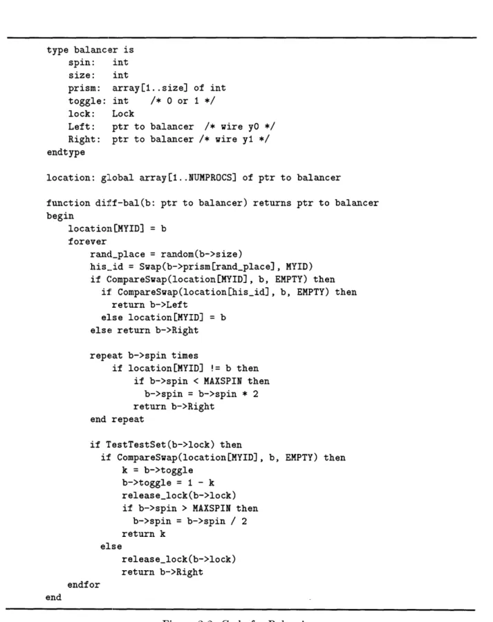
Figure 2-1 shows how a balancer could split up 9 distinct process requests (A-I), where the requests without spaces between them happen at the same time.I H GFE DCBA
l
CABEFI
V1 CDGH
Figure 2-1: A Balancer at work
A simple implementation of a balancer would be a memory location with a lock that toggles between the values 0 and 1. A token entering the balancer obtains the lock, gets the value, stores the inverse value, and exits on the wire indexed by the value obtained, unlocking the bit. This clearly satisfies the properties above, but the lock reduces this problem to the same as that of a lock-based counter, and does nothing to reduce the bottleneck.
Shavit and Zemach present a much better implementation of a balancer [20], which exploits large numbers of requests to pair off processors onto the two output wires and avoid contention. When a processor enters a balancer, it enters that balancer's ID in its position in a global location array, selects a random location in that balancer's prism, and swaps the processor's own ID into that location. It attempts to pair off with the processor ID that it receives from the swap. If it fails, it then spins for a certain amount of time waiting for a processor to choose it. If all else fails, it attempts to access the test-and-test-and-set [17] lock described above. If it fails, then it starts all over, trying to reenter the prism [18]. This algorithm is really just an optimization since two processors flipping the bit would leave it unchanged. Figure 2-2 shows the code for the balancing code. This algorithm has been shown to satisfy the properties above [20].
The most important parameters for a diffracting tree are the sizes of the prisms and the spin constants mentioned above. Shavit and Zemach's steady-state analysis [18] found that a tree that would serve P processes should have a depth d and a number of prism locations L such that 1 = 0(1), L < d, and L = cd2d, where c is a machine-dependent constant. Given
the approximate range of load that a diffracting tree would get, a developer can then choose d and subsequently decides upon L. A reactive backoff scheme was also implemented in [18] to provide the best spin constant.
type balancer is spin: int
size: int
prism: array[1..size] of int
toggle: int /* 0 or 1 */ lock: Lock
Left: ptr to balancer /* wire yO */ Right: ptr to balancer /* wire yl */
endtype
location: global array[l..NUMPROCS] of ptr to balancer
function diff-bal(b: ptr to balancer) returns ptr to balancer begin
location[MYID] = b
forever
randplace = random(b->size)
his--id = Swap(b->prism[randplace], MYID) if CompareSwap(location[MYID], b, EMPTY) then
if CompareSwap(location[hisid], b, EMPTY) then return b->Left
else location[MYID] = b
else return b->Right repeat b->spin times
if location[MYID] != b then if b->spin < MAXSPIN then
b->spin = b->spin * 2
return b->Right end repeat
if TestTestSet(b->lock) then
if CompareSwap(location[MYID], b, EMPTY) then
k = b->toggle b->toggle = I - k
release_lock(b->lock) if b->spin > MAXSPIN then
b->spin = b->spin / 2 return k else release_lock(b->lock) return b->Right endfor end
2.1.2
Counters
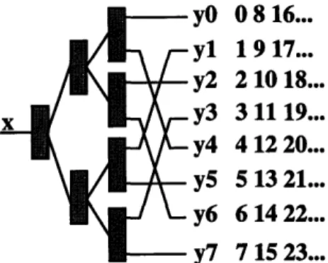
The counters at the end of the tree have an increment equal to their depth into the tree. Their initial values are based on their position in the tree. The "Leftmost" counter, or counter at which a single entrant to the tree would arrive, has initial value 0. The counter with initial value 1 would be the "Leftmost" counter of the subtree rooted by the main root's Right child. It is clear how the ordering then proceeds. Figure 2-3 shows a diffracting tree of size 8 with its output wires ordered for counting.
08 16...
1 9 17...
210 18...
31119...
4 12 20...5 13 21...
6 14 22...
7 15 23...
Figure 2-3: A counting diffracting tree
The algorithm for traversing the tree is clear. A token starts at a root node, and balances until it reaches a leaf counter, at which point it interacts with the counter, obtains a value, and exits.
2.2
Dynamic Diffracting Trees
We now start to move to a less rigid structure. Our goal is to allow Dynamic Diffracting Trees to control the following three parameters:
* Depth of Tree
* Prism Sizes
* Spin
By doing so, we gain full control of the parameters on page 2.1.1 that can be set to craft the optimal diffracting tree for a given load. We will employ localized decision making to allow
the tree to change height. As the number of processors P and subsequently the load changes, the tree would optimally expand or collapse to result in the best d and L possible, with the spin constant still determined by the reactive backoff scheme designed in [18].
We now individually discuss each loosening or addition to the original diffracting tree.
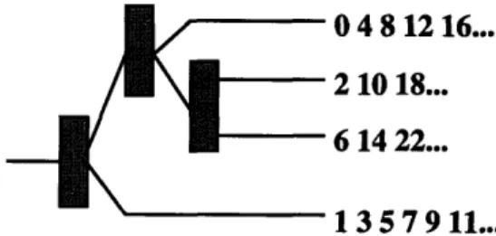
2.2.1 Irregular Diffracting Trees
In this kind of tree, we relax the restriction that the tree must be balanced. We only require that balancers have two children and counters are only at leaves. It should be clear that this restriction is not necessary for the algorithm to work correctly, and was instead placed under the assumption that a balanced tree gives the best performance. Abstractly, each balancer and its subtree represents an implementation of a counter, so it could be replaced by a lock-based counter and still function correctly. Figure 2-4 shows how one would set the counter's increment and initial values to make it work correctly.
04 8 12
16...
2 10 18...
6 14 22...
1 3 D / 11...
Figure 2-4: An irregular diffracting tree's counting scheme
The reason we must consider this is because it would be very expensive to change an entire diffracting tree to a different size. However, processors can work on different leaves in the tree, expanding or shrinking locally, causing the tree to be irregular at times. It is expected that the rate-making policy at one leaf would ask for the same kind of change as another leaf, due to the average contention levels that the balancers distribute over the entire tree, but if locality dictated that certain ends of the tree were slower than other ends of the tree because of the memory layout of the data structure, then it would be optimal to make the tree irregular to maximize performance on that given memory layout.
2.2.2
State and Versioning Information
Now, once we let the tree size change, we could potentially get trapped into some alloca-tion/deallocation memory issues. We could run out of memory, allocation could take a very long time and bottleneck the processors, or a pointer to a deallocated node could remain around long enough to cause a problem if it was reallocated. Also, since we allow the trees to shrink and grow, it is no longer possible for every processor to initially memorize the structure of the tree, as it could in the diffracting or irregular diffracting tree. So, upon visiting a node of the tree, a processor would need to determine if that node was a counter or balancer.
We solve all of the above problems in the following way. We first add a state variable. This state variable initially only takes three variables, Counter, Balancer, or Off. The first two are clear in the context of merging the types of data structures together. A processor that visits a Balancer node balances, and one that visits a Counter node counts. However, if a processor visits an Off node, then it would know that the tree somehow changed beneath it, so it would trace up the node's ancestral path til it found a node it could successfully visit. We now solve the memory problems by creating a large, balanced tree then creating an initial configuration of balancers and counters from the root and leaving the rest of the tree Off. The designer can decide whether a real leaf of this tree can have an allocation call if it wishes to expand or if there is a static limit to the tree. Finally, we add a CounterLimit state for the case where the tree shrinks, which will be explained soon.
This state variable could potentially be an expensive item to check. If the state variable in the root of the tree continually changed, all processors accessing it would be consistently delayed, bringing performance down. However, a sensible scaling policy would prevent the root node to change under high loads. In doing so, processors can utilize cache-coherence to keep accesses to the top level state variables relatively inexpensive. This brings into mind the second main property of the introduction, keeping global agreement inexpensive.
This solution provides distinctness and does not attempt to keep the different parts of the tree in balance. To provide a good balance, a versioning scheme must also be added. More precisely, the goal is to prevent a number from being handed out beyond the current number of requests, to keep the counter in line with more traditional lock-based counters. To better understand how this could be violated with the current design, consider this scenario: The tree
consists of a simple balancer at the root and two child counters. Clearly, one counter hands out the even numbers and one the odd numbers. Assume that the first number to be handed out is 0, and there are 10 requests made. 5 requests go along each of the two wires. After the
10 requests have been sent out, the tree decides to shrink, becoming a counter at the root and making the two children Off. Assume that the 5 requests along the even wire arrive, see the Off state, and return to the parent, obtaining the first 5 values, 0,1,2,3, and 4. Now, the tree decides to unfold again, and it initializes the two counters to next hand out 5 and 6. Now, the other 5 requests arrive at the odd counter. They receive 5, 7, 9, 11, and 13. Notice the imbalance amongst the 10 numbers handed out.
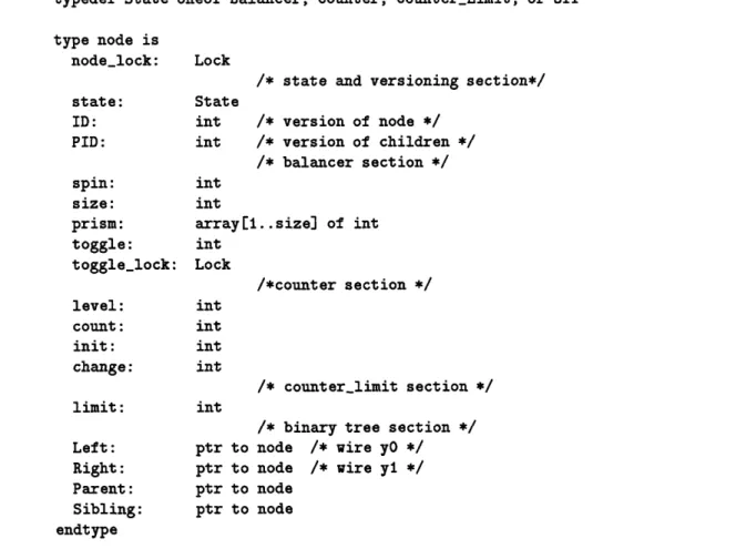
The key change needed to solve this is that once a balancer becomes a counter, all requests that have passed through that balancer and have not been satisfied have become delinquent. These delinquent processors need to come back to the node and access it again. The way to do this is to install a versioning scheme. When a balancer becomes a counter, the two children need to increase their version numbers, so that if a processor arrives at a node with a distinct version number' from that which its parent foretold, it would return to the parent and revisit, to get updated. Each processor caches the versioning numbers throughout its traversal of the tree, and if at any point it finds a differing version number, it traverses back up the tree until it finds agreeing version numbers, which in the worst case is the Root node whose version never changes. This versioning scheme can be folded into the state variable in an implementation, to reduce size and complexity, since versioning really is additional state. But, for simplicity, it is kept separate here. The definition of the new node structure is given in Figure 2-5.
'Technically, these version numbers are unbounded integers, but they are bounded by the values of the counters, so any implementation which handled the overflow of the counters could handle this as well.
typedef State oneof Balancer, Counter, CounterLimit, or Off type node is node_lock: state: ID: PID: spin: size: prism: toggle: togglelock: level: count:
init:
change: limit: Left: Right: Parent: Sibling: endtype Lock/* state and versioning section*/ State
int /* version of node */ int /* version of children */
/* balancer section */
int
int
array[1..size] of intint
Lock /*counter section */int
int
int
int
/* counter-limit section */int
ptr ptr ptr ptr/* binary tree section */ node /* wire yO */
node /* wire yl */
node node
Figure 2-5: Definition of node structure
7
K
Fo-
lou
CM- Limit State CountFigure 2-7 contains the code for the main traversal of a processor through a dynamic diffract-ing tree. The Bookkeepdiffract-ing work is explained later in this chapter. Figure 2-8 contains the new code for accessing a Counter or CounterLimit (which will be explained in the next section).
root: global ptr to node /* main root of Bookkeeping: global array [I..NUMPROCS] of
function fetch.incr() returns int
answer: int
IDRecord: array
[enumeration
of nodes]n: ptr to node begin IDRecord[root] = 0 n = root answer =: INVALID forever
if (n->ID != IDRecord[n]) then n = n->Parent continue tree */ pair
of int
switch n->state case Balancer: Bookkeeping MYID] = <n>if ((n->state != Balancer)
II
(n->ID != IDRecordEn]))n = n->Parent continue
IDRecord[n->Left] = n->PID IDRecordEn->Right] = n->PID
if n->state == Balancer then
n = diff-bal(n)
case Off:
n = n->Parent;
case Counter or Counter_Limit: answer = incrementcounter(n); if valid(answer) then return answer else n = n->Parent endswitch endfor end
Figure 2-7: Code for main traversal of DDT
2.2.3 Folding and UnFolding
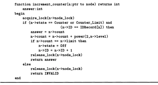
We now describe how the changes in the tree work. The operation occurs locally at the bottom of the tree, folding two sibling counters into their parent balancer, becoming a new counter, or
function increment_counter(n:ptr to node) returns int answer: int
begin
acquirelock(n->nodelock)
if (n->state == Counter or CounterLimit) and
(n->ID == IDRecord[n]) then
answer = n->count
n->count = n->count + power(2,n->level) if n->count == n->limit then
n->state = Off n->ID = n->ID + 1 release_lock(n->nodelock) return answer else release_lock(n->nodelock) return INVALID end
Figure 2-8: Code for counting in DDT
unfolding a counter into a balancer with two counter children. The algorithms we present here
involve possessing 3 locks at one time, but this should be adaptable to having 1 lock at a time in the eventual goal of making this algorithm wait-free. We avoid this complication, however, because it adds extra state to the system and obfuscates the actions which occur. We describe
each change below:
Folding
Figure 2-9 contains the code for folding. A processor, upon deciding that a balancer and its children counters need to be folded will attempt to obtain all 3 locks. If it is successful, then it tests whether the 3 nodes are a balancer with two child counters.
function attempt_fold(n:ptr to node) returns boolean nLeft, nRight, nMax, nMin: ptr to node
valLimit: int begin nLeft = n->Left nRight = n->Right acquire lock(nLeft->togglelock) acquirelock(nRight->togglelock) acquire_lock(n->togglelock)
if (n->state == Balancer) and
(nLeft->state == Counter) and (nRight->state == Counter) and
((nLeft->count != nLeft->change) or (nRight->count != nRight->change)) then
n->state = Counter n->PID = n->PID + 1
valLimit = MAX(nLeft->count,nRight->count) - power(2,n->Level)
n->count = valLimit n->change = n->count
Assign nMin, nMax to be nLeft, nRight, such that nMin->count < nMax->count
nMax->state = Off
nMax->ID = nMax->ID + 1
if nMin->count < valLimit then
nMin->state = Counter_Limit nMin->limit = valLimit else nMin->state = Off nMin->ID = nMin->ID + 1 releaselock(nRight->node_lock) releaselock(nLeft->nodelock) release lock(n->node-lock) return TRUE else release lock(nRight->plock) releasejlock(nLeft->plock) releaselock (n->plock) return FALSE end
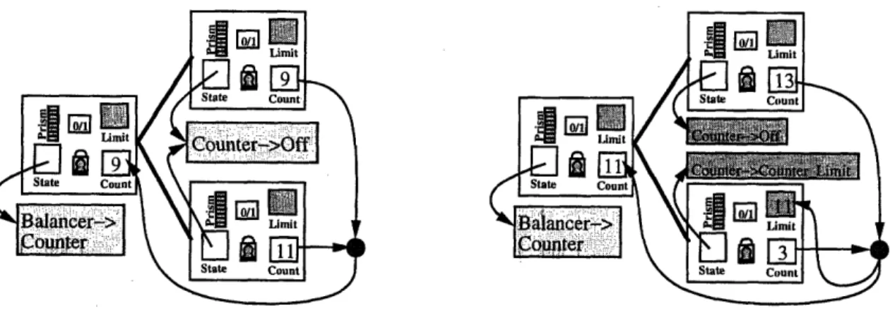
Once the locks are obtained and the states are checked, the two child counters' values are compared. Now, the values these two counters hand out are intertwined. They are obviously values that their parent would have handed out as a counter, and they share between them all the values their parent would have handed out, alternating between them. Imagine enumerating a list of numbers that their parent would hand out if it was a counter. Then, one of the child counters hands out the values which appear in the odd positions of the list, and the other hands out the even-indexed values. The ideal situation in folding is that the two counters' values are adjacent on the list. Now, the value contained in the counter's register is the next value to be handed out. If they are adjacent, the parent counter can be set to next hand out the lower of the two numbers, the states are changed (the children are turned Off), and the parent is ready to start counting. This is demonstrated by the first picture in Figure 2-10.
Figure 2-10: Two cases of Folding, Parent node at Level 1
Now, there are cases where the two counters' values are not adjacent on this list. This is the case where some reasoning is required. We take the maximum of the two values, find its position on the list, and move down one notch. This next-lower value on the list is the
limit value, and it is the value assigned to the parent counter. Now, this limit value would
normally be handed out by the smaller counter, since adjacent elements on the parent's list are handed out by the different counters. We make the smaller counter a CounterLimit, which acts just like a Counter, except it has a limit assigned to it of the limit value. If the smaller counter's value reaches the limit value, it turns Off and hands out no more values. The larger counter is immediately turned Off. It is clear that this scheme avoids any over-counting, and a demonstration is presented in the second picture in Figure 2-10.
up all of its available numbers. The parent becomes a Counter, so it does not balance any more processors towards it, and unfolding cannot occur if one of a Counter's children is a Counter_Limit. This is formally proven in the verification section, but informally, the reasoning is as follows: Either these sibling counters have been running from the beginning, or they were unfolded at some point. During unfolding, the values placed in sibling counters are initially adjacent on their parent's list. This is also true upon initialization of the tree. The balancing that occurs has the property that the requests are essentially evenly split amongst the two children. The key insight then is that if one counter's value is more than one higher on the list than the other counter, then it has satisfied more requests. But, due to the balancing process, the other counter should receive the same number of requests, which would let it catch up and fill up all of its values. (It could receive a maximum of one less, but that would imply that it was second on the balancing, which would imply that it started initially larger than the other counter, recovering the one to maintain the balance and allow the adjacency to eventually occur.)
This key insight is what allows this algorithm to work quickly. A scheme could be imple-mented that allowed for storing the values that weren't handed out in a queue, but this would add another level of complexity and decrease performance.
Unfolding
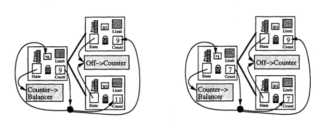
Unfolding is a bit easier to understand, but has its own challenges. Figure 2-12 contains the code. The same 3 locks are set, the states are checked (we can only unfold a Counter with two Off children.), and then we do the obvious settings. The current counter value can be set to one of the child counters. The next value is then set to the other child counter. Now, the problem here is that we want the balancing to occur so that the extra request always goes to the smaller child counter value. We do this by setting the balancer's toggle bit in the direction of the child with the smaller value. The two different cases are shown in Figure 2-11.
An alternative to the above algorithm would be to keep consistent the role of the Left or first child as the primary child in balancing. Then, the smaller value would always go here. Since the toggle bit would then always be reset to 0, it is just a technical difference. The advantage to the chosen scheme is that it allows each node to have a consistent set of values from which it hands out, simplifying the verification process. In this alternate scheme, each unfolding could
Figure 2-11: Two cases of Unfolding, Parent node at Level 1
assign to a child node a distinct class of values to hand out that it didn't before.
The biggest problem with unfolding is primarily an implementation issue. Consider when these actions would occur. Folding would occur because of below-average contention in that area of the tree. There isn't much delay when the locks are set, since there just aren't that many processors around. On the other hand, unfolding can be a costly process, since it occurs because of high contention. The code presented here releases the parent lock as soon as it's state is set, so that the processors that are waiting to access the counter can sooner find out that it is now a balancer and balance. Some optimizations performed here include having the lock.releaser go through and tell all of the processors waiting in the queue that the state has changed, so they can diffract, which gives the balancer a good start with high contention. A future optimization could lie in implementing a tree lock instead of a queue lock so this release could occur even faster.
A specification of this algorithm is proved correct in Chapter 5, and an argument is sketched in Chapter 6 about the correctness of this implementation.
function attempt_unfold(n:ptr to node) returns boolean nLeft, nRight: ptr to node
val, ID, i: int begin
nLeft = n->Left
nRight = n->Right
ID = n->ID
for i from 1 to NUMPROCS
if (Bookkeeping[il = n) return FALSE; acquirelock(nLeft->togglelock)
acquire_lock(nRight->togglelock) acquirelock(n->togglelock)
if (n->state == Counter) and (n->count != n->change) and
(nLeft->state == Off) and (nRight->state == Off) and
(n->ID == ID) then
n->state = Balancer
n->PID = n->PID + 1
val = n->count
if ((val - n->init) / power(2,n->level)) mod 2 == 1
n->toggle = 1 else n->toggle = 0 release_lock(n->toggle lock) nLeft->state = Counter nRight->state = Counter nLeft->ID = nLeft->ID + 1 nRight->ID = nRight->ID + 1
if ((val - n->init) / power(2,n->level)) mod 2 == 1
nRight->count = val
nLeft->count = val + power(2,n->level)
else
nLeft->count = val
nRight->count = val + power(2,n->level) nLeft->change = nLeft->count nRight->change = nRight->count releaselock(nRight->toggle-lock) release lock(nLeft->togglelock) return TRUE else release_lock(nRight->toggle_lock) release-lock(nLeft->togglelock) release-lock(n->togglelock) return FALSE end
2.3
Bookkeeping
The missing item from the unfolding section was Bookkeeping. We now explain its necessity. A Balancer, upon folding into a Counter, now must force all of the delinquent processors that balanced through it to now return. Versioning causes this to happen. However, imagine that the node now wishes to unfold again. If it becomes a Balancer, then new processors will balance through it and have correct forecasts for the new child Counters. However, imagine a processor that visited the node in its first incarnation as a Balancer. It received the forecast for its children, then also Counters, and began to balance. While it was attempting to diffract or access the toggle bit, all of these changes were to occur, and the node now went into its second incarnation as a Balancer. If this old processor were to diffract against a new processor, then it would upset the balance of the system, since it would arrive at one child Counter, find an incorrect version number, and return to the parent, while its partner from diffraction would arrive at the other child Counter and correctly access it. Now, imagine this happened potentially many times, and each time the old processor went towards the same Counter. When it came time to fold again, there would be no processors left that could bring the troubled Counter back into balance with its sibling.
The solution to this is simple, and the code is given in the main traversal (Figure 2-7) and unfolding code (Figure 2-12). We create a global bookkeeping array, one in which every processor has an entry. A processor, upon visiting a Balancer, registers in its entry of the array the balancer it is visiting. It then rechecks to make sure that the node is still a Balancer with the forecasted ID and enters the balancing section of the code. If the information on the second check was inconsistent with the processor's remembrance, it will go up the tree until it gets back on track. Now, the final piece is a restriction on unfolding. In order for a processor to unfold a Counter, it must traverse the bookkeeping array and make sure no processor is registered as visiting this node as a Balancer. If this traversal is successful, it then unfolds the node if the ID was the same as before the traversal. This is correct for the following reason. A processor sees that the node is a Balancer and puts itself into its array location. An unfolding processor saw that the node was a Counter and that the first processor's bookkeeping entry did not have this node registered. The ordering of these events on a machine that guarantees atomicity per memory location, (as our Alewife machine does guarantee [8], implies that either the first processor will see the update upon its recheck, or the unfolding processor will learn that it was
out of date and will not unfold.
2.4
Cache Sizing
The size of the cache is an interesting study on its own. The steady-state analysis [18] predicts that there should be cd2d prism locations in the tree, where c is a constant and d is the depth. Now, in this tree, we have changing depths. The solution is for each processor to keep a notion of the tree's current depth. A skeletal cache of the state is enough for a processor to average the depths of the various paths into the tree and come up with an average depth. Given the best experimental constant c and a large enough prism to handle the largest allowed tree, processors can then simply pick a value randomly within their expected prism size. It is expected that in practice eventually processors will approach the same average depth computation, providing the most efficient balancing regardless of the size of the tree.
2.5
Folding and Unfolding Policy
There are three main qualifications that a good scaling policy should meet.
* A policy should react quickly to large changes in the load.
* A policy should keep the overhead that it causes low and factor it into its decision making process
* A policy should keep the number of false positives low and limit many consecutive oscil-lations
Keeping this in mind, most of our policy exploration was focused on studying the contention at a counter lock. We felt that this was a good estimate for the overall load of the tree. If the lock was always empty when a processor arrived at the counter, then that counter should be folded into its parent. If the lock was always overloaded, then the counter should be unfolded. We found that observing the time it took to access the counter was a good measure. Queue locks have the nice property that the times measured are stable under consistent contention levels, unlike the oscill.ating times a spin lock would provide.
We then designed our policy around setting thresholds for these times. Passing below a folding threshold or taking longer than the unfolding threshold was a good indication that the local area should change. However, the data structure should not change based on the opinion of one processor. Our final policy is a variant of B.H. Lim's policy in his reactive data structure [11]. It uses a string of consecutive times to allow a change to occur. The minimum number of consecutive times was a constant that was decided upon by experimentation.
This met all three qualifications. A large change in the load will move the time consistently below or above these thresholds and allow for a change. The overhead is low since only one test is needed to see if the time is within the thresholds, stopping any current streaks and allowing the processor to continue. Finally, by requiring consecutive times, a nice hysteresis affect occurs, because it could not immediately change back in the other direction.
Future possibilities include on-line competitive schemes [14] or policies that measure the balancer performance. Since the balancers are tuned by the dynamic prism sizing, a study of the toggling behavior and diffracting rates could reveal a pattern which indicated when it should fold and when its children should unfold.
Chapter 3
Experimental Results
We evaluated a Dynamic Diffracting Tree by implementing it on both a multiprocessor machine and a simulator and running several experiments. The MIT Alewife machine developed by Agarwal et. al. [1] was the target machine for this implementation. However, the largest machine only has 32: nodes. We then ran the same experiments on the Proteus' simulator, developed by Brewer et. al. [7], where we were able to extend our results to 256 processes, and did a correlation to show that the results were comparable. The experiments we performed include index-distribution, sudden spikes and drops in load levels, and producer/consumer runs, all of which demonstrate the advantages of the DDT in a variety of applications.
3.1
Experimental Environments
The MIT Alewife machine consists of a multiprocessor with cache-coherent distributed shared memory. Each node consists of a Sparcle processor, an FPU, 64KB of cache memory, a 4MB portion of globally-addressable memory, the Caltech MRC network router, and the Alewife Communications and Memory Management Unit (CMMU). The CMMU implements a cache-coherent globally-shared address space with the LimitLESS cache-coherence protocol [8]. The LimitLESS cache-coherence protocol maintains a small number of directory pointers in hard-ware, and handles the rest in software. The Alewife machine guarantees sequential consistency on its cache-coherent memory locations, which means that any processor's memory transactions
are ordered consistent with their code base, and memory transactions on a memory location are processed as if they came from a FIFO queue. The Alewife LimitLESS cache coherency policy specifically upon receipt of a write request will require all processors to flush their cached copies of that variable and respond with an acknowledgment before granting the write request.
The primitive that Alewife provides as a read-modify-write operation is full/empty bits. Every memory location has a full/empty bit associated with it. This allows for mutual exclusion, since operations are provided which allow a processor to atomically set the bit full if empty and vice-versa. Given this, we deal more abstractly in our remaining discussion about mutual exclusion, taking for granted the availability of queue or spin locks.
Proteus multiplexes parallel threads on a single CPU to simulate the Alewife environment. Each thread has its own complete virtual environment, and Proteus records how much time each thread spends in its various components. In order to improve performance, Proteus does not completely simulate the hardware. Instead, local operations are run uninterrupted on the simulating machine, and this is timed in addition to the globally visible operations to derive the correct local time. This limits its ability to accurately simulate the cache-coherence policy. Proteus does not allow a thread to see global events outside of its local time environment.
3.2
Index Distribution Benchmark
Index-distribution is the simple algorithm of making a request and waiting some time before
the request is repeated. In this case, the amount of time between requests is randomly chosen between 0 and work, a constant that determines the amount of contention present. work = 0 represents the familiar counting benchmark, providing the highest possible contention for the number of processors given. A higher value, usually work = 1000 is chosen to give a lower-contention environment. This is a good benchmark to study because it is often used in load-balancing, when the tasks that the processors perform take a varying amount of time, but usually within some predictable level of work. We ran this benchmark for a fixed amount of time on the Alewife machine (10' cycles), varying the number of processors2 and the value of work. We also ran this benchmark on the Proteus simulator (105 cycles), and correlated the results. Since there are usually startup costs, the algorithms are run for some fixed time before
the timing begins. This brings into question the fact that the DDT will grow and shrink if the load does not meet well with its initial conditions. Since a separate experiment is conducted to test the changes of the DDT, a substantial startup period will be allowed before timing begins to allow the DDT to best match the input load.
The data collected were the average latency and throughput. The average latency is the average amount of time between the call to get.next_index() and its return. The throughput is the total number of get.next_index() operations that returned in the time allowed. These are clearly related numbers that can be approximately calculated from each other.
In this benchmark, the algorithms that were run were the Dynamic Diffracting Tree, Diffracting Trees of widths 2, 4, and 8 (and on Proteus, 16 and 32), and a queue-lock based counter. This queue-lock consists of a linked list of processors pointing towards their successors, waiting for their predecessors to wake them up once they are done with the lock. There is a tail pointer which directs new processors to the end of the queue. This code was implemented using atomic register-to-memory-swap and compare-and-swap operations.
3.2.1 Diffracting Trees and Queue Locks
We experimented with two variants of the Diffracting Tree algorithm and with several different prism sizes, and changed the diffracting tree algorithm to use queue-locks instead of spin-locks, which made their performance more robust. For each depth of the diffracting tree, we found the optimal prism size.
We tested both the original Diffracting Tree algorithm [20] and the alternate Diffracting Tree algorithm [18]. The alternate algorithm performed better at all depth and prism sizes. The main difference between these two algorithms occurs after the test-and-test-and-set operation on the toggle bit fails. In the original algorithm, a processor then waited longer to see if it got diffracted. In the alternate algorithm, a processor attempted to enter the prism again. This is better because a processor is more likely to diffract when it re-enters the prism then when it waits around.
The other major update of the original implementations is the use of queue-locks on the counters as opposed to spin-locks. Originally, a test-and-test-and-set loop repeated until it could acquire the lock and increment the counter. This caused the diffracting tree's throughput to
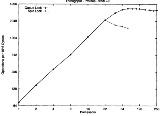
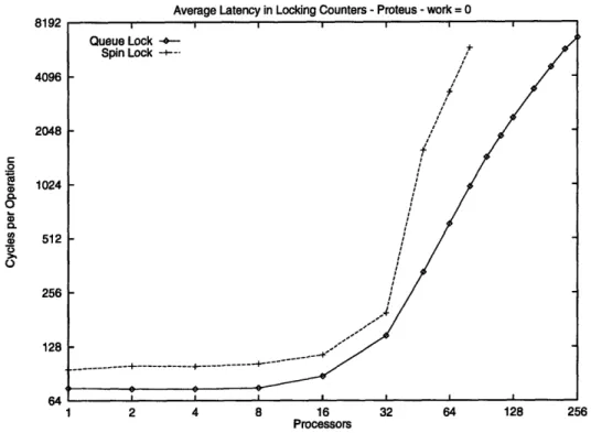
degrade after its peak due to contention. With the addition of a queue-lock, throughput remains steady as higher contention on the lock simply increases the waiting time for the queue. This makes the algorithm more robust, considerably extending the lifetime of a diffracting tree. Figure 3-1, shows a comparison of throughputs of optimal depth 3 diffracting trees with queue-and spin-locks, queue-and Figure 3-2 shows the average waiting time for the two counters.
4096
2048
1024
512
256
Throughput - Proteus -work = 0
2 4 8 16 32 64 128 256
Processors
Figure 3-1: Diffracting Trees of depth 3 with Queue or Spin Locks at Counters on Proteus
The Steady-State analysis [18] determined that there should be cd2d prism locations in the tree, with c2d locations on each level of the tree, where c is a constant. We experimented by comparing trees at each level and found that c = 1/2 was the best factor overall.
3.2.2 Alewife Results
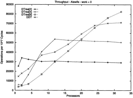
We have the first published performance results for Diffracting Trees on the Alewife machine. We implemented the Dynamic Diffracting Tree directly from the description given in Chapter 2. We configured the dynamic prism sizing to use the constant c found above. We set the number of consecutive timings before a change to be 80, a good experimental number that limited the number of oscillations. Our experiments also determined that the best fold and unfold threshold times were 150 and 800 cycles. Figure 3-3 shows throughputs for a queue-lock based counter,
Average Latency in Locking Counters - Proteus - work = 0 8192 4096 2048 a 1024 0 W 512 256 128 R4 1 2 4 8 16 32 64 128 256 Processors
Figure 3-2: Average Latency of Queue or Spin Lock Counters on Diffracting Tree of depth 3 on Proteus
diffracting trees of depth 1, 2, and 3, and the DDT. The most interesting result is that the DDT surpasses all of the diffracting trees shown for a brief range. This is due to its ability to expand only where needed, supplying irregularly sized trees which perform better in this range.
Since the Dynamic Diffracting Tree should represent optimal diffracting trees at each of their optimal points, we have constructed a composite graph of the diffracting tree and queue-lock counter through-puts, with the highest throughput from any diffracting tree or queue-queue-lock counter at a given load level chosen for the graph. We show the optimal composite vs. the DDT for the Alewife in Figures 3-4 and 3-5 under high contention. The throughput and latency appear to stay within a factor throughout its performance. The average factor between the throughput of the DDT and the optimal composite is 1.27.
90000 80000 70000 60000 50000 40000 30000 20000 10000 0 10 15 20 25 30 Processors
Figure 3-3: Diffracting Trees, Queue-Lock Based Counter, and Processors 131072 65536 32768 16384 092 DDT on Alewife from 1-32
Throughput - Alewife - work = 0
! I I Optimal Composite ---DDT - --->DTree[8] ue ->DTree[4(1 -QueueLock - ,,,-- .--- "* Processors
Figure 3-4: Throughputs of Optimal Composite vs. DDT on Alewife
Throughput - Alewife - work = 0 DTree[2] ---DTree[4] -+--- .-DTree[8] ---DDT . o-... . ... ... x 4 --- -Ole I s S ' ---- // o o-· oiJr
Average Latency - Alewife - work = 0
1 2 4 8 16
Processors
Figure 3-5: Latencies of Optimal Composite vs. DDT on Alewife
32 8192 4096 2048 0 CL 0. o 1024 (. a) 512 256